2.1. Direct numerical simulation

We perform DNS with the compressible flow solver CharLES (Khalighi et al. Reference Khalighi, Ham, Nichols, Lele and Moin2011; Brès et al. Reference Brès, Ham, Nichols and Lele2017), which uses a second-order-accurate finite-volume method in space with a third-order-accurate scheme in time. With the origin at the leading edge of the airfoil $(x/c,\ y/c,\ z/c) = (0,0,0)$, the computational domain extends over $(x/c, y/c, z/c) \in [-20,25] \times [-20,20] \times [0,20]$. We build a C-type grid for each angle of attack with $\min ({\rm \Delta} x, {\rm \Delta} y, {\rm \Delta} z)/c = (0.005, 0.005, 0.04)$ applying mesh refinement near the airfoil and in the wake, as shown in figure 1.

Inlet and far-field boundaries are prescribed with Dirichlet boundary conditions $(\rho, u_x, u_y, u_z, p) = (\rho _\infty, U_\infty, 0, 0, p_\infty )$, where $\rho$ is density, $p$ is pressure and $u_x$, $u_y$ and $u_z$ are velocity components in the $x$, $y$ and $z$ directions, respectively. Variables with subscript $\infty$ denote free-stream values. For all set-ups considered herein, the velocity boundary conditions applied at the inlet and far field are aligned with the $x$ direction, which enforces the same streamwise flow over wings with different sweep angles. The airfoil surface is provided with adiabatic no-slip boundary condition. To simulate a half-wing model, we prescribe the symmetry boundary condition along the root plane. A sponge layer is applied at the outlet over $x/c \in [15,25]$ with the target state being the running-averaged flow over five convective time units $t \equiv c / U_\infty$ (Freund Reference Freund1997). Simulations start with uniform flow and time integration is performed with a constant acoustic Courant–Friedrichs–Lewy number of $1$. After transients are flushed out of the computational domain, the time-averaged base flow $\bar {\boldsymbol {q}}$ is determined over $50$ convective time units. The present results were carefully verified and validated. Close agreement for instantaneous and time-averaged velocity components was achieved with those from Zhang et al. (Reference Zhang, Hayostek, Amitay, Burstev, Theofilis and Taira2020a). We have further validated our computations for time-averaged drag and lift coefficients,

(2.1a,b)\begin{equation} C_D = \frac{F_x}{\dfrac{1}{2} \rho U_\infty^2 b c} \quad \text{and} \quad C_L = \frac{F_y}{\dfrac{1}{2} \rho U_\infty^2 b c}, \end{equation}

respectively, where $F_x$ is the drag and $F_y$ is the lift over the wing, as reported in table 1.

Table 1. Time-averaged lift and drag coefficients ($\overline {C_L}$ and $\overline {C_D}$) compared with those of Zhang et al. (Reference Zhang, Hayostek, Amitay, Burstev, Theofilis and Taira2020a) for laminar separated flow over NACA 0015 wings with $sAR = 4$, $\alpha = 20^\circ$ and $\varLambda = 0^\circ$, $15^\circ$, $30^\circ$ and $45^\circ$.

A variety of wake patterns can be observed for different $\alpha$, $\varLambda$ and $sAR$, as summarized in figure 2. In figure 2(b), the flow over the wing with $(sAR,\alpha,\varLambda ) = (2,30^\circ,0^\circ )$ exhibits a quasi-steady streamwise-oriented tip vortex. This structure is characteristic of flows over unswept wings and also appears around wings with different $\alpha$ and $sAR$. For such wings, unsteady spanwise vortices develop at the root plane. Between the root and the wing tip, there is an intermediate zone with braid-like vortices.

Figure 2. Instantaneous isosurfaces of $Q = 2$ coloured by $u_x$ for (a) $\alpha = 20^\circ$ and (b) $\alpha = 30^\circ$. Unsteady shedding near wing root ($\boldsymbol {\diamond }$, red), unsteady shedding near wing tip ($\boldsymbol {\square }$, yellow), steady flow with root structures ($\boldsymbol {\blacktriangleright }$, green), steady flow with streamwise vortices ($\boldsymbol {\blacktriangledown }$, blue).

Wing sweep affects the wake dynamics and structures. At low sweep angles, a spanwise flow develops over the wing and advects unsteady vortices towards the wing tip. For instance, for $(sAR,\alpha,\varLambda ) = (4,20^\circ,15^\circ )$, spanwise vortices still appear. These structures are similar to the ones observed over unswept wings, although they form closer to the wing tip, and break into helical structures in the wake. For the flow around this wing, streamwise-oriented tip vortices are absent.

For higher $\varLambda$, wing sweep can attenuate wake oscillations. For $(sAR,\alpha,\varLambda ) = (4,30^\circ,30^\circ )$, near-wake unsteadiness is reduced and unsteady vortices appear further downstream in the wake. We notice that these structures are absent when the angle of attack is lowered to $20^\circ$. Similarly, increasing the sweep angle to $\varLambda = 45^\circ$ suppresses unsteady vortices on both angles of attack and the wake becomes steady. On such highly swept wings, ram-horn-shaped streamwise-oriented vortices develop from the root plane and extend into the wake.

For each $(\alpha,\varLambda )$ pair, the wake exhibits similar characteristics for wings with $sAR = 4$ and $2$. Reducing the semi-aspect ratio to $sAR = 1$ has a strong influence on the wake dynamics, as shown in figure 2. For such wings, tip effects can suppress the formation of leading-edge vortices at lower angles of attack. For instance, at $\alpha = 20^\circ$, wake unsteadiness is reduced and swept wings exhibit steady flows with root structures.

Unsteady vortices are observed in flows over $sAR = 1$ wings at $\alpha = 30^\circ$ for all considered sweep angles. The unsteadiness appears near the root for lower $\varLambda$. Further downstream, unsteady vortices appear over the entire wingspan. For higher $\varLambda$, vortices are generated near the wing tip and helical structures are observed in the wake. These observations agree with the characterizations by Zhang et al. (Reference Zhang, Hayostek, Amitay, Burstev, Theofilis and Taira2020a). To deepen our insights into swept-wing wake dynamics, we now call for triglobal resolvent analysis.

2.2. Resolvent analysis

Let us consider the Reynolds decomposition of state variable $\boldsymbol {q} = \bar {\boldsymbol {q}} + \boldsymbol {q}^\prime$, where $\bar {\boldsymbol {q}}$ is the time-averaged flow and $\boldsymbol {q}'$ is the statistically stationary fluctuation component (McKeon & Sharma Reference McKeon and Sharma2010). This decomposition along with spatial discretization is used to linearize the compressible Navier–Stokes equations about $\bar {\boldsymbol {q}}$ to yield

(2.2)\begin{equation} \frac{\partial \boldsymbol{q}^\prime}{\partial t} = \boldsymbol{\mathsf{L}}_{\bar{\boldsymbol{q}}}\boldsymbol{q}^\prime + \boldsymbol{f}^\prime, \end{equation}

where $\boldsymbol{\mathsf{L}}_{\bar {\boldsymbol {q}}}$ is the discrete linearized Navier–Stokes operator (Sun et al. Reference Sun, Taira, III and Ukeiley2017) and $\boldsymbol {f}^\prime$ accounts for the external forcing and nonlinear terms. With the Fourier representation

(2.3)\begin{equation} \left[\boldsymbol{q}^\prime(\boldsymbol{x},t), \boldsymbol{f}^\prime(\boldsymbol{x},t) \right] = \int_{-\infty}^{\infty} \left[ \hat{\boldsymbol{q}}_{\omega}(\boldsymbol{x}), \hat{\boldsymbol{f}}_{\omega}(\boldsymbol{x}) \right] \exp({-{\rm i} \omega t})\,{\rm d} \omega, \end{equation}

we obtain

(2.4)\begin{equation} -{\rm i}\omega \hat{\boldsymbol{q}}_{\omega} = \boldsymbol{\mathsf{L}}_{\bar{\boldsymbol{q}}} \hat{\boldsymbol{q}}_{\omega} + \hat{\boldsymbol{f}}_{\omega}, \end{equation}

where $\boldsymbol {x} = (x,y,z)$ and the triglobal response and forcing modes are $\hat {\boldsymbol {q}}_{\omega }$ and $\hat {\boldsymbol {f}}_{\omega }$, respectively, for a temporal frequency $\omega$. This expression leads to

(2.5)\begin{equation} \hat{\boldsymbol{q}}_{\omega} = \boldsymbol{\mathsf{H}}_{\bar{\boldsymbol{q}},\omega} \hat{\boldsymbol{f}}_{\omega}, \end{equation}

in which the resolvent operator $\boldsymbol{\mathsf{H}}_{\bar {\boldsymbol {q}},\omega } \in \mathbb {C}^{m \times m}$, with $m$ defined by the product of the number of state variables and the number of spatial grid points. For the present triglobal base flows, the linear operators have size $m$ between $3$ and $5 \times 10^6$. We analyse the resolvent operator with the singular value decomposition (SVD)

(2.6)\begin{equation} \boldsymbol{\mathsf{H}}_{\bar{\boldsymbol{q}}} = \left[ -{\rm i} \omega \boldsymbol{\mathsf{I}} - \boldsymbol{\mathsf{L}}_{\bar{\boldsymbol{q}}} \right]^{{-}1} = \boldsymbol{\mathsf{Q}} \boldsymbol{\varSigma} \boldsymbol{\mathsf{F}}^*, \end{equation}

where $\boldsymbol{\mathsf{F}} = [\hat {\boldsymbol {f}}_1,\hat {\boldsymbol {f}}_2,\ldots,\hat {\boldsymbol {f}}_m]$ is an orthonormal matrix holding the forcing modes, $\boldsymbol {\varSigma } = {\rm diag}[\sigma _1,\sigma _2,\ldots,\sigma _m]$ is the diagonal matrix with singular values (gain) in descending order and $\boldsymbol{\mathsf{Q}} = [\hat {\boldsymbol {q}}_1,\hat {\boldsymbol {q}}_2,\ldots,\hat {\boldsymbol {q}}_m]$ is the orthonormal matrix comprised of the response modes (Trefethen et al. Reference Trefethen, Trefethen, Reddy and Driscoll1993; Jovanović & Bamieh Reference Jovanović and Bamieh2005). For visualization purposes, we show only the real part of the complex-valued resolvent modes. Here, we employ the Chu norm (Chu Reference Chu1965) incorporating it within the resolvent operator through a similarity transform $\boldsymbol{\mathsf{H}}_{\bar {\boldsymbol {q}}} \rightarrow \boldsymbol{\mathsf{W}}^{{1}/{2}} \boldsymbol{\mathsf{H}}_{\bar {\boldsymbol {q}}} \boldsymbol{\mathsf{W}}^{-({1}/{2})}$, where $\boldsymbol{\mathsf{W}}$ is the weight matrix that accounts for numerical quadrature and energy weights.

Resolvent analysis requires careful consideration of the eigenvalues of $\boldsymbol{\mathsf{L}}_{\bar {\boldsymbol {q}}}$. In the presence of unstable modes in the linear operator eigenspectrum, the asymptotic input–output relationship is buried under the unstable dynamics behaviour. The present resolvent analysis utilizes a time-averaged flow as the base state. Since such flow is not the equilibrium state, stability characterization cannot be performed in a strict sense. However, it is important to check the location of the eigenvalues in the complex plane to capture the growth rate of the most unstable modes of $\boldsymbol{\mathsf{L}}_{\bar {\boldsymbol {q}}}$.

To use resolvent analysis to study the wake dynamics of unstable base flows, we examine the dynamics through the lens of temporal discounting (Jovanović Reference Jovanović2004). Discounting applies a temporal damping on forcing and response modes as $[\hat {\boldsymbol {q}}_{\omega },\hat {\boldsymbol {f}}_{\omega }]\,{\rm e}^{-\beta t}$, where $\beta >0$ is a time-discounting parameter defined within the discounted resolvent operator (Jovanović Reference Jovanović2004). With the discounted resolvent analysis, we can examine amplification dynamics that takes place on a time scale shorter than that of the most unstable mode. Detailed discussions of our choice of $\beta$ are provided in Appendix A. Through the discounted resolvent analysis, valuable insights have been provided in past studies for the dynamics and control of flows over airfoils (Yeh & Taira Reference Yeh and Taira2019; Yeh et al. Reference Yeh, Benton, Taira and Garmann2020; Ribeiro et al. Reference Ribeiro, Yeh, Zhang and Taira2022b; Ricciardi et al. Reference Ricciardi, Wolf and Taira2022).

The $\boldsymbol{\mathsf{H}}_{\bar {\boldsymbol {q}},\omega }$ operators were discretized over $3$-D structured grids with the leading edge at the root positioned at $(x/c,\ y/c,\ z/c) = (0,0,0)$, extending over $(x/c, y/c, z/c) \in [-10,15] \times [-10,10] \times [0,10]$ with near-wake grids shown at the bottom left of figure 1. The computational grids used for resolvent analysis have a smaller domain size than those used for DNS. For the base flow on the mesh for resolvent analysis, we perform a linear interpolation of the flow field from DNS mesh to resolvent mesh. We prescribe homogeneous Neumann boundary conditions for $T'$ and homogeneous Dirichlet boundary conditions for the fluctuating variables $\rho '$ and $u'$ along the far field, airfoil surface and outlet. Sponges are applied far from the airfoil and in conjunction with the boundary conditions (Freund Reference Freund1997).

For the large linear operators in the present work, efficient numerical tools are needed for SVD (Halko, Martinsson & Tropp Reference Halko, Martinsson and Tropp2011). We use the randomized resolvent analysis algorithm from Ribeiro, Yeh & Taira (Reference Ribeiro, Yeh and Taira2020), sketching $\boldsymbol{\mathsf{H}}_{\bar {\boldsymbol {q}},\omega }$ with $10$ random test vectors. Each entry of the test vectors is associated with a particular grid point and the five state variables, scaled by $[\| \boldsymbol {\nabla } \rho \|, \|\boldsymbol {\nabla } u_x\|, \|\boldsymbol {\nabla } u_y\|, \|\boldsymbol {\nabla } u_z\|, \|\boldsymbol {\nabla } T\|]$ at each spatial location for each state variable (Ribeiro et al. Reference Ribeiro, Yeh and Taira2020; House et al. Reference House, Skene, Ribeiro, Yeh and Taira2022). A convergence analysis of the randomized resolvent algorithm is provided in Appendix B.

The computation of resolvent modes for large linear operators can be challenging for the resolvent analysis of high-Reynolds-number flows that require a large grid. The bottleneck is related to the time and memory requirements of the linear system solvers within the SVD. Building an optimal basis to avoid linear system solvers is possible (Barthel, Gomez & McKeon Reference Barthel, Gomez and McKeon2022), although a generalization for complex geometries is still challenging. It is possible, however, to obtain accurate resolvent modes with time-stepping instead of direct solvers. Those methods tend to penalize the computational time costs, although a considerable reduction in memory requirements can be achieved (Barkley, Blackburn & Sherwin Reference Barkley, Blackburn and Sherwin2008; Monokrousos et al. Reference Monokrousos, Åkervik, Brandt and Henningson2010; Gómez et al. Reference Gómez, Blackburn, Rudman, Sharma and McKeon2016). The computational time required by time-steppers can also be reduced by incorporating streaming discrete Fourier transforms (Farghadan et al. Reference Farghadan, Towne, Martini and Cavalieri2021; Martini et al. Reference Martini, Rodríguez, Towne and Cavalieri2021). The use of iterative solvers has shown promising results for computing resolvent modes around a commercial aircraft model (Houtman et al. Reference Houtman, Timme and Sharma2022).

In the present work, the direct and adjoint linear systems were directly solved using the MUMPS (multifrontal massively parallel sparse direct solver) package (Amestoy et al. Reference Amestoy, Duff, L'Excellent and Koster2001). Moreover, we incorporate adjoint-based sensitivity analysis to interpolate the resolvent norm over frequencies $\omega$ (Schmid & Brandt Reference Schmid and Brandt2014; Fosas de Pando & Schmid Reference Fosas de Pando and Schmid2017). This approach is used to calculate the gradient of $\sigma$ with respect to $\omega$, allowing an accurate interpolation among frequencies (Skene & Schmid Reference Skene and Schmid2019). The codes used to compute the resolvent modes are part of the ‘linear analysis package’ made available by Skene, Ribeiro & Taira (Reference Skene, Ribeiro and Taira2022a).

3.1. Forcing and response mode structures

Let us first examine the dominant gains, forcing and response modes for $(sAR,\alpha,\varLambda ) = (4,20^\circ,0^\circ )$, as shown in figure 3. The dominant resolvent modes are observed at $St = 0.14$, where

(3.1)\begin{equation} St = \frac{\omega}{2{\rm \pi}} \frac{c \sin \alpha}{U_\infty \cos \varLambda} \end{equation}

is the Fage–Johansen Strouhal number (Fage & Johansen Reference Fage and Johansen1927) with a $1/\cos \varLambda$ scaling that incorporates the influence of the sweep angle. This frequency scaling is inspired by the independence principle (Wygnanski et al. Reference Wygnanski, Tewes, Kurz, Taubert and Chen2011) and collapses the spectral behaviour of the resolvent modes over different sweep angles (Ribeiro et al. Reference Ribeiro, Yeh, Zhang and Taira2022b). This frequency matches the peak frequency for the lift coefficient shown in the bottom panel of figure 3(a). The dominant frequency for $\sigma _1$ and $\hat {C}_L$ agrees for all unsteady flows presented herein.

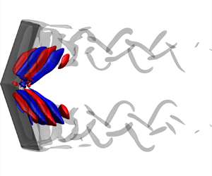
Figure 3. (a) Resolvent gains and (b) forcing–response mode pairs for $(sAR,\alpha,\varLambda ) = (4,20^\circ,0^\circ )$. For each mode, forcing ($\hat {\boldsymbol {f}}$) is the top half while response ($\hat {\boldsymbol {q}}$) it the bottom half with isosurfaces of velocity $\hat {u}_y \in [-0.2,0.2]$, with free stream directed to the right. Bottom panel of (a) shows power spectrum density of lift coefficient $\hat {C}_L$.

The spatial structures of forcing–response mode pairs are shown in figure 3(b) for representative frequencies. For $St = 0.14$, primary modes exhibit modal structures near the root plane. The forcing mode appears near and upstream of the wing, while the response mode develops downstream in the wake. The modal structures for the primary forcing and response modes are aligned with the wingspan, with the response mode similar to the unsteady vortices revealed from DNS. At this frequency, the secondary modes are comprised of spanwise-aligned vortices near the root plane, similar to the primary modes.

As we increase the frequency, the resolvent gains decay in magnitude and $\sigma _1$ decays faster than $\sigma _2$. Their magnitudes become approximately the same at $St = 0.16$. At this frequency, the spatial characteristics of the primary and secondary forcing–response mode pairs exhibit distinct behaviour. The primary forcing and response modes are aligned with the wingspan and near the root plane, similar to those at lower $St$. The secondary modes, however, exhibit modal structures near the wing tip, in contrast to the secondary modes at lower frequencies which reside near the wing root.

For $St = 0.18$, the primary forcing–response mode pair appears near the wing tip, while the secondary mode pair develops at the root plane. Such behaviour persists as we increase the frequency to $St = 0.20$. For $St \ge 0.18$, primary modes are tip-dominated while secondary modes are root-dominated around this wing. This means that root and wing tip modes switch their order of amplification at $St \approx 0.18$, i.e. mode switching.

The mode switching phenomenon is also observed for swept wings with $\varLambda = 15^\circ$. For such wings, root-supported structures appear as the primary forcing–response pairs at $St = 0.14$, as shown in figure 4(a). A distinct mode switching is observed over this wing, as the forcing–response pairs gradually transition towards the root at $z/c \approx 0$ with an increase in $St$. This type of concentrated resolvent mode at the wing root also appears for the unswept wings at $St = 0.20$ as a secondary mode, as shown at the bottom of figure 3(b).

Figure 4. Resolvent gain distribution for the top three mode pairs and forcing–response mode pairs for selected frequencies for $(sAR,\alpha ) = (4,20^\circ )$ and $\varLambda =$ (a) $15^\circ$, (b) $30^\circ$ and (c) $45^\circ$. Primary forcing ($\hat {f}$) and response ($\hat {q}$) modes shown with isosurfaces of velocity $\hat {u}_y \in [-0.2,0.2]$.

For $\varLambda = 30^\circ$, mode switching also occurs towards the root with an increase in $St$, in an opposite trend to that of the unswept wings. The dominant response modes at lower frequencies appear at the wing tip, as shown in figure 4(b). There is a gradual transition to root-supported modes as the frequency increases. At a higher sweep angle, $\varLambda = 45^\circ$, no mode switching occurs. The region of dominance of the forcing and response modes is slightly invariant for the frequencies shown herein.

In contrast with the lower-sweep-angle wings, for $\varLambda = 45^\circ$, forcing and response modes are dominant at distinct wingspan locations, as shown in figure 4(c). Response modes are tip-dominated while forcing structures appear upstream near the root plane, extending over the wingspan aligned with the sweep angle. For all $(sAR,\alpha ) = (4,20^\circ )$ wings, the highest amplification is found for $\varLambda = 30^\circ$, at $St \approx 0.12$. At $\varLambda = 45^\circ$, the dominant gain is an order of magnitude lower. This finding suggests that it is challenging to perturb flows over $\varLambda = 45^\circ$ wings. These wings are steady because self-sustained flow disturbances cannot introduce sufficient energy into the wake to generate vortex shedding.

3.2. Resolvent wavemakers

To characterize the self-sustained unsteadiness in the flows over swept wings, we study the spatial overlap between the forcing and response modes that supports the continuous formation of vortical structures. Since the forcing modes show regions receptive to external perturbations and the response modes reveal the structures being excited due to the forcing, the region over which forcing and response modes overlap can be interpreted as a mechanism for self-sustained oscillations in the flow. This idea is similar to the wavemaker concept deduced from direct and adjoint eigenmodes presented in Giannetti & Luchini (Reference Giannetti and Luchini2007).

Through the wavemaker analysis, previous studies identified critical points responsible for sustaining wake shedding on laminar wakes around cylinders (Strykowski & Sreenivasan Reference Strykowski and Sreenivasan1990; Hill Reference Hill1992) and regions associated with their primary and secondary instability modes (Giannetti & Luchini Reference Giannetti and Luchini2007; Giannetti et al. Reference Giannetti, Camarri and Luchini2010). Moreover, wavemakers revealed the physical mechanisms responsible for tonal noise generation in high-Reynolds-number flows over airfoils (Fosas de Pando, Schmid & Sipp Reference Fosas de Pando, Schmid and Sipp2017) and self-sustained flow instabilities in transonic buffet regimes (Paladini et al. Reference Paladini, Beneddine, Dandois, Sipp and Robinet2019).

In the aforementioned studies, wavemakers were derived from direct and adjoint global stability eigenmodes. Our formulation derives wavemakers from global resolvent modes and it is closely related to the structural sensitivity devised by Qadri & Schmid (Reference Qadri and Schmid2017) and to the resolvent wavemaker studied by Skene et al. (Reference Skene, Yeh, Schmid and Taira2022b). The present resolvent wavemaker is not identical to the eigenvector-based wavemaker. Using the time-averaged base flow, the present forcing terms encapsulate nonlinear effects as an internal feedback mechanism within the flow. Hence, the spatial overlap between forcing and response identifies regions responsible for self-sustained wake oscillations.

Herein, the resolvent wavemaker modes are directly obtained from the resolvent modes, as the Hadamard product of forcing and response modes:

(3.2)\begin{equation} \hat{\boldsymbol{w}} = \hat{\boldsymbol{f}} \circ \hat{\boldsymbol{q}}, \end{equation}

where $\hat {\boldsymbol {w}}$ is the resolvent wavemaker mode. The resolvent modes presented herein are defined with the five state variables, $\hat {\boldsymbol {f}} = [\hat {\boldsymbol {f}}_\rho,\hat {\boldsymbol {f}}_{u_x},\hat {\boldsymbol {f}}_{u_y},\hat {\boldsymbol {f}}_{u_z},\hat {\boldsymbol {f}}_T]$ and $\hat {\boldsymbol {q}} = [\hat {\boldsymbol {q}}_\rho,\hat {\boldsymbol {q}}_{u_x},\hat {\boldsymbol {q}}_{u_y},\hat {\boldsymbol {q}}_{u_z},\hat {\boldsymbol {q}}_T]$. We define our resolvent wavemaker gain $\xi$ as

(3.3)\begin{equation} \xi = \sigma^2 \int_{S} |\hat{\boldsymbol{w}}(\boldsymbol{x})|\,{\rm d}S, \end{equation}

which follows $\xi = \sigma ^2 | \langle \hat {\boldsymbol {f}},\hat {\boldsymbol {q}} \rangle |$, derived by Skene et al. (Reference Skene, Yeh, Schmid and Taira2022b). This is similar to that presented in Ribeiro et al. (Reference Ribeiro, Yeh, Zhang and Taira2022b). Qualitatively, both definitions of $\xi$ result in similar discussions and interpretations. The present expression for the resolvent wavemaker gain provides a proper quantitative definition (Skene et al. Reference Skene, Yeh, Schmid and Taira2022b). The resolvent wavemaker gain $\xi$ can also be computed for each spanwise slice and each frequency. To this end, we consider $S = S(x,y)$, as $z$-normal planes at different spanwise locations, to build the $\xi$ contours shown in figure 5. Through this analysis, we highlight the spatial support of the resolvent wavemaker over the wingspan.

Figure 5. Wingspan location of primary resolvent wavemakers with isocontours of $\xi$ for $0.05 \le St \le 0.25$ for $(sAR,\alpha ) = (4,20^\circ )$ wings with (a–d) $0^\circ \le \varLambda \le 45^\circ$. Resolvent wavemaker modes at $St = 0.14$ are shown with isosurfaces of $\hat {u}_y / \| \hat {u}_y \|_\infty = \pm 0.1$ and instantaneous $Q=1$ are grey-coloured isosurfaces.

Let us focus our resolvent wavemaker analysis on the flow over the unswept wing with $(sAR,\alpha,\varLambda ) = (4,20^\circ,0^\circ )$, as shown in figure 5(a). At $St=0.14$, triglobal resolvent wavemakers with high $\xi$ appear between $2 \lesssim z/c \lesssim 3$ in the near wake. The resolvent wavemakers at this region support the formation of unsteady root vortices that propagate downstream in the wake. This resolvent wavemaker region is also characterized by the formation of braid-like structures that connect to the root shedding as vortex loops (Zhang et al. Reference Zhang, Hayostek, Amitay, Burstev, Theofilis and Taira2020a). Resolvent wavemakers for $(sAR,\alpha,\varLambda ) = (4,20^\circ,15^\circ )$ also show similar shedding behaviour, as seen in figure 5(b).

Resolvent wavemakers are also revealed for steady flows. The overlap of forcing and response modes for flows over wings with $(sAR,\alpha,\varLambda ) = (4,20^\circ,30^\circ )$, as shown in figure 5(c), develops over the wing and extends into the wake aligned with the wing tip. These resolvent wavemakers extend over the entire wingspan, being stronger and larger than those exhibited around wings with lower sweep angles. The $\xi$ peak appears at the wing tip at $St = 0.12$, indicating that the tip region is more susceptible to develop unsteadiness around this wing.

For $\varLambda = 45^\circ$, shown in figure 5(d), we reveal that resolvent wavemakers emerge from the leading edge near the root plane towards the wing tip and downstream at the wake, overlapping the region where steady ram-horn-shaped vortices appear in the DNS. These resolvent wavemakers exhibit a region of the flow field with high receptiveness to amplify forcing structures and disturb the steady ram-horn vortex. Because the dominant resolvent wavemakers around the $\varLambda = 45^\circ$ wing have a low $\xi$, in spite of occupying a large region of the wake, the energy they introduce to the flow field is insufficient to disturb the wake.

The resolvent wavemakers further exhibit the root- and tip-dominated modal characteristics and the mode switching phenomenon in figure 5, in agreement with the forcing–response modal behaviour shown in figures 3 and 4. For instance, the resolvent wavemaker modes at the peak $\xi$ values for the unswept wing appear near $z/c \approx 2$, with a gradual transition from root-supported to tip-dominated modes as $St$ increases. Moreover, for the $\varLambda = 15^\circ$ wing, there is a transition in the dominant region of resolvent wavemaker support from $z/c \approx 1.5$ at lower frequencies to $z/c \approx 0$ at higher frequencies, as shown in figure 5(b). Lastly, for the $\varLambda = 30^\circ$ wing, there is a tip-to-root transition with an increase in $St$ while the peak resolvent wavemakers for $\varLambda = 45^\circ$ are invariant over the frequencies, appearing near $z/c \approx 2$.

3.3. Forcing-to-response dynamics

Let us further explain how perturbations emerge around swept wings, by analysing the overlap between the forcing and response modes in the spanwise direction. To this end, we integrate the norm of $\hat {\boldsymbol {f}}$ and $\hat {\boldsymbol {q}}$ over $z$-normal planes, analogous to the resolvent wavemaker mode analysis, as

(3.4a,b)\begin{equation} \boldsymbol{\varOmega}_{\hat{\boldsymbol{f}}}(z) = \int_{S(x,y)} \|\hat{\boldsymbol{f}}\|_2 \,{\rm d}S \quad \text{and} \quad \boldsymbol{\varOmega}_{\hat{\boldsymbol{q}}}(z) = \int_{S(x,y)} \|\hat{\boldsymbol{q}}\|_2 \,{\rm d} S, \end{equation}

where $\|\hat {\boldsymbol {f}}\|_2$ and $\|\hat {\boldsymbol {q}}\|_2$ are the $2$-norm of $[\hat {\boldsymbol {f}}_{\rho },\hat {\boldsymbol {f}}_{u_x},\hat {\boldsymbol {f}}_{u_y},\hat {\boldsymbol {f}}_{u_z},\hat {\boldsymbol {f}}_{T}]$ and $[\hat {\boldsymbol {q}}_{\rho },\hat {\boldsymbol {q}}_{u_x},\hat {\boldsymbol {q}}_{u_y},\hat {\boldsymbol {q}}_{u_z},\hat {\boldsymbol {q}}_{T}]$, respectively, at each grid point of the computational domain. By performing the integral over $S(x,y)$, we obtain $\boldsymbol {\varOmega }_{\hat {\boldsymbol {f}}}$ and $\boldsymbol {\varOmega }_{\hat {\boldsymbol {q}}}$ computed for each spanwise slice and for each frequency. Here, we plot their contours normalized by the maximum $\boldsymbol {\varOmega }_{\hat {\boldsymbol {f}}}$ and $\boldsymbol {\varOmega }_{\hat {\boldsymbol {q}}}$ at each $St$, to emphasize the spatial support of forcing and response over the wingspan, as shown in figure 6 for wings at $\alpha = 30^\circ$ with $0^\circ \le \varLambda \le 45^\circ$. The locations of the maximum strength of forcing and response modes are shown by the dot-dashed lines. Black arrows indicate the direction from the maximum forcing to the maximum response at $St = 0.15$. This analysis depicts the preferential direction in which optimal forcing is transferred to optimal response over the wingspan at each frequency.

Figure 6. Wingspan locations of dominant forcing (red) and response (blue) with contours of $\boldsymbol {\varOmega }_{\hat {\boldsymbol {f}}}$ and $\boldsymbol {\varOmega }_{\hat {\boldsymbol {q}}} \in [0.4,1.0]$ for $0.05 \le St \le 0.35$ for $sAR = 4$ wings with $\alpha = 30^\circ$ with (a–d) $0^\circ \le \varLambda \le 45^\circ$. Dot-dashed lines are polynomial fit of maximum $z/c$ of forcing and response at each $St$. Arrows show direction of optimal forcing to response at $St = 0.15$.

For unswept wings, shown in figure 6(a), the optimal forcing structures appear closer to the wing tip than the response modes, which are slightly shifted towards the root, suggesting that fluctuations are directed towards the root. Indeed, as seen in the DNS, unsteadiness is concentrated towards the root, as evident from figure 2, also in agreement with the results reported by Zhang et al. (Reference Zhang, Hayostek, Amitay, He, Theofilis and Taira2020b). In addition, the flow around the wing tip for unswept wings is characterized by an almost steady tip vortex, suggesting that it is likely hard to amplify flow oscillations near the tip.

For swept wings, fluctuations are directed towards the wing tip. For $\varLambda = 15^\circ$, both forcing and response modes appear near the wing root. At the vortex shedding frequency for this wing, $St \approx 0.15$, we observe forcing and response modes to be dominant at $z/c \approx 1$, with the forcing mode supported closer to the wing root than the response mode. This concurs with the flow field we observe in the DNS, as vortices are formed near the wing root and evolve towards the wing tip where spanwise vortices appear and propagate in the wake. For the $\varLambda = 30^\circ$ wing, the dominant forcing–response mode pair emerges near the wing tip at low $St$, as seen in figure 6(c). For this wing, low-frequency vortical structures emerge downstream in the wake aligned at the tip, as shown in figure 2.

For the $\varLambda = 45^\circ$ wing, the distance between the maximum forcing and response mode locations significantly increases. For this sweep angle, the region of forcing is centred at $z/c \approx 1$, while the response is supported mostly at $z/c \approx 3$. As the peak $\sigma _1$ is lower for this wing compared with lower-sweep-angle planforms, we argue that a significant amount of energy is required for an external forcing to perturb the wakes of highly swept wings. For all wings with $sAR=4$, this distance between the dominant forcing–response mode pairs is strongly associated with the sweep angle, while having a minor dependency on the angle of attack and presenting a gradual decrease with the frequency.

The direction from forcing to response revealed by the optimal triglobal resolvent modes suggests a spanwise advection of flow structures associated with the sweep angle. As shown previously, we can relate the forcing-to-response characteristics to the vortical fluctuations observed in the DNS. We can further relate these findings to the modal convective speed from biglobal stability analysis over swept wings (Crouch et al. Reference Crouch, Garbaruk and Strelets2019; Paladini et al. Reference Paladini, Beneddine, Dandois, Sipp and Robinet2019; Plante et al. Reference Plante, Dandois, Beneddine, Laurendeau and Sipp2021). Triglobal resolvent modes also reveal the advection of perturbations over the wingspan related to the sweep angle, the attenuation of flow unsteadiness and the resilience to amplify perturbations at high sweep angles. Even for unswept wings, the triglobal analysis uncovers a preferential root direction for advection of oscillations.

3.4. Influence of the aspect ratio

High sweep angle and low aspect ratio restrict the emergence of fluctuations in flows over finite wings. As shown in figure 6, tip- and root-dominated modes may extend over one or two chord lengths over the wingspan. For this reason, for flows over wings with $sAR < 2$, the dominance of the global modes may not be associated with root or tip regions, as they extend over the entire wingspan.

For flows over $sAR = 2$ wings, we observe a gradual transition between root-dominated and tip-dominated forcing and response modes, as shown in figure 7. For $\varLambda = 15^\circ$, the optimal forcing–response mode pair appears near the root for lower frequencies and at the wing tip for higher frequencies, characterizing a root-to-tip mode switching. For $\varLambda = 30^\circ$, the trend is opposite, with wing tip modes at lower frequencies and root modes at higher frequencies, characterizing a tip-to-root mode switching. These features are similar to the mode switching observed for these sweep angles with $sAR = 4$, as shown in figure 6.

Figure 7. (a–d) Wingspan locations of dominant forcing (red) and response (blue) with contours of $\boldsymbol {\varOmega }_{\hat {\boldsymbol {f}}}$ and $\boldsymbol {\varOmega }_{\hat {\boldsymbol {q}}} \in [0.4,1.0]$ for $0.05 \le St \le 0.35$ for wings at $\alpha = 30^\circ$, $sAR = 2$ and $1$ and $\varLambda = 15^\circ$ and $30^\circ$.

For wings with a low aspect ratio, the growth of root-dominated and tip-dominated perturbations is constrained and mode switching does not occur for $sAR = 1$, as shown in figure 8. Distinguishing between root-dominated and tip-dominated modes may be challenging for flows over $sAR = 1$ wings as forcing and response mode pairs appear globally, extending over the entire wingspan, independent of the sweep angle. Therefore, flows around wings with $sAR = 1$ tend to exhibit similar wake characteristics over different sweep angles. Indeed, the wake patterns for flows over $sAR = 1$ wings at a particular angle of attack and sweep exhibit characteristics different from those of the flows over higher-aspect-ratio wings, e.g. $sAR = 2$ and $4$.

Figure 8. Resolvent gain distribution and forcing–response mode pairs over frequency for $(\alpha,\varLambda ) = (30^\circ,15^\circ )$ and (a–c) $1 \le sAR \le 4$. Forcing ($\hat {f}$) and response ($\hat {q}$) modes shown with isosurfaces of velocity $\hat {u}_y \in [-0.2,0.2]$. Mode switching is absent for $sAR = 1$ due to merging of root and wing tip perturbations on the wake.

For high-aspect-ratio wings, for instance, the flow around $(sAR,\alpha,\varLambda ) = (4,30^\circ,15^\circ )$ wings, we observe in the DNS that the wake shedding structures appear over the entire wingspan. The resolvent modes depict these structures in three different flow mechanisms. As shown in figure 8(c) for $sAR = 4$, there are two types of root-dominated modes, which were also previously identified for this wing at $\alpha = 20^\circ$, shown in figure 4(a). The first one is characterized by root-dominated structures and appears at $St = 0.15$, while the second type, with a high $\sigma _1$, develops at $St = 0.25$ with compact root-concentrated modes. The third type is comprised of tip-dominated modes that become primary as the frequency increases to $St = 0.28$. These modes were primary at $\alpha = 20^\circ$ and $St \approx 0.40$, as shown in figure 4, although for $\alpha = 30^\circ$ they present a higher amplification gain.

For $sAR = 2$, root-dominated modes are primary for $St < 0.20$. Root-concentrated modes are absent and tip-dominated modes are the primary perturbations for $St \ge 0.20$, as shown in figure 8(b), characterizing a root-to-tip mode switching. The overall mode switching for $sAR = 2$ is the same, with root-to-tip transition. For $sAR = 1$, shown in figure 8(a), mode switching is absent. Both primary and secondary modes develop over the entire wingspan for all frequencies, as shown for the primary modes at $St = 0.14$. Although mode switching is absent we can still reveal two distinct root- and tip-dominated mechanisms on a single mode over low-aspect-ratio wings. For instance, at $St = 0.24$, modes emerge from the leading edge at the root and from the trailing edge near the tip. Combined, these two types of flow unsteadiness yield a global mode that appears over the entire wingspan.