


1. Introduction
Variable-density round jets arise in a wide number of industrial and environmental flows and represent therefore a widely investigated topic in fluid mechanics. For a complete and exhaustive review on early research works on these flows, the reader is referred to the book by Chen & Rodi (Reference Chen and Rodi1980), providing an overview of data collected in laboratory experiments and in the different flow regimes arising from such localized releases of varying density. According to a well-established classification (Chen & Rodi Reference Chen and Rodi1980), it is customary to identify three regions, characterized by different dynamical features: the near-field non-buoyant region, the far-field buoyancy dominated region and the intermediate region between the two, where buoyancy progressively counterbalances momentum. In the near field, the momentum flux overwhelms that of buoyancy. The resulting flow is therefore referred to as a ‘variable-density jet’, since any gravitational effect can be fully neglected, so that the momentum flux, evaluated over sections at increasing distance from the source, is kept constant (Panchapakesan & Lumley Reference Panchapakesan and Lumley1993; Hussein, Capp & George Reference Hussein, Capp and George1994). For increasing distances from the source and beyond a characteristic jet-length, denoted  $L_m$ (Morton Reference Morton1959), the role of gravitational effects begins to act on the flow dynamics, giving rise to a flow that is usually referred to as a ‘buoyant jet’ or a ‘forced plume’. Finally, for further larger distances from the source (typically exceeding $5L_m$), the momentum generation due to buoyancy becomes the main forcing of the flow, which then behaves as a ‘buoyant plume’ and whose dynamics do not differ from those of a plume induced by a source of pure buoyancy (Morton, Taylor & Turner Reference Morton, Taylor and Turner1956). It is worth noting that our interest here will be fully limited to the first (near-field) region, and we will therefore investigate effects induced by a variable density which are not due to its coupling with the gravitational field, i.e. which are independent from those usually referred to as buoyancy effects.
Results of early experimental works (Keagy Reference Keagy1949; Thring & Newby Reference Thring and Newby1953; Way & Libby Reference Way and Libby1971; Aihara, Koyama & Morishita Reference Aihara, Koyama and Morishita1974) have provided a first insight on key features of the dynamics of these flows and the appropriate scaling to recover self-similar analytical solutions for the velocity and density fields. Notably, this scaling was based on the definition of the ‘effective diameter’ when considering the momentum flux, by weighting the source diameter with the ratio between the (square root of the) density at the source  $\rho _s$ and that of the ambient fluid $\rho _0$. In subsequent experimental works, Panchapakesan & Lumley (Reference Panchapakesan and Lumley1993) and Kyle & Sreenivasan (Reference Kyle and Sreenivasan1993) succeeded in performing simultaneous measurements of fluid velocity and density (or temperature), therefore providing information on the cross-correlation statistics. Panchapakesan & Lumley (Reference Panchapakesan and Lumley1993) measured two velocity components and helium mass fraction concentration using a composite probe and an X-hot-wire anemometer. They focused on the intermediate region between the non-buoyant jet region and the plume region, provided accurate data on velocity and concentration statistics, and presented budgets for the turbulent kinetic energy and the scalar variance. Kyle & Sreenivasan (Reference Kyle and Sreenivasan1993) focused instead on the near field (up to a distance of less than ten source radii) using hot-wire anemometry, investigating the influence of the density ratio $\rho _s / \rho _0$ on the development of instabilities and triggering of breakdown in the jet dynamics.
Since the mid 1980s, experimental studies on variable-density jets have benefited from the development of optical measurement techniques. Using Rayleigh light scattering, Pitts (Reference Pitts1991a,Reference Pittsb) analysed the concentration field within variable-density jets, focusing on the role of density ratio and Reynolds number on the decay of time-averaged concentration and of its coefficient of variation, which he referred to as the ‘unmixedness’ value. Sautet & Stepowski (Reference Sautet and Stepowski1995), Amielh et al. (Reference Amielh, Djeridane, Anselmet and Fulachier1996) and Djeridane et al. (Reference Djeridane, Amielh, Anselmet and Fulachier1996) have reported detailed laser-Doppler anemometry (LDA) measurements of the turbulent velocity field in the near-field region of variable-density jets, providing valuable information on the structure of the transition region needed by the jet to attain self-similarity conditions, the Reynolds stress, the turbulent kinetic energy and higher-order velocity correlations. Combining LDA and cold wire, Pietri, Amielh & Anselmet (Reference Pietri, Amielh and Anselmet2000) and Darisse, Lemay & Benaïssa (Reference Darisse, Lemay and Benaïssa2013) obtained simultaneous measurements of two velocity components and temperature, which enabled them to estimate velocity and temperature correlations, turbulent fluxes, and hence turbulent viscosity and thermal diffusivity, yielding an estimate of the turbulent Prandtl number. More recently, Charonko & Prestridge (Reference Charonko and Prestridge2017) considered a vertical descending dense jet (air–SF $_6$ mixture), combining particle image velocimetry (PIV) and planar laser-induced fluorescence (PLIF), analysing variable-density effects on turbulent statistics and focusing on turbulent kinetic energy (t.k.e.) budgets. Viggiano et al. (Reference Viggiano, Dib, Ali, Mastin, Cal and Solovitz2018) studied instead the dynamics of light jets using PIV measurements. They focused on the effects of a varying Reynolds number on the jet dynamics and entrainment in the very near-field region (with a domain extent of four source diameters).
All these experimental results constitute a benchmark for the numerical simulations of variable-density jets performed with different approaches: Reynolds-averaged Navier–Stokes (Ruffin et al. Reference Ruffin, Schiestel, Anselmet, Amielh and Fulachier1994; Gharbi et al. Reference Gharbi, Ruffin, Anselmet and Schiestel1996), LES (Desjardins et al. Reference Desjardins, Blanquart, Balarac and Pitsch2008; Wang et al. Reference Wang, Fröhlich, Michelassi and Rodi2008; Foysi, Mellado & Sarkar Reference Foysi, Mellado and Sarkar2010) and direct numerical simulation (DNS) (Nichols, Schmid & Riley Reference Nichols, Schmid and Riley2007). An exhaustive comparison between numerical results and experimental data has been provided by Wang et al. (Reference Wang, Fröhlich, Michelassi and Rodi2008), who demonstrated the high accuracy of their LES results against the data set provided by the experiments of Djeridane et al. (Reference Djeridane, Amielh, Anselmet and Fulachier1996) and Amielh et al. (Reference Amielh, Djeridane, Anselmet and Fulachier1996).
Notwithstanding the relevant amount of studies on variable-density jets, there are still fundamental issues of their dynamics that require to be elucidated. On top of these is the influence of the local density ratio on the entrainment of ambient air within the jet. As shown by Kyle & Sreenivasan (Reference Kyle and Sreenivasan1993), a low density ratio (notably  $\rho _s / \rho _0 < 0.6$) has a large influence on the development of instabilities and oscillatory modes within the shear layers (for moderate Reynolds number at the source) in a free jet in its early stages of development. It is, however, unclear how this influence of the density ratio may persist in a fully turbulent jet and may influence the amount of ambient air entrained into the jet.
Therefore, the question that needs to be clarified is whether a jet that is lighter than the surrounding fluid entrains more than an iso-density jet or than a jet that is heavier than the surrounding fluid. The careful reader will certainly notice that the adjectives ‘light’ and ‘heavy’ are inappropriate here, since their meaning implies the relevance of the gravitational field, which we have discarded from the outset. According to the widespread jargon, we will however adopt this misuse of language, and refer to a momentum-dominated release which is less dense than the surrounding environmental fluid as a ‘light’ jet.
As far as we are aware, the first, and so far only, study providing insights on the dependence on the density ratio of the flux of ambient air entrained within variable-density releases is the seminal work of Ricou & Spalding (Reference Ricou and Spalding1961). By measuring the pressure difference across porous screens contouring vertical light and heavy momentum-dominated releases, they managed to estimate the variations of the mass flux, referred to here as  $G$, for increasing distances from the source. In scaling the evolution of $G$ with a corrected distance from the source, weighted by the square root of the ratio between the density at the source $\rho _s$ and that of the ambient fluid $\rho _0$, they implicitly proposed a model for the dependence of the entrainment rate on the jet density, predicting that the entrainment coefficient is reduced as the jet density becomes smaller. This finding is somehow striking, since it implies that the influence of a variable density via inertial effects on the entrainment rate would be opposite to that via buoyancy effects, which, as is well known, act in enhancing significantly the entrainment rate (Papantoniou & List Reference Papantoniou and List1989; Wang & Law Reference Wang and Law2002; Ezzamel, Salizzoni & Hunt Reference Ezzamel, Salizzoni and Hunt2015; van Reeuwijk et al. Reference van Reeuwijk, Salizzoni, Hunt and Craske2016).
In their study, Ricou & Spalding (Reference Ricou and Spalding1961) could rely only on global estimates of the jet mass flux which did not involve any velocity (nor density) measurement within the jet itself. This inevitably led to estimates of the mass flux growth averaged spatially, between the jet source and a characteristic distance  $z$, preventing near-field effects to be investigated. The near-field variations of the entrainment coefficient were instead investigated by Hill (Reference Hill1972), using an experimental apparatus similar to that used by Ricou & Spalding (Reference Ricou and Spalding1961), but allowing for estimates over shorter fetches. Hill (Reference Hill1972) reported the high variability of the entrainment coefficient close to the source (within 10 source diameters) in an air jet. Since then, a few other authors (Djeridane et al. Reference Djeridane, Amielh, Anselmet and Fulachier1996; Viggiano et al. Reference Viggiano, Dib, Ali, Mastin, Cal and Solovitz2018) have tackled the question of the effect of a varying density on the entrainment rate. Notably, Djeridane et al. (Reference Djeridane, Amielh, Anselmet and Fulachier1996) showed that the scaling proposed by Ricou & Spalding (Reference Ricou and Spalding1961) was not suited to model their experimental mass flux estimates in the near-field region. Lastly, based on PIV velocity measurements in helium jets, Viggiano et al. (Reference Viggiano, Dib, Ali, Mastin, Cal and Solovitz2018) estimated an entrainment coefficient in a field very close to the source (up to a distance of four source diameters). Similarly to Hill (Reference Hill1972), they reported the variation of the entrainment coefficient on the distance to the source and on the Reynolds number. According to their results, for a Reynolds number larger than 7000, both the entrainment coefficient and the normalized turbulent fluctuations become Reynolds-independent (the issue of the influence of the Reynolds number will be further discussed in § 3).
The lack of complete and detailed experimental studies of entrainment in variable-density jets is a direct consequence of the number of technical hurdles that must be faced when performing laboratory experiments with large differences in fluid densities. These are primarily due to the metrological difficulties of simultaneously measuring velocity and density fields in a turbulent flow with high density variations. In addition, increasing safety issues in several laboratories have limited the use of specific gases that are likely to be adopted for these experiments (e.g. hydrogen and SF $_6$).
The aim of our study is to contribute to fill this lack of knowledge and elucidate the mechanics of turbulent transfer and entrainment within a variable-density jet. Before presenting our methods, however, a caveat needs to be noted. Studying the effect of the variable-density ratio on the jet dynamics implies focusing on its near-field region (within few tens of source radii), where the density differences are actually relevant, but where the turbulent flow is also expected to be still affected by the release conditions. In principle, the effect of a varying density in the near field can be therefore hardly dissociated from those induced by varying conditions at the source, in terms of shape of the inlet velocity profile and of intensity of turbulent fluctuations (Boersma, Brethouwer & Nieuwstadt Reference Boersma, Brethouwer and Nieuwstadt1998), and those imposed at the boundary surrounding the source (see figure 1a,b). Considering this latter aspect, note that several studies in the turbulent jet literature, based on experiments (e.g. Hill Reference Hill1972; Ezzamel et al. Reference Ezzamel, Salizzoni and Hunt2015; Viggiano et al. Reference Viggiano, Dib, Ali, Mastin, Cal and Solovitz2018) and numerical simulations (e.g. van Reeuwijk et al. Reference van Reeuwijk, Salizzoni, Hunt and Craske2016), considered the case of releases issuing from a source placed within a rigid wall. A legitimate question then arises about the effects of this bottom wall (or similarly, of varying inlet velocity profiles) on the jet near-field dynamics and entrainment. Disentangling these effects from those induced by a variable-density ratio is therefore a crucial point.

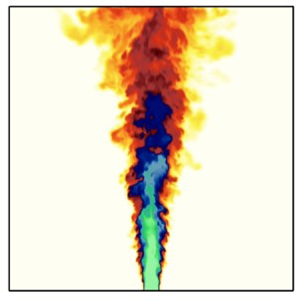
Figure 1. Schematic details of the boundary conditions at the source used for the numerical simulations (a) J1a–c (i.e. no bottom wall and pipe flow shaped inlet mean velocity profile) and (b) J3 (bottom wall and top-hat inlet mean velocity profile). Also shown for each case are the development of the jet and mean velocity profile for two distances from the source. (c) Instantaneous snapshot of the air-helium mixture mass fraction provided by the LES results (white,  $C=0$; green, $C=1$). (d) Image of the jet obtained by planar laser-induced fluorescence ( $22 \times 22$ mm $^2$ field of view).
To tackle this problem, we adopt an innovative approach combining experimental, numerical and theoretical methods for the investigation of the dynamics and the entrainment of freely propagating variable-density jets in a quiescent ambient fluid. The theoretical analysis, presented in § 2, relies on the so-called entrainment decomposition (van Reeuwijk et al. Reference van Reeuwijk, Salizzoni, Hunt and Craske2016). This theoretical framework, originally proposed by Priestley & Ball (Reference Priestley and Ball1955), was adopted in recent works to analyse entrainment in iso-density jets and Boussinesq plumes (Kaminski, Tait & Carazzo Reference Kaminski, Tait and Carazzo2005; Ezzamel et al. Reference Ezzamel, Salizzoni and Hunt2015; van Reeuwijk & Craske Reference van Reeuwijk and Craske2015; Craske, Salizzoni & van Reeuwijk Reference Craske, Salizzoni and van Reeuwijk2017) and fountains (Milton-McGurk et al. Reference Milton-McGurk, Williamson, Armfield and Kirkpatrick2020, Reference Milton-McGurk, Williamson, Armfield, Kirkpatrick and Talluru2021). We extend it here to the case of large density differences, i.e. formulating the plume equations using Favre averages. This decomposition allows the entrainment coefficient to be linked to the kinetic energy budget of the jet via terms involving first- and second-order velocity and density statistics, which are here estimated by means of experiments and numerical simulations.
Two density ratios at the source are investigated: a mixture of helium and acetone gas with  $\rho _s/\rho _0 \approx 0.4$ and an iso-density air jet. Experiments combining simultaneous PIV and LIF measurements provide both Reynolds and Favre averages of first- and second-order velocity and concentration statistics. Large eddy simulations of these flows were then performed (§ 3.2) to: (i) provide an accurate analysis of their reliability, taking advantage of the new complete experimental data set provided by the experiments; (ii) obtain further information on flow statistics that are hardly evaluated experimentally (other than pressure, these include also spatial derivatives of second-order statistics that are likely to be noisy when evaluated from experimental data); (iii) evaluate the effects on flow field and entrainment due to varying shape of the inlet mean velocity profile and the presence of a bottom wall surrounding the source. The profiles of experimental and numerical velocity and concentration statistics are presented in § 4, while azimuthally and radially averaged flow variables, i.e. those usually adopted in integral jet models, and entrainment coefficient are discussed in § 5.1. The results for the entrainment coefficient decomposition and the comparison between the low-density jet and the iso-density air jet are shown in § 5.2. Conclusions are drawn in § 6.
2. Theoretical aspects
We consider a release of a light fluid, having density  $\rho _s$, kinematic viscosity $\nu$ and molecular diffusivity $D$, issuing with a (spatially averaged) velocity $w_s$ from a circular source of radius $r_s$ and emitted within a still ambient fluid, whose density is referred to as $\rho _0$ (figure 1a,b). In a general way (we limit our interest to low-Mach-number flows), the dynamics of the variable-density jet is governed by four non-dimensional parameters. These are the Reynolds number ${Re_s = {w_s 2 r_s}/{\nu }}$, the Schmidt number ${Sc = {\nu }/{D}}$, the density ratio ${{\rho _s}/{\rho _0}}$, and a parameter quantifying the relative importance of inertial and buoyancy effects. In the research community dealing with variable-density jets, this latter parameter is usually expressed via the Froude number ${Fr_s = {\rho _s w_s^2}/{|\rho _s - \rho _0 | g 2 r_s }}$ (e.g. Chen & Rodi Reference Chen and Rodi1980; Djeridane et al. Reference Djeridane, Amielh, Anselmet and Fulachier1996). Among researchers more interested in buoyant (pure or forced) plumes, this is instead expressed using the Richardson number $Ri_s$. Based on the definition proposed by van Reeuwijk et al. (Reference van Reeuwijk, Salizzoni, Hunt and Craske2016), and adopted hereafter, the latter is defined as $Ri_s=({\rho _s}/{2 \rho _0})({1}/{Fr_s})$.
Our focus here is on fully turbulent flows (i.e.  $Re_s \rightarrow \infty$), whose first-order statistics are unaffected by molecular diffusion. In the framework of our analysis, the influence of the Schmidt number can therefore be discarded. Given these hypotheses, to retrieve jet integral equations (Morton et al. Reference Morton, Taylor and Turner1956), we model the flow using a low-Mach-number formulation of the Favre-averaged Navier–Stokes equations of an inviscid flow. The Favre averages are denoted by a tilde and defined as $\tilde {\xi }=\overline { \rho \xi }/ \bar {\rho }$ (so that the variance writes $\tilde {\sigma }^2_{\xi }=\overline {\rho (\tilde {\xi }-{\xi })^2 }/ \bar {\rho }$), where overbar denotes Reynolds average. Fluctuations from the Reynolds and Favre averages are then noted as $\xi '$ and $\xi ''$, respectively. We adopt a cylindrical system of coordinates $z$,
$z$,  $r$ and $\theta$ whose origin is placed at the centre of the circular source of the jet (see figure 1). Neglecting the role of viscosity and assuming a (statistically) axisymmetric and steady flow, the Favre-averaged conservation equations for mass and momentum (in the $z$-direction) can be expressed respectively as
 \begin{gather} \frac{1}{r}\frac{\partial}{\partial r} r (\bar{\rho}\tilde{u}) + \frac{\partial}{\partial z} (\bar{\rho}\tilde{w}) =0, \end{gather}
 \begin{gather}\frac{1}{r}\frac{\partial}{\partial r} r (\bar{\rho}\tilde{u}\tilde{w}+\bar{\rho}\widetilde{u''w''})+\frac{\partial}{\partial z} (\bar{\rho}\tilde{w}^{2}+ \bar{\rho}\widetilde{w''^{2}})={-}\frac{\partial}{\partial z} \bar{p} + \rho_0 \bar{b}, \end{gather}
where  $\bar {p}$ is the pressure difference relative to the hydrostatic pressure $p_0$ (defined such that $({\partial }/{\partial z}){p_0}=-\rho _0 g$, with $g$ the gravitational acceleration and where $\bar {b} = g (\rho _0 - \bar {\rho }) / \rho _0$ is the local buoyancy (Woods Reference Woods1997). Multiplying (2.2) by $2 \tilde {w}$ and using (2.1) yields
 \begin{align} &\frac{1}{r}\frac{\partial}{\partial r} r ( \bar{\rho}\tilde{u} \tilde{w}^{2} + 2 \bar{\rho}\widetilde{u''w''}\tilde{w} ) +\frac{\partial}{\partial z} (\bar{\rho}\tilde{w}^{3}+2\bar{\rho}\widetilde{w''^{2}}\tilde{w} +2\bar{p}\,\tilde{w})\nonumber\\ &\quad =2\bar{\rho}\widetilde{u''w''}\frac{\partial}{\partial r}\tilde{w}+2 \bar{\rho}\widetilde{w''^{2}}\frac{\partial}{\partial z}\tilde{w} +2\bar{p}\frac{\partial}{\partial z}\tilde{w} + 2 \rho_0 \bar{b} \tilde{w} . \end{align}
Integrating (2.1), (2.2) and (2.3) over  $r$ (between the jet axis and infinity), we then obtain
 \begin{gather} \frac{\mathrm{d}G}{\mathrm{d}z} ={-}2 \rho_0 [r \tilde{u}]_\infty, \end{gather}
 \begin{gather}\frac{\mathrm{d}}{\mathrm{d}z} (\beta_{g} M ) = \rho_0 B, \end{gather}
 \begin{gather}\frac{\mathrm{d}}{\mathrm{d}z} \left(\gamma_{g}\frac{M^2}{G} \right) = \delta_{g}\frac{M^{5/2}}{Q^{1/2} G^{3/2}} + \theta_m \frac{ B M }{G} , \end{gather}
where the mass flux,  $G$, momentum flux, $M$, volume flux, $Q$, and integral buoyancy, $B$, are defined respectively as
 \begin{align} G
\equiv 2\int_{0}^{\infty}\bar{\rho}\tilde{w}r\,\mathrm{d}
r,\quad M \equiv
2\int_{0}^{\infty}\bar{\rho}\tilde{w}^{2}r\,\mathrm{d}
r,\quad Q \equiv 2\int_{0}^{\infty}\tilde{w}r\,\mathrm{d}
r,\quad B \equiv 2 \int_{0}^{\infty} \bar{b} r \,\mathrm{d}
r,
\end{align}
\begin{align} G
\equiv 2\int_{0}^{\infty}\bar{\rho}\tilde{w}r\,\mathrm{d}
r,\quad M \equiv
2\int_{0}^{\infty}\bar{\rho}\tilde{w}^{2}r\,\mathrm{d}
r,\quad Q \equiv 2\int_{0}^{\infty}\tilde{w}r\,\mathrm{d}
r,\quad B \equiv 2 \int_{0}^{\infty} \bar{b} r \,\mathrm{d}
r,
\end{align}
and where  $\beta _g = \beta _m+\beta _f+\beta _p$, $\gamma _g = \gamma _m + \gamma _f + \gamma _p$ and $\delta _g = \delta _m + \delta _f + \delta _p$ are profile coefficients associated with the radial variations of the mean flow (denoted with subscript ‘ $m$’), velocity fluctuations (denoted with subscript ‘ $f$’) or with the mean pressure (denoted with subscript ‘ $p$’). The profile coefficients associated with the radial variations of the mean flow are defined as
 \begin{equation}
\left.\begin{array}{c} \displaystyle \beta_m \equiv
\dfrac{2}{\rho_m w_m^2 r_m^2} \int_0^\infty \bar{\rho}
\tilde{w}^2 r\, {\textrm d} r = 1,\quad \theta_m \equiv
\dfrac{2}{b_m w_m r_m^2} \int_0^\infty \bar{b} \tilde{w}
r\, {\textrm d} r,\\
\displaystyle \gamma_m \equiv
\dfrac{2}{\rho_m w_m^3 r_m^2} \int_0^\infty
\bar{\rho}\tilde{w}^3 r\, {\textrm d} r,\quad \delta_m
\equiv \dfrac{4}{\rho_m w_m^3 r_m} \int_0^\infty
\bar{\rho}\widetilde{w''u''}
\dfrac{\partial\bar{w}}{\partial r} r\, {\textrm d} r,
\end{array}\right\}
\end{equation}
\begin{equation}
\left.\begin{array}{c} \displaystyle \beta_m \equiv
\dfrac{2}{\rho_m w_m^2 r_m^2} \int_0^\infty \bar{\rho}
\tilde{w}^2 r\, {\textrm d} r = 1,\quad \theta_m \equiv
\dfrac{2}{b_m w_m r_m^2} \int_0^\infty \bar{b} \tilde{w}
r\, {\textrm d} r,\\
\displaystyle \gamma_m \equiv
\dfrac{2}{\rho_m w_m^3 r_m^2} \int_0^\infty
\bar{\rho}\tilde{w}^3 r\, {\textrm d} r,\quad \delta_m
\equiv \dfrac{4}{\rho_m w_m^3 r_m} \int_0^\infty
\bar{\rho}\widetilde{w''u''}
\dfrac{\partial\bar{w}}{\partial r} r\, {\textrm d} r,
\end{array}\right\}
\end{equation}and those associated with the fluctuations of the velocity or with the mean pressure are
 \begin{equation}
\left.\begin{array}{c} \displaystyle \beta_f \equiv
\dfrac{2}{\rho_m w_m^2 r_m^2} \int_0^\infty
\bar{\rho}\widetilde{w''^2} r\, {\textrm d} r,\quad
\beta_p \equiv \dfrac{2}{\rho_m w_m^2 r_m^2} \int_0^\infty
\bar{p} r\, {\textrm d} r, \\
\displaystyle \gamma_f\equiv \dfrac{4}{\rho_m w_m^3 r_m^2} \int_0^\infty
\bar{\rho} \tilde{w} \widetilde{w''^2} r\, {\textrm d}
r, \quad \gamma_p \equiv \dfrac{4}{\rho_m w_m^3 r_m^2}
\int_0^\infty \tilde{w} \bar{p} r\, {\textrm d} r, \\
\displaystyle \delta_f \equiv \dfrac{4}{\rho_m w_m^3 r_m}
\int_0^\infty \bar{\rho}\widetilde{w''^2}
\dfrac{\partial\bar{w}}{\partial z} r\, {\textrm d} r,
\quad \delta_p \equiv \dfrac{4}{\rho_m w_m^3 r_m}
\int_0^\infty \bar{p} \dfrac{\partial\tilde{w}}{\partial z}
r\, {\textrm d} r. \end{array}\right\}
\end{equation}
\begin{equation}
\left.\begin{array}{c} \displaystyle \beta_f \equiv
\dfrac{2}{\rho_m w_m^2 r_m^2} \int_0^\infty
\bar{\rho}\widetilde{w''^2} r\, {\textrm d} r,\quad
\beta_p \equiv \dfrac{2}{\rho_m w_m^2 r_m^2} \int_0^\infty
\bar{p} r\, {\textrm d} r, \\
\displaystyle \gamma_f\equiv \dfrac{4}{\rho_m w_m^3 r_m^2} \int_0^\infty
\bar{\rho} \tilde{w} \widetilde{w''^2} r\, {\textrm d}
r, \quad \gamma_p \equiv \dfrac{4}{\rho_m w_m^3 r_m^2}
\int_0^\infty \tilde{w} \bar{p} r\, {\textrm d} r, \\
\displaystyle \delta_f \equiv \dfrac{4}{\rho_m w_m^3 r_m}
\int_0^\infty \bar{\rho}\widetilde{w''^2}
\dfrac{\partial\bar{w}}{\partial z} r\, {\textrm d} r,
\quad \delta_p \equiv \dfrac{4}{\rho_m w_m^3 r_m}
\int_0^\infty \bar{p} \dfrac{\partial\tilde{w}}{\partial z}
r\, {\textrm d} r. \end{array}\right\}
\end{equation}
In these definitions, we have made use of a ‘top-hat’ jet width  $r_m$, velocity $w_m$, density $\rho _m$ and buoyancy $b_m$, which are consistently defined using integral quantities as (van Reeuwijk & Craske Reference van Reeuwijk and Craske2015)
 \begin{equation} r_{m} \equiv \frac{Q^{1/2}G^{1/2}}{{M^{1/2}}},\quad w_{m} \equiv \frac{M}{G},\quad \rho_m \equiv \frac{G}{Q}, \quad b_m \equiv \frac{BM}{QG}.\end{equation}
By definition of the entrainment coefficient, the radial volume flux of the entrained ambient fluid in (2.4) is assumed to be proportional to the longitudinal velocity of the jet:
 \begin{equation} \alpha \equiv \frac{- [r \tilde{u}]_\infty}{r_{m} w_m}.\end{equation}
Combining (2.4), (2.10a–d) and (2.11), the entrainment coefficient can be expressed as
 \begin{equation} \alpha = \frac{\rho_m}{\rho_0} \frac{r_m}{2 {G}} \frac{\mathrm{d}G}{\mathrm{d}z} . \end{equation}
Equations (2.5) and (2.6) in turn become
 \begin{gather} \frac{r_m}{M} \frac{\mathrm{d}}{\mathrm{d}z} (\beta_{g}M ) = Ri, \end{gather}
 \begin{gather}r_m \frac{G}{{M}^{2}} \frac{\mathrm{d}}{\mathrm{d}z} \left( \gamma_{g}\frac{{M}^{2}}{G} \right) = \delta_{g} + 2\theta_m Ri, \end{gather}
where  $Ri$ is the plume Richardson number, a parameter varying with the distance from the source, defined as
 \begin{equation} Ri \equiv \frac{b_m r_m}{w_m^2} = \frac{B}{M} \left ( \frac{QG}{M} \right )^{1/2}, \end{equation}
so that  $Ri(z=0)=Ri_s$.
Finally, by re-arranging (2.13) and (2.14), we can retrieve an alternative formulation of the entrainment coefficient:
 \begin{equation} \alpha_E = \underbrace{- \frac{\rho_m}{\rho_0} \frac{{\delta}_g}{2{\gamma}_g}}_{\alpha_{prod}} + \underbrace{\frac{\rho_m}{\rho_0} r_m \frac{{\textrm d} }{{\textrm d} z} \left( \ln \frac{{\gamma}_g^{1/2}}{\beta_g} \right) }_{\alpha_{shape}} + \underbrace{\frac{\rho_m}{\rho_0} \left(\frac{1}{\beta_g}-\frac{\theta_m}{\gamma_g}\right) {Ri} } _{\alpha_{Ri}}.\end{equation}
The first term on the right-hand side of (2.16), referred to as  $\alpha _{prod}$, represents the contribution to the entrainment directly linked to the turbulent kinetic energy production. The second term, referred to as $\alpha _{shape}$, depends instead on the change in shape of the mean velocity and Reynolds stress radial profiles. The third term, $\alpha _{Ri}$, is related to buoyancy effects, and, as we will show next, is fully negligible in the variable-density jet considered here.
The scope of the present work is to unveil the influence of a variable density on the three terms composing (2.16). Density variations will of course act directly through the density ratio  $\rho _m / \rho _0$ (and eventually the Richardson number), but they will also act indirectly by changing the values of the profile coefficients, i.e. $\delta _g$, $\gamma _g$ and $\theta _m$. Therefore, our aim here is to: (i) estimate the value of the coefficients (2.8) and (2.9) by means of experiments and LES; (ii) analyse the relative role of the three terms composing the entrainment relation (2.16), with a focus on $\alpha _{prod}$ and $\alpha _{shape}$; (iii) analyse how these are influenced by varying boundary conditions (inlet velocity profile and presence of a bottom wall); and (iv) discuss the evolution of the profile coefficients and of the entrainment rate with respect to data collected in iso-density jets.
3. Experimental and numerical methods
The analysis of the statistics of the velocity and density fields relies on two data sets. One is obtained by performing laboratory experiments (§ 3.1) and the other by performing LES (§ 3.2). As an illustration of the flow development, visualizations of the jet obtained by means of LES and experiments are presented in figures 1(c) and 1(d), respectively.
3.1. Laboratory experiments
Velocity and concentration measurements were performed using two jets of different densities expanding in air at rest and at ambient temperature and pressure (Moutte Reference Moutte2018). Two jets are produced. One, referred to as ‘light’ and having a density ratio  $\rho _s/\rho _0 = 0.39$, is produced by the release of a mixture of helium and acetone vapour. The second, referred to as ‘iso-density jet’ and having $\rho _s/\rho _0 = 1.17$, is produced by a mixture of air and acetone vapour. Glass atomizers (perfume diffusers) provide a micronic olive oil aerosol as seeding for PIV. As the amount of oil injected is small, it does not change the density of each release. Note that both jet and ambient air are seeded to avoid any bias in velocity measurements. For each experiment, the source release parameters are given in table 1. The experimental set-up is shown in figure 2 and its main characteristics are outlined below.
Table 1. Experimental conditions. The main results concern the light jet (figures 3–5 and 6–11) and they are compared to air jet results in figure 11.


Figure 2. Sketch of the experimental set-up (Moutte Reference Moutte2018). The main elements are as follows: (0) camera for PIV, (1)  $200$ mm lens, (2) pulsed laser, (3) camera for PLIF, (4) $532$ nm optical filter, (5) light intensifier, (6) dichroic mirror, (7) optical table, (8) containment box, and (9) jet maker.
The pipe jet nozzle has a radius  $r_s = 1.75$ mm and its edge thickness is $0.35$ mm. The ratio between the length of the pipe $l$ and the ejection radius is equal to $l/r_s = 80$ that insures the development of a fully turbulent pipe flow as inflow conditions of the jet. The jet spans in a square Plexiglas enclosure of $L = 300$ mm side, so that the section ratio $L^2/({\rm \pi} r_s^2) >9000$ is large enough to avoid confinement effects. The values of $Re_s$ and $Fr_s$ (see table 1) are the same as those of the experiments by Djeridane et al. (Reference Djeridane, Amielh, Anselmet and Fulachier1996) and Amielh et al. (Reference Amielh, Djeridane, Anselmet and Fulachier1996). Note that what we refer to as ‘iso-density’ jet is indeed a slightly dense jet (due to the presence of acetone as a tracer) having $Fr_s=571\ 000$ and $Re_s=16\ 400$, a value at which the entrainment process can be considered as Reynolds independent, according to the analysis presented by Ricou & Spalding (Reference Ricou and Spalding1961). For the light release, we have instead $Fr_s=120\ 000$, a value sufficiently high to discard any influence of buoyancy effects, and $Re_s= 7000$. Consider however that data of Pitts (Reference Pitts1991b) on dense jets suggest that, for $Re_s > 7000$, the average and the variance of the concentration do not show any relevant effect due to the variation of the Reynolds number. These findings have been recently confirmed by Viggiano et al. (Reference Viggiano, Dib, Ali, Mastin, Cal and Solovitz2018), who concluded, based on PIV measurements in helium jets, that, as $Re_s > 7000$, both the entrainment coefficient and second-order flow statistics become Reynolds independent.
The optical arrangement allows for the measurements of the two-dimensional velocity field by PIV and of the mass fraction field by PLIF, both fields being simultaneously measured in time and space (see figure 2). A single, dual cavity pulsed Nd:YAG laser (2) provides illumination with both frequency-doubled 532 nm (Quantel Big sky Laser, visible, at 170 mJ per pulse) and frequency-quadrupled 266 nm (UV, at 31 mJ per pulse) outputs. The illumination is synchronized by two timer boxes (National Instruments NI-PCI 6602) with the image acquisition on two sensitive CCD cameras. The visible and UV laser beams (7) are conditioned by successive dichroic mirrors and lenses to generate two overlying laser beams expanded into a single sheet by a cylindrical lens that illuminates the same flow plane in a  $22 \times 22\ \textrm {mm}^2$ field of view. The PIV images are acquired by a Hamamatsu Hisense 4M camera (12 bpp, $2048 \times 2048$ pixels, 5 Hz) (0) fitted with a 200 mm lens (1) at $f$/22 aperture equipped with a pass-band optical filter centred at 532 nm. The fluorescence of the acetone vapour carried within the mixture is stimulated by the 266 nm wavelength of the laser. PLIF images (figure 1d) are obtained with a very sensitive, cooled, Hamamatsu Hisense 4M camera (12 bpp, $2048 \times 2048$ pixels, 5 Hz) (3) coupled to a high-speed gated Hamamatsu intensifier (Photocathode GaAsP type P46) (5) to increase the low fluorescence signal collected in the 350–550 nm range. A low-pass filter is placed on the PLIF path to cut wavelengths above 532 nm. This filter is placed in front of the 200 mm lens at the $f$/4 aperture (4). The observation of the same field of view is insured by a dual camera mount (6) (Dantec Dynamics) consisting in a dichroic mirror that reflects light towards the PIV camera (0) and transmits light to the PLIF camera (3). To each pair of PIV images acquired with an adjusted delay of a few $\mathrm {\mu }$s is associated one PLIF image synchronously acquired with the second PIV image. A total of 4000 triplets of images documenting the velocity field and the concentration field are therefore acquired at a rate of 5 Hz, at the same location in the same plane. The whole system is controlled by the Dynamic Studio Software (DANTEC Dynamics). The correlation of PIV images is performed by the adaptative PIV algorithm with $32 \times 32$ pixel boxes, with 50 % overlap. The spatial resolution of the PIV measurements was $16\ \textrm {pixels} / 2048\ \textrm {pixels} \times 22\ \textrm {mm} = 0.17\ \textrm {mm}$. To obtain the same resolution for the LIF, which was initially resolved to the scale of one pixel, a binning of the data over 16 pixels was applied.
Successive steps are considered to obtain the concentration field from raw PLIF images. The shot-by-shot laser intensity variation was estimated through the standard deviation of the spatial mean of the raw grey levels for the 4000 PLIF images, giving 1.9 % on the whole image surface and 1.2 % in the potential core at the jet exit. These standard deviations include also the fluctuations of the saturated pressure of acetone vapour in helium that is obtained by bullying a helium flow part in a liquid acetone tank maintained at  $24.2\,^\circ \textrm {C} \pm 0.5\,^\circ \textrm {C}$ in an open heating bath circulator. The background noise level $G_{noise}$ is estimated with the space–time averaging of one hundred images of the field of view acquired with the laser light but without any flow, then $G_{noise}$ is subtracted from the grey level $G(x,y,t)_{raw}$ of each raw PLIF image,
 \begin{equation} G(x,y,t)=({G(x,y,t)}_{raw}-G_{noise})/(L(x)). \end{equation}
The streamwise spatial inhomogeneity  $L(x)$ of the laser intensity profile was determined by illuminating with the UV laser sheet a quartz tank filled by the helium jet marked by acetone vapour. For this procedure, the averaged image over one hundred acquired images is used. A final adjustment of $L(x)$ is made by checking the conservation of mean acetone quantity obtained for each section during measurements (Sarathi et al. Reference Sarathi, Gurka, Kopp and Sullivan2011; Charonko & Prestridge Reference Charonko and Prestridge2017). Since the optical density ( $OD=57$ mm) is estimated to be one order of magnitude greater than the radial expansion of the more dense region of the jet ( $D_j=3.5$ mm) for a 13.9 % molar fraction of acetone vapour in helium, the Beer law was not considered for any laser beam attenuation correction (Lozano, Yip & Hanson Reference Lozano, Yip and Hanson1992). The induced error measurement is estimated to 2 % on the jet axis concentration value in the very near region of the jet development. The grey level $G(x,y,t)$ is then related to molar fraction $\chi$ by a linear transformation, imposing $\chi =1$ in the jet potential core and $\chi =0$ in the ambient air, outside the jet. The mass concentration $C$ is finally deduced from $\chi$ as $C={\chi \rho _s/\rho _0}/({1-\chi (1-\rho _s/\rho _0)})$. Velocity, mass fraction and their coupling statistical moments are calculated with home-made MATLAB programs. Eight fields of view are successively investigated to describe the jet development, longitudinally and radially, from its exhaust up to 64 $r_s$.
Following Sciacchitano & Wieneke (Reference Sciacchitano and Wieneke2016) and Milton-McGurk et al. (Reference Milton-McGurk, Williamson, Armfield and Kirkpatrick2020), we consider that, at first-order, the most relevant source of the experimental errors is due to precision uncertainty, due to the finite number of samples. They have been estimated here according to the procedure presented by Benedict & Gould (Reference Benedict and Gould1996), which we have applied focusing on three distances from the source ( $z/ r_s= 2, 16, 36$) and two radial positions (jet centre and jet half-width), considering a 95 % confidence interval. Concerning the mean longitudinal velocities, the experimental error is of the order of 1 %, except in the very near field, where it accounts for approximately 3 % on the axis and attains 9 % on the jet half-width. The mean radial velocity is instead affected by significant errors (60 %) in the very near field that reduce to 30 % in the rest of the domain. The uncertainty on the mean and standard deviation of concentration is similar, with a maximal value that slightly exceeds 1 %, at the jet border in the far field. Uncertainty for the standard deviation of the velocity is generally between 2 % and 3 %. Finally, Reynolds stress is affected by an error of approximately 7 %, which is also representative for the velocity-concentration correlations in the far field. Errors for this latter variable are instead larger in the very near field and can almost attain 15 %.
3.2. Numerical simulations
The light (J1a–c, J2 and J3) and iso-density (J0) jets were numerically simulated using the code CALIF ${^3}$S (developed at the Institut de Radioprotection et de Sûreté Nucléaire – IRSN), solving a low-Mach-number formulation of Favre-filtered Navier–Stokes equations adopting a LES approach. In Cartesian coordinates, the mass, momentum and species transport equations are
 \begin{gather} \frac{\partial {\rho}}{\partial t}+\frac{\partial ({\rho}{u_i})}{ \partial{x_i}}=0, \end{gather}
 \begin{gather}\frac{\partial ({\rho}{u_i}) }{\partial t}+\frac{\partial ({\rho}{u_i}{u_j})}{\partial{x_j}}={-}\frac{\partial {p}}{\partial{x_i}}+\frac{\partial {S}_{ij}}{\partial{x_j}}- \frac{\partial \tau_{ij}}{\partial x_j} + \rho g_i, \end{gather}
 \begin{gather}\frac{\partial ({\rho}{C} )}{\partial t}+\frac{\partial ({\rho}{C} {u_i})}{\partial{x_i}}=\frac{\partial}{\partial{x_i}} \left ({\rho}D\frac{\partial {C}}{\partial{x_i}}+\frac{\mu_s}{Sc_s}\frac{\partial {C}}{\partial x_i} \right), \end{gather}
where  ${u_i}$ is the Favre-filtered velocity, ${p}$ is pressure, $g_i$ is the gravitational acceleration, ${C}$ is helium mass fraction, $D$ is the molecular diffusivity of the air–helium mixture, ${\mu _s}$ is the subgrid turbulent dynamic viscosity and $Sc_s$ is the subgrid turbulent Schmidt number. The density ${\rho }$ is the filtered density of the fluid computed as ${ {\rho } = ( {C}/{\rho _s} + ({1-C})/{\rho _0})^{-1 } }$. In (3.3), $\tau _{ij}$ represents the subgrid scale Reynolds stress, here evaluated by means of three different models: the Vreman model (Vreman Reference Vreman2004) for simulations J0, J1a, J2 and J3, the dynamical Smagorinsky model (Germano et al. Reference Germano, Piomelli, Moin and Cabot1991) for J1b and the WALE (wall adapting local eddy) model (Nicoud & Ducros Reference Nicoud and Ducros1999) for J1c. For the six simulations, the corresponding boundary conditions and subgrid model used are given in table 2. The term ${S}_{ij}=-(2/3)\mu (\partial {u_k}/\partial x_k)\delta _{ij}+\mu (\partial {u_i}/\partial x_j+\partial {u_j}/\partial x_i)$ is the filtered strain rate tensor, where $\mu$ is the molecular dynamic viscosity calculated as a function of the individual viscosities and molar masses as well as the corresponding mass fractions. In (3.4), the simple gradient diffusion hypothesis (SGDH) is used to close the problem with a turbulent subgrid Schmidt number $Sc_s$ set equal to $0.7$. We use a staggered grid with a cell-centred piece-wise constant representation of the scalar variables and a marker and cell (MAC) type finite-volume approximation for the velocity. For the time discretization, we employ a fractional step algorithm decoupling balance equations for the transport of species and Navier–Stokes equations which are solved by a pressure correction technique. Since we consider jets in an infinite (open) environment, the computational domain must be bounded by artificial boundary conditions which perturb as less as possible the flow in the interior of the domain. In our simulations, the imposed boundary conditions are based on the usual control of the kinetic energy and allow to distinguish between the flow that enters the domain and the flow that leaves it. This type of boundary condition was originally established for the incompressible case by Bruneau & Fabrie (Reference Bruneau and Fabrie1994, Reference Bruneau and Fabrie1996) and its extension to compressible flows was tackled by Bruneau (Reference Bruneau2000). The domain is a cube of size $40 r_s$. A refined Cartesian grid is used with a uniform square mesh ( ${\rm \Delta} x \times {\rm \Delta} y$) in the central part of the domain $\varOmega _1= [-5r_s: 5r_s]$, where the horizontal grid size is $r_s/14$. Outside $\varOmega _1$ and along the horizontal direction, the domain is divided into three successive subdomains, namely $\varOmega _2 = [-6r_s: -5r_s] \cup [5r_s: 6r_s]$, $\varOmega _3= [-10r_s: -6r_s] \cup [6r_s: 10r_s]$ and $\varOmega _4= [-20r_s: -10r_s] \cup [10r_s: 20r_s]$. The horizontal grid spacing is equal to $r_s/10$ over $\varOmega _2$ and $r_s/5$ over $\varOmega _3$. Over the last subdomain $\varOmega _4$, the grid is progressively stretched for increasing distance from the jet axis and the grid points are spread according to a geometric sequence of ratio 1.2 starting at a horizontal distance of $10r_s$ with an initial grid size of $r_s/3$.
Table 2. Boundary conditions, subgrid models and density ratio at the source adopted in the numerical simulations.

At the source, to trigger the transition to turbulence, the inlet flow has been perturbed with the method presented by Jarrin et al. (Reference Jarrin, Benhamadouche, Laurence and Prosser2006). The latter has been conceived to reproduce inflow conditions in wall-bounded flow (even characterized by complex geometries) with prescribed first- and second-order one point statistics, characteristic length and time scales. For the time discretization, a CFL (Courant–Friedrichs–Lewy) number close to unity has been imposed for each calculation even if time step sizes for which CFL numbers greater than one are allowed with the use of implicit schemes. Each simulation lasted  $1000 T$, where $T= r_s / w_s$ is a characteristic time scale. Results for the first $400 T$ were discarded and flow statistics were then computed over an interval of $600 T$. Mehaddi et al. (Reference Mehaddi, Vaux, Candelier and Vauquelin2015) and Vaux et al. (Reference Vaux, Mehaddi, Vauquelin and Candelier2019) compared results provided by the aforementioned LES approach of turbulent miscible Boussinesq and non-Boussinesq flows with experimental data, showing the reliability of the CALIF $^3$S code to properly reproduce the dynamics of turbulent buoyant flows characterized by large density differences.
To investigate the effect of varying source conditions (shape of inlet profile and presence of bottom wall) on the light jet dynamics, we have performed three numerical simulations using systematically Vreman as the subgrid model. The reference simulation, referred to hereafter as J1a (see figure 1a), represents a free jet (no bottom wall) with a typical pipe flow (a  $1/7$ power law) as the mean velocity profile at the nozzle, similar to that used in the experiments. For the second simulation (J2), the mean velocity profile at the source is uniform, usually called ‘top-hat’. In the third simulation, referred to as J3, we impose a top-hat inlet mean velocity profile and add a bottom wall surrounding the source (see figure 1b).
4. Local flow statistics
The starting point of our analysis is a detailed comparison between our experimental and numerical data. We will examine longitudinal profiles on the jet axis (§ 4.1) and radial profiles at different distances from the source (§ 4.2). Aims of this analysis are to evaluate: (i) the reliability of LES in reproducing the variable-density jet dynamics; (ii) the influence of varying source conditions (inlet velocity profile and presence of a bottom wall) on the flow statistics; (iii) the sensitivity of LES to varying the subgrid scale model. For brevity, in the following analysis, we only report data concerning the low-density release. In a general way, however, the considerations made hereafter (with respect to the three aforementioned aspects) apply equally to the iso-density case.
4.1. Longitudinal profiles on the jet axis
The comparison between experimental and LES data along the jet axis is presented in figure 3. The results show that the numerical results for the mean longitudinal velocity (figure 3a) are sensitive to the shape of the inlet profile. The results for the simulation reproducing the pipe flow follow accurately the trend of the experimental data, with a slight discrepancy at the farthest measurement station ( $z/r_s = 36$). The two simulations performed imposing a top-hat velocity profile show instead a clear trend in underestimating the centreline velocities (figure 3a). Despite these differences between the simulations, the profiles of the mean helium concentration, for the three cases considered, are very similar to each other and show very good agreement with the experimental data (figure 3b). Similarly, the estimates of the jet half-width, evaluated as the radial distance at which the centreline velocity and concentration are halved (and referred to as $r_w$ and $r_c$, respectively) are very well reproduced by the numerical simulations (both considering the mean velocity and concentration) regardless of the inlet profiles imposed at the source (figure 3c). The ratio between the two half-widths, usually referred to as $\phi$ (Wang & Law Reference Wang and Law2002; Ezzamel et al. Reference Ezzamel, Salizzoni and Hunt2015), is larger than unity and exceeds 1.3 far from the source. This is a common feature in iso-density jets, for which literature data indicate values in the range of $1.1 < \phi < 1.4$ (Craske et al. Reference Craske, Salizzoni and van Reeuwijk2017).

Figure 3. Decay of (a) the mean streamwise velocity and (b) the mean helium concentration along the jet axis. (c) Increase of the mean streamwise velocity half-width ( $r_w$) and the mean concentration half-width ( $r_C$). Axial evolution of the (d) longitudinal and (e) radial velocity fluctuations, and (f) of the concentration fluctuations. Black circles, experiments; black dotted lines, reference simulation (J1a); red dashed lines, simulation without bottom wall and top-hat profile for the inlet velocity (J2); blue dash–dotted lines, simulation with bottom wall and using top-hat profile for the inlet velocity (J3).
The three plots (figure 3d–f) presenting the longitudinal profile of the r.m.s. of the velocity (streamwise and radial components) and concentration provide a coherent picture. In the very near field ( $z/r_s < 10$), the numerical simulations (regardless of inlet profile and presence of the wall) reproduce accurately the rise of turbulent fluctuations. The numerical results tend subsequently to overestimate the experimental data, over a fetch of approximately ten source radii, over which the LES results attain more rapidly r.m.s. values characterizing the far field of iso-density jets, typically ${\widetilde {{\sigma _{w}}}} / \tilde {w}_c \simeq 0.26$ and ${\widetilde {{\sigma _{u}}}} / \tilde {w}_c \simeq 0.2$ (Wygnanski & Fiedler Reference Wygnanski and Fiedler1969; Hussein, Capp & George Reference Hussein, Capp and George1994). This higher rapidity observed in the rise of r.m.s. along the jet axis is likely to be due to the way in which inertial instabilities are triggered in the numerical simulations. Typically, these can be produced by forcing the inlet flow with an uncorrelated random noise (van Reeuwijk et al. Reference van Reeuwijk, Salizzoni, Hunt and Craske2016) or, as in this case, adopting more sophisticated algorithms (Jarrin et al. Reference Jarrin, Benhamadouche, Laurence and Prosser2006) in which velocity fluctuations are correlated one to the other, reproducing a synthetic turbulent velocity field characterized by typical length and time scales.
4.2. Radial profiles
To widen our understanding about the velocity and concentration fields we extend our analysis to the radial profiles of the flow (first- and second-order) statistics, which are here presented at three different distances from the source. First-order statistics are presented in figure 4, normalized with their respective centreline value. The near-field ( $z/r_s = 2$) streamwise velocity profiles are, as expected, influenced by the shape of the profile imposed at the source (figure 4a). The simulations with an inlet top-hat profile show clear discrepancies with the measured data, which are instead very well reproduced by imposing a pipe-flow profile. Placing the inlet on a rigid wall has very little influence on the core of the radial profile and affects only its tails. To appreciate this, we have also reported in figure 4(a) the profiles plotted with a logarithmic scale on the vertical axis. For the experimental case, we can observe then the presence of a light co-flow (induced by the jet) away from the source, accurately reproduced by the LES data (irrespective of the shape of the inlet profile imposed). This co-flow is instead suppressed when placing a rigid wall at the bottom boundary of the domain. For increasing distance from the source ( $z/r_s = 16$), the presence of the wall still induces slight differences between the shapes of the tails of the profiles (figure 4b). At the farthest distance, $z/r_s = 36$ (figure 4c), the results for the three simulations are almost identical and in good agreement with the experimental data. We will further discuss these features in § 5.2, when analysing how the inlet profile and bottom wall affect the profile coefficients (notably $\gamma _m$) and the entrainment rate. Shape variations of the inlet velocity profile and the presence of a bottom wall have instead no particular effect on the mass fraction field (figure 4d–f). The radial profiles of $\tilde {C}(r,z)$ are very similar for the three simulations and agree well with the experimental data, with only slight discrepancies on the jet borders in the far field. The mean radial velocity $\tilde {u}(r,z)$ is the variable that presents the main discrepancies between experimental and numerical estimates (figure 4g–i). This is not surprising, since, as discussed in § 3.1, the radial velocity is the variable that is affected (by far) by the largest precision uncertainty, attaining almost 60 %. Further note that bias error induced by slight uncertainties in the orientation of the measurement plane (even though specific attention was paid to the fact that both $\tilde {u}$ and $\widetilde {w''u''}$ must be equal to zero on the jet axis) may significantly affect the PIV estimate of the radial velocity. In any case, the discrepancies observed for $\tilde {u}(r,z)$ are much larger than those observed on the streamwise component. However, since these two variables, $\tilde {w}(r,z)$ and $\tilde {u}(r,z)$, are strictly linked together via the continuity equation, there is no grounded physical justification for these differences.

Figure 4. (a–c) Radial evolution of the mean streamwise velocity, (d–f) the mean concentration and (g–i) the mean radial velocity. The distance to the source of the jet is fixed to (a,d,g)  $z/r_s = 2$, (b,e,h) $z/r_s = 16$ and (c,f,i) $z/r_s = 36$. Same symbols and lines as in figure 3.
Second-order flow statistics, including velocity-concentration correlations, are presented in figure 5. In a general way, the numerical simulations reproduce well the shape of the experimental profiles. This is notably the case of the r.m.s. of the velocity fluctuations, whose intensity, however, is clearly overestimated by the numerical results (see figures 5b and 5e) in the intermediate field ( $z/r_s=16$). As already pointed out when commenting on the longitudinal profiles (presented in figure 3), this is due to a tendency of the numerical simulation to evolve more rapidly towards a fully turbulent flow within the core of the jet, due to the disturbances generated at the inlet by a synthetic eddy method (Jarrin et al. Reference Jarrin, Benhamadouche, Laurence and Prosser2006). Despite this, the profiles of the r.m.s. of the concentration are very well reproduced numerically (figure 5g–i). The only discrepancies can be observed at the farthest position where the experimental profile shows an anomalous peak at $r/r_s=5$, which is likely to be due to measurement errors (figure 5i).

Figure 5. Radial evolution of the (a–c) longitudinal and (d–f) radial velocity fluctuations, (g–i) concentration fluctuations, ( j–l) Reynolds stress, (m–o) radial velocity-concentration correlation and (p–r) turbulent Schmidt number. The distance to the source of the jet is fixed to (a,d,g,j,m,p)  $z/r_s = 2$, (b,e,h,k,n,q) $z/r_s = 16$ and (c,f,i,l,o,r) $z/r_s = 36$. Same symbols and lines as in figure 3.
The radial turbulent momentum transfer, as quantified by the normalized Reynolds stress profiles, is also simulated quite accurately (figure 5j–l) in terms of both the shape of the profiles and their peak value, with apparent discrepancies in the core of the jet in the near field (reasonably due to variation of the inlet conditions) and at the jet boundaries in the far field (for  $z/r_s = 36$). Concerning the radial turbulent mass transfer, the general picture is more critical. The radial turbulent mass flux (figure 5m–o) is undoubtedly the flow variable (among those considered here) characterized by the highest discrepancies between numerical and experimental estimates. These can be explained, at least partially, by the relevant (approximately 14 % in the near field) precision error on $\widetilde {C''u''}$ (§ 3.1). Note, however, that among the variables analysed here, $\widetilde {C''u''}$ is the most difficult to estimate experimentally, since it requires the coupling of two independent (but simultaneous) acquisitions. Therefore, even slight bias errors in the estimate of the velocity field, on one side, and on the concentration field, on the other, would boost then the overall experimental uncertainty in the estimate of $\widetilde {C''u''}$. Consider for example the profiles of $\widetilde {C''u''}$ in the very near field, i.e. $z/r_s=2$ (figure 5m), where the discrepancy between the two sets of data is significantly larger than that observed in the relative profiles of $\widetilde {\sigma _u}$ (figure 5d) and of $\widetilde {\sigma _c}$ (figure 5g). In the intermediate field, $z/r_s=16$ (figure 5n), the discrepancies between experiments and simulations are reduced. At the farthest measurement station, i.e. $z/r_s=36$ (figure 5o), we instead observe a very good agreement in the core of the jets, with a discrepancy between the two data sets that persists at the jet boundaries.
Taking advantage from these direct measurements of the turbulent fluxes of radial momentum  $\widetilde {u''w'}$ and mass fraction $\widetilde {C''u''}$, we could obtain estimates of the turbulent viscosity $\nu _t$ and diffusivity $D_t$, based on a zero-order closure model, i.e. $\widetilde {u''w''} = - \nu _t ({\partial \tilde {w}}/{\partial r})$ and $\widetilde {C''u''} = - D_t ({\partial \tilde {C}}/{\partial r})$. We could then evaluate the turbulent Schmidt number ${Sc_t = {\nu _t}/{D_t}}$ (whose radial profiles are plotted in figure 5p–r), a key parameter quantifying the relative efficiency of the radial turbulent transfers of momentum and mass. Discrepancies between the experimental and numerical data are evident in the near field, i.e. $z / r_s = 2$ (figure 5p), where the experimental data exhibit a significant scatter due to both the uncertainties in the measurements of the fluxes (that attain 15 % in the near field) and those related to the estimates of the radial derivatives of the (mean) velocity and concentration. Despite this, we observe a general agreement between the trends outlined by the two data sets, indicating that the turbulent Schmidt number is characterized by a constant value over the jet width. According to our estimates, we have $0.7 < Sc_t < 0.8$, a value that is typically observed in iso-density jets (Craske et al. Reference Craske, Salizzoni and van Reeuwijk2017).
The effect of imposing a different shape of the inlet velocity profile can be detected only very close to the source, i.e.  $z/r_s=3$, for the r.m.s. of the streamwise ${\widetilde {{\sigma _{w}}}}$ (figure 5a) and the radial ${\widetilde {{\sigma _{u}}}}$ (figure 5d) velocity components. The interpretation of these differences is, however, not straightforward. Imposing a pipe-flow profile allows the near-field radial profile of ${\widetilde {{\sigma _{u}}}}$ to be reproduced much more accurately. The inlet top-hat velocity profile leads instead to a better agreement on the peak value of ${\widetilde {{\sigma _{w}}}}$ (although slightly translated radially). A possible explanation for this relies on the fact that, in our J1a simulation (pipe-flow profile), we did not include the presence of the pipe walls at $z=0$ and allowed instead the inlet flow to bleed smoothly into the outer flow. This is in contrast to the actual experiment, in which there is a wake region behind the pipe edges that may enhance turbulence production and mixing near the source (the ratio of wall thickness to diameter in the experiments is approximately 20 %, so quite thick). This enhanced shear observed experimentally is likely to be more similar to the top-hat condition imposed in simulation J1c. This is also likely to be the cause of the inward shift of the turbulence peak compared to the simulations. Except for these influences detected in the profiles of ${\widetilde {{\sigma _{u}}}}$ and ${\widetilde {{\sigma _{w}}}}$ in the very near field (and that rapidly fade out moving away from the source), all other flow variables reported in figure 5 appear to be insensitive to variations in the source conditions (shape of inlet profile and presence of the bottom wall).
Other than by varying source conditions, it is of primary importance to evaluate how the numerical results are affected by different formulations of the subgrid fluxes. To that purpose, the reference configuration J1 (see figure 1) has been run adopting three different subgrid models, notably the Vreman model (Vreman Reference Vreman2004); the dynamic Smagorinsky (Germano et al. Reference Germano, Piomelli, Moin and Cabot1991), which is possibly the most used model in the literature; and the WALE model (Nicoud & Ducros Reference Nicoud and Ducros1999), originally formulated to deal with other flow typologies, such as those developing within complex geometries. Results are presented in figure 6, where we plot radial profiles of flow statistics for two distances from the source. These show that changing the subgrid model has no relevant influence on the flow dynamics. In other words, the eventual discrepancies that could be observed when comparing radial profiles of the flow statistics produced by the three simulations are smaller than those observed when altering the inlet conditions and adding a bottom wall. Furthermore, these discrepancies are much lower than those observed when comparing experimental and numerical results and, most of all, much lower than the experimental uncertainty detected in the experiments.

Figure 6. Influence of the subgrid model used on the numerical results. Black dotted lines, J1a (Vreman); brown plusses, J1b (WALE); purple stars, J1c (dynamic Smagorinsky).
Finally, taking advantage of the simultaneous measurement of the velocity and density fields, we could perform a detailed comparison between the spatial evolution observed in Reynolds and Favre averages of the flow statistics. An overview on these comparisons is given in figure 7, where we plot radial profiles of the averaged streamwise velocity and the Reynolds stress, issued both from experimental and numerical data. Interestingly, the results show no differences between Reynolds and Favre averages. This could be actually expected in the far field ( $z/r_s = 36$), where the density differences (between ambient air and the jet flow) are relatively small (i.e. lower than 10 %). This is, however, also observed in the middle field ( $z/r_s = 16$) and in the near field ( $z/r_s = 2$), where the density gradients are relevant. It is worth noting that an accordance between Reynolds and Favre averages is observed both in numerical and experimental data. When considering the mean streamwise velocity (see figure 7a–c), there is a perfect match between the curve plotted using the two averaging procedures, as well as using experimental and numerical data. As discussed earlier in this paragraph, the Reynolds stresses are characterized by some discrepancies between the experimental and numerical results, both in the intermediate and far fields (see figure 7e–f). The values provided by Favre and Reynolds averages however do not differ in any location of the domain. Even if somewhat surprising, this close agreement between Favre and Reynolds averages confirms previous experimental results by Charonko & Prestridge (Reference Charonko and Prestridge2017), who examined the dynamics of a dense jet (with density ratio larger than 1). This feature has of course relevant implications in the formulation of mathematical models to simulate these flows.

Figure 7. Effect of the Reynolds or Favre averaging on the radial evolution of the (a–c) mean streamwise velocity and (d–f) Reynolds stress. The distance to the source of the jet is fixed to (a,d)  $z/r_s = 2$, (b,e) $z/r_s = 16$ and (c,f) $z/r_s = 36$. Symbols, experiments; lines, reference simulation (J1a); black circles and dotted lines, Reynolds averaging; red dots and lines, Favre averaging.
5. Integral flow variables and entrainment
As a second step in our analysis, we focus on radially averaged flow variables, notably those explicitly defined in § 2. Our objective is twofold: (i) evidence the role of varying boundary conditions (inlet velocity profile and bottom wall) on the coefficients and (ii) discuss differences and similarities between what is observed in a low-density jet and in an iso-density jet to highlight the role of a variable density in the entrainment dynamics.
5.1. Fluxes, top-hat variables and entrainment coefficient
We start by analysing the evolution of the momentum ( $M$), volume ( $Q$) and mass ( $G$) fluxes, whose evolution for increasing distances from the source is plotted in figure 8(a). We stress on the experimental estimate of $M$, which shows a constant value over the whole range of distances from the source investigated here. Note that the experimental data are in agreement with the numerical results, provided by simulation in which the gravitational constant $g$ has been set to zero. This provides a proof of the fact that the generation of momentum by buoyancy is actually negligible in the flow dynamics, which can therefore be referred to as a jet. The volume ( $Q$) and mass ( $G$) fluxes instead show a monotonic increase, which, as is well known, is due to the entrainment of ambient fluid. The fluxes $M$,
$M$,  $G$ and $Q$ allow the top-hat variables $w_m$, $\rho _m$ and $r_m$ to be computed (figure 8b,c). As customary in plotting the results, we compare our experimental results with those provided by LES, obtained by imposing different boundary conditions (i.e. simulations J1a, J2 and J3). The results show very good agreement between experimental data and the reference simulation J1a (figure 8a), with slight overestimation of the volume and mass flux when varying boundary conditions that are in turn reflected in the estimates of $w_m$ (figure 8b). In a general way, however, the values of the fluxes (and therefore of the top-hat variables) show very little influence of the shape of the inlet profile and of the presence of the bottom wall.

Figure 8. Evolution (a) of the momentum, volume and mass fluxes, (b) of the mean characteristic velocity and radius and (c) of the density ratio, as a function of the distance to the source of the jet. Black circles, experiments; black dotted lines, reference simulation (J1a); red dashed lines, J2; blue dash–dotted lines, J3.
Based on the estimate of the mass flux  $G$ and the top-hat variables, we can then provide a direct estimate of the entrainment coefficient $\alpha$, computed according to (2.12) and shown in figure 9(a) for increasing distances from the source. The variations of $\alpha$ are detectable within a distance of $15r_s$ from the source. At larger distances, estimates of $\alpha$ exhibit relevant fluctuations but without showing any further trend. Note that for $z > 15 r_s$, the values of $\alpha$ oscillate around $0.07$, a reference value in the literature data for iso-density jets (Craske et al. Reference Craske, Salizzoni and van Reeuwijk2017). Again, the shape of the inlet profile and the presence of the bottom wall have almost no influence on the estimate of $\alpha$. Indeed, the discrepancies induced by these varying boundary conditions turn out to be lower than the scatter of the experimental estimates, which are particularly sensitive to the errors in the numerical estimate of the derivative of the mass flux in (2.12).

Figure 9. (a) Axial evolution of the entrainment coefficient  $\alpha$ for simulations (black dotted lines, J1a; red dashed lines, J2; blue dash–dotted lines, J3) and experiment (symbols). In panels (b) and (c), $\bar {\alpha }$ defined by (5.4) and $\bar {\alpha }_{ap}$ defined by (5.5) are also plotted against $z/r_s$ for simulation J1a and experiment.
To push our analysis further, we compare the estimate of  $\alpha$ provided by (2.12) with those obtained in the case where simultaneous measurements of the velocity and density fields would not have been available (as in almost all experiments performed so far). We consider two different cases. A first one in which we actually would dispose of density measurements, but uncorrelated from the velocity data. A second one, in which we would instead rely on velocity data, only. In both cases, Favre averages could not be properly computed, which would therefore not allow to estimate the entrainment coefficient by means of (2.12).
In the first case, we would have to rely only on approximated estimates of the averaged fluxes of mass  $\bar {G} \equiv 2\int _{0}^{\infty } \bar {\rho } \bar {w}r \,\mathrm {d} r$ and momentum $\bar {M} \equiv 2\int _{0}^{\infty }\bar {\rho } \ \bar {w}^{2}r \,\mathrm {d} r$ (i.e. without taking into account the ‘turbulent’ contribution $\overline {w'\rho '}$), and on the volume flux $\bar {Q} \equiv 2\int _{0}^{\infty }\bar {w}r\,\mathrm {d} r$, through which we can compute the respective top-hat width, velocity and density, defined as
 \begin{equation} \bar{r}_{m} \equiv \left( \frac{\bar{Q} \bar{G}}{{\bar{M}}} \right)^{1/2},\quad \bar{w}_{m} \equiv \frac{\bar{M}}{\bar{G}},\quad \bar{\rho}_m \equiv \frac{\bar{G}}{\bar{Q}}.\end{equation}
Instead of referring to a mass balance, we would therefore assume volume conservation and, therefore, a balance equation for the volume flux
 \begin{equation} \frac{\mathrm{d}\bar{Q}}{\mathrm{d}z} = 2 \lim_{ r \rightarrow \infty} ( - r \bar{u} ). \end{equation}
In that case, the entrainment coefficient is defined as
 \begin{equation} \bar{\alpha} \equiv \frac{-\lim_{ r \rightarrow \infty} ( - r \bar{u} )}{\bar{r}_{m} \bar{w}_m},\end{equation}
which, using (5.3) and (5.2), leads to
 \begin{equation} \bar{\alpha} = \frac{\bar{r}_m}{2} \frac{\mathrm{d}(\ln \bar{Q})}{\mathrm{d}z}.\end{equation}
This estimate can be further approximated, discarding all information on the fluid density in the estimates of the jet radius, as customary when dealing with iso-density jets or Boussinesq plumes. In this case, we infer that
 \begin{equation} \bar{\alpha}_{ap} = \frac{\bar{r}_{ap}}{2} \frac{\mathrm{d}(\ln \bar{Q})}{\mathrm{d}z},\end{equation}
where  $\bar {r}_{ap} = \bar {Q} / (\bar {M}_{ap})^{1/2}$ and $\bar {M}_{ap} \equiv 2\int _{0}^{\infty } \bar {w}^{2}r \,\mathrm {d} r$.
A comparison of the three different estimates of the entrainment coefficient is presented in figure 9, which shows that these are basically equivalent, i.e. with differences that are lower than the experimental uncertainties. This is a direct consequence of the close match between Favre and Reynolds averages of the flow statistics observed in figure 7. Other than for the adoption of simplified models, this result has also relevant implications concerning the experimental approaches required to investigate these flows.
Note that the reduced entrainment rate in a light jet (compared to its far-field value) observed close to the source is consistent with recent experimental observation by Viggiano et al. (Reference Viggiano, Dib, Ali, Mastin, Cal and Solovitz2018). In their analysis, Viggiano et al. (Reference Viggiano, Dib, Ali, Mastin, Cal and Solovitz2018) ascribe this lowered entrainment rate to the effect of the reduced density within the jet, as predicted by the scaling proposed by Ricou & Spalding (Reference Ricou and Spalding1961). Indeed, according to Ricou & Spalding (Reference Ricou and Spalding1961), the entrainment rate is expected to be smaller as the density of the jet decreases, scaling as  ${\alpha = \alpha _j ({\rho _m}/{\rho _0} )^{1/2}}$ (Rooney Reference Rooney1997), where $\alpha _j \simeq 0.07$ stands for the far-field entrainment rate of an iso-density jet. However, a similar trend of increasing entrainment rate in the near field was reported in early experiments by Hill (Reference Hill1972) for an iso-density jet, as well as by recent experimental (Ezzamel et al. Reference Ezzamel, Salizzoni and Hunt2015) and DNS (van Reeuwijk et al. Reference van Reeuwijk, Salizzoni, Hunt and Craske2016) results of iso-density jets and Boussinesq plumes (whose dynamics, by definition, is not influenced by a varying density ratio). In these latter cases, the reduced entrainment close to the source and its subsequent rise were proven to be mainly the result of the trend of the turbulent kinetic energy (t.k.e.) production in the near-field region, therefore fully independent of the influence of density effects. It is therefore questionable to ascribe the behaviour observed in figure 9 to the reduced value of density ratio in the near field. To verify this and clarify the role of the density ratio on the flow dynamics, we turn to the entrainment decomposition.
5.2. Entrainment decomposition
As shown by several recent works (Craske & van Reeuwijk Reference Craske and van Reeuwijk2015; Ezzamel et al. Reference Ezzamel, Salizzoni and Hunt2015; van Reeuwijk et al. Reference van Reeuwijk, Salizzoni, Hunt and Craske2016; Milton-McGurk et al. Reference Milton-McGurk, Williamson, Armfield, Kirkpatrick and Talluru2021, Reference Milton-McGurk, Williamson, Armfield and Kirkpatrick2022), the entrainment decomposition (2.16) is a suitable tool to physically interpret the variations of  $\alpha$ in jets and (positively and negatively) buoyant plumes. We apply this here for the first time to the case of a release characterized by large density differences.
As a first step, we limit our attention to the experimental case and the reference simulation J1a, and consider subsequently the effect of varying boundary conditions in the simulations. We begin then by considering the momentum flux balance (see (2.5)) and focus on the  $\beta$ coefficients. The evolution along $z$ of $\beta _f$ (related to the velocity variance) and $\beta _p$ (related to the pressure) is shown in figure 10. Concerning $\beta _f$, we observe a good agreement between experimental and numerical results, except in the intermediate field where, as enlightened in previous section, numerical simulations tend to overestimate the intensity of the turbulent fluctuations. Values of $\beta _f$ increase from the source up to a distance $z=15 r_s$ where they reach a value of 0.2, i.e. approximately 20 % of the contribution of $\beta _m$ (equal to unity). Note that estimates of $\beta _p$ can only rely on numerical simulations, since the pressure could not be determined experimentally. As observed by van Reeuwijk et al. (Reference van Reeuwijk, Salizzoni, Hunt and Craske2016) for iso-density jets and Boussinesq plumes, the values of $\beta _p$ are negative and their magnitude is very similar to that of $\beta _f$. Their overall contributions therefore cancel out, so that, as a first approximation, $\beta _g \simeq \ \beta _m =1$.

Figure 10. Variations of the mean profile coefficients (a)  $\beta _f$, (b) $\gamma _m$ and $\gamma _f$, (c) $-\delta _m$, and the entrainment coefficients (d) $\alpha _{prod}^m$ and (e) $\alpha$ as a function of the distance to the source of the light jet. Circles, experiments; lines, simulation J1a. Also shown (in grey, only for simulations): (a) $-\beta _p$; (b) $\gamma _g$ and $-\gamma _p$; (c) $-\delta _g$, $\delta _f$ and $-\delta _p$; (d) $\alpha _{prod}$ and (e) $\alpha _{E}$ (see (5.6)).
When focusing on the mean kinetic energy budget (2.6), two sets of coefficients are involved: those related to the mean kinetic energy fluxes, included in  $\gamma _g$ (left-hand side of (2.6)), and those related to its dissipation, contributing to $\delta _g$ (right-hand side of (2.6)). In the global flux $\gamma _g$ (see figure 10b), the dominant term is that related to the mean velocity, $\gamma _m$, whose value is fully determined by the shape of the streamwise velocity. Close to the source, $\gamma _m$ slightly exceeds 1.5 and progressively tends to $4/3$, the value corresponding to a Gaussian profile, observed in the far field of jets and plumes (van Reeuwijk et al. Reference van Reeuwijk, Salizzoni, Hunt and Craske2016). Good agreement is also observed in the evolution of the turbulent fluxes, i.e. $\gamma _f$, that qualitatively behave like $\beta _f$, but attaining a higher far-field value $\gamma _f \approx 0.4$. In this case, the numerical evaluation of the pressure term $\gamma _p$ shows that its contribution is almost the same as that of the turbulent term $\gamma _f$, but with opposite sign, so that their cumulative effect is small (less than 10 %) and therefore $\gamma _g \simeq \gamma _m$. Concerning the dissipation term $\delta _g$ (figure 10c), its pattern is simpler: the coefficients $\delta _p$ and $\delta _f$ are negligible over the whole domain, so that $\delta _g=\delta _m$. The term $\delta _m$, whose evolution is well captured by the numerical simulations, goes from zero at the source to a constant value as $z/r_s \geq 10$.
Having at our disposal the estimates of all coefficients, we can compute the three terms,  $\alpha _{prod}$, $\alpha _{Ri}$ and $\alpha _{shape}$, contributing to the entrainment, according to (2.16). Among the three, the contribution due to $\alpha _{prod}$ is by far the most important. Indeed, the increase of the entrainment coefficient in the near field is primarily due to the progressive increase in the production term $\alpha _{prod}$ (figure 10d). The contribution of the buoyancy term is fully negligible and is of the order of $\alpha _{Ri} \simeq 10^{-4}$, as estimated by the experimental data (the numerical simulations have been performed imposing null gravity). The shape, which we will analyse subsequently, plays also a minor role. Note that since the ‘mean’ coefficients (i.e. $\beta _m$, $\gamma _m$ and $\delta _m$) are dominant compared to the turbulent and pressure terms, the entrainment relation can be rewritten as
 \begin{equation} \alpha_E \simeq \underbrace{- \frac{\rho_m}{\rho_0} \frac{{\delta}_m}{2{\gamma}_m}}_{\alpha^{m}_{prod}} + \underbrace{\frac{\rho_m}{\rho_0} r_m \frac{{\textrm d} }{{\textrm d} z} ( \ln {{\gamma}_m^{1/2}} ) }_{\alpha^{m}_{shape}}.\end{equation}
 Given the excellent agreement between  $\alpha$ and $\alpha _{E}$ (see figure 10e) computed relying on data of the mean streamwise velocity and the Reynolds stress only, we can then conclude that (5.6) represents an accurate approximation of the entrainment coefficient.
In examining the role of different boundary conditions, we therefore limit our analysis to  $\gamma _m$ (figure 11a) and $\delta _m$ (figure 11b). As shown in figure 11(a), imposing a top-hat profile (instead of a pipe flow profile) at the source has relatively little impact on the evolution of $\gamma _m$. What greatly modifies the picture (for the mean motion) is instead adding a bottom wall. As already discussed in § 4.1, this modifies the induced ambient flow away from the core of the jet and therefore the tails of the radial profiles of the streamwise velocity. Even though this effect is hardly detectable when plotting the profiles on a linear scale (figure 4a–c), this has a great impact on the value of its integral over the jet section. As a result, the combined effects of a bottom wall and a top-hat inlet profile imply that the value of $\gamma _m$ at the source level is fixed equal to unity. For increasing distances from the source, we observe then a progressive increase of $\gamma _m$ over a fetch of approximately 10 source radii, during which the radial profiles relax to a Gaussian shape. These variations of $\gamma _m$ in the case of the presence of a bottom wall are of course reflected in $\alpha _{shape}$, whose numerical estimates plotted in figure 11(c) are, however, lower than $10^{-2}$ (we do not plot experimental estimates since these are affected by high uncertainty). The evolution of $\delta _m$ (figure 11b) shows instead very little sensitivity on the boundary conditions and so does the term ${\alpha ^{m}_{prod}}$ (figure 11d). Due to this feature and a lower-order contribution related to $\alpha _{shape}$, the entrainment coefficient appears to be almost insensitive to variations of the boundary conditions, as observed in figure 9(a).

Figure 11. Longitudinal profile of the mean profile coefficients (a)  $\gamma _m$, (b) $-\delta _m$, (c) $\alpha ^{m}_{shape}$ and (d) $\alpha _{prod}^m$. Circles, experiments; black dotted lines, reference simulation J1a; red dashed lines, J2 (without bottom wall and using top-hat profile for the inlet velocity); blue dash–dotted lines, J3 (with bottom wall and using top-hat profile for the inlet velocity).
5.3. Comparison between light and iso-density jets
To clarify the role of variable density on the flow dynamics, it is instructive to compare the results obtained for an acetone-helium jet with those for an iso-density jet. The comparison between the two cases is presented in figure 12, where we plot the evolution with  $z$ of the entrainment coefficients, determined both experimentally and numerically (only the configuration J1a is considered here). Again, we restrain our attention to $\gamma _m$ and $\delta _m$. In the numerical results, other than our LES data, we also include the DNS data of van Reeuwijk et al. (Reference van Reeuwijk, Salizzoni, Hunt and Craske2016) for an iso-density jet. As expected, the increase of the mass flux is more pronounced for the light jet (figure 12a). The jet radius $r_m$ (figure 12b) is instead less sensitive to the density ratio variations. Note that the evolutions of the entrainment coefficient $\alpha$ (figure 12c), as estimated from the mass balance, i.e. (2.12), for the low- and iso-density jets are almost identical over most of the domain, with discrepancies arising only very close to the source (i.e. $z/r_s < 5$). These tendencies are all very well reproduced numerically by our LES results, which by the way show a general good agreement with the DNS data.

Figure 12. Longitudinal profile of the (a) non-dimensional mass flux, (b) mean characteristic radius, (c) entrainment coefficient estimated by (2.12), (d) mean profile coefficients  $\gamma _m$ and (e) $-\delta _m$, and (f) ${\alpha ^{m}_{prod}}$ (see (5.6)), for the low-density jet (J1a, black dotted line and circles) and the iso-density jet (J0, green dashed line and crosses). Also shown is the DNS of van Reeuwijk et al. (Reference van Reeuwijk, Salizzoni, Hunt and Craske2016) for an iso-density jet (green solid line).
Relevant differences between the light and iso-density jets are however evident in the evolution of the profile coefficients  $\gamma _m$ and $\delta _m$. The experimental values of $\gamma _m$ in the near field ( $z/ r_s < 15$) are systematically larger for the light jet (figure 12d), a tendency very well captured by the LES data. Note that the different behaviour of the DNS is due to the presence of a wall bounding the domain (the configuration adopted in the DNS by van Reeuwijk et al. (Reference van Reeuwijk, Salizzoni, Hunt and Craske2016) is the same as that referred to here as J3). The effect of density variations on $\delta _m$ (figure 12e) is even more relevant. A reduced density ratio clearly induces an increased t.k.e. production. In the case of the low-density jet, the $\delta _m$ evolution exhibits a rapid enhancement in the intermediate field ( $5 \leq z/r_s \leq 15$) with values that can be twice larger than those observed for the iso-density jet. This feature is confirmed by the trend in the numerical data, which reproduce accurately the experimental results, with the exception of an intermediate region ( $5 \leq z/ r_s \leq 15$) within which results for both the low- and the iso-density jets show a tendency in overestimating the experimental data. As discussed in § 4, these discrepancies have to be ascribed to the way in which turbulence fluctuations are triggered in the simulations and do not depend on the effect of subgrid scale modelling. A proof of this is provided by the trend of $\delta _m$ computed from the DNS data by van Reeuwijk et al. (Reference van Reeuwijk, Salizzoni, Hunt and Craske2016) (figure 12e), which exhibits an even sharper increase in the very near field that makes the jet attain more rapidly its ‘self-similar’ asymptotic dynamics.
The increased t.k.e. production observed in the light jet is not however directly reflected on the entrainment rate (figure 12c). Indeed, the contribution to the entrainment due to t.k.e. production is mitigated by the enhancement of  ${ \gamma _m}$ (see (5.6)) and damped by the factor $\rho _m / \rho _0$ (see (5.6)), which is of course lower for the light jet. As a result, according to our experimental data, the values of $\alpha _{prod}$ (figure 12f) for the light jet are almost identical to those for the iso-density jet. Slight differences can be observed when comparing the numerical estimates, due to the sensitivity of $\delta _m$ on the numerical artefacts used to trigger turbulence at the source, whose effects persist over the whole domain. Given that the contribution of $\alpha _{shape}$ (not shown here) is of second order, we can therefore conclude that the trend observed in the entrainment coefficient $\alpha$, with reduced values in the near field and a progressive enhancement for increasing distances from the source, is not sensitive to density variations (as evidenced in figure 12c). This trend is indeed very similar to that observed for both low- and iso-density jets, and is due to the role of t.k.e. production in the near field, which progressively increases as the turbulence dynamics develops, moving away from the source.
6. Conclusions
We have studied the turbulent transfer and the entrainment within a variable-density jet. Our aim was to elucidate the role of a variable density on the mechanics of turbulent entrainment in the jet and to disentangle its effects from other eventual factors that could alter the jet dynamics in the near field, such as a varying shape of the inlet velocity profile and the presence of a bottom wall. To that purpose, we have made use of a theoretical analysis supported by innovative laboratory experiments and LES. Our results show the following main features.
(a) Large-eddy simulations reproduce well the dynamics of a variable-density jet, notably the evolution of the first- and second-order statistics for increasing distances from the source.
(b) The main differences between experimental and numerical results are detected in second-order statistics, in the intermediate field (approximately in the range of $5 < z/r_s < 15$). These are likely to be due to the numerical artefacts used to trigger turbulent transition in the simulations, in our case, the synthetic-eddy method by Jarrin et al. (Reference Jarrin, Benhamadouche, Laurence and Prosser2006).
(c) Despite these differences, the simulations are extremely accurate in reproducing the jet dynamics, as represented by integral variables, as well as the evolution of the entrainment rate.
(d) The near-field evolution of the entrainment coefficient shows an increasing trend very similar to that observed both in light (Viggiano et al. Reference Viggiano, Dib, Ali, Mastin, Cal and Solovitz2018) and iso-density (Hill Reference Hill1972; van Reeuwijk et al. Reference van Reeuwijk, Salizzoni, Hunt and Craske2016) jets.
(e) The main effects of varying boundary conditions are obtained when adding a bottom wall, which has an influence on the streamwise velocity component away from the core of the jet. These variations have, however, no relevant effect on the entrainment rate, even in the very near field.
(f) Favre and Reynolds averages almost coincide in the whole domain, irrespective of the variations in the density ratio. This confirms recent findings by Charonko & Prestridge (Reference Charonko and Prestridge2017). As a consequence of this, the entrainment coefficient estimated through a mass balance equation does not differ from that estimated considering a volume balance equation.
(g) The turbulent Schmidt number is constant across the jet section, with typical values (
$0.7 < Sc_t < 0.8$) that are similar to those observed in iso-density jets.(h) As in iso-density jets, the entrainment is essentially due to the ratio of t.k.e. production to the mean kinetic energy flux, and therefore related to two flow variables only: the mean streamwise velocity
$\tilde {w}$ and the Reynolds stress $\widetilde {u''w''}$.(i) A low-density ratio induces enhancement on t.k.e. production, i.e.
$\delta _m$. The role of this excess on the entrainment coefficient is however mitigated by the enhancement of $\gamma _m$ and damped by the factor $\rho _m / \rho _0$. As a result, the overall trend of the entrainment coefficient $\alpha$ of a light jet does not induce any significant variation to that observed in an iso-density jet.


Summarizing, our experimental and numerical results do not enlighten any effect on the entrainment rate due to density variations, even though these modify the profile coefficients that determine the entrainment. This evidence puts into question the reliability of the previous models of the entrainment coefficient, such as those derived from the experiments by Ricou & Spalding (Reference Ricou and Spalding1961), which predict a reduction of the entrainment rate for decreasing density ratios. Further studies are needed to clarify this feature, possibly extending the variations of the density difference over more than one order of magnitude, so as to amplify as much as possible their eventual influence on the entrainment dynamics.
Acknowledgements
The authors would like to express their gratitude to A. Moutte for sharing the experimental data set.
Declaration of interests
The authors report no conflict of interest.


