


1. Introduction
We consider two-dimensional, incompressible flow on the ellipsoid
 \begin{equation} \frac{x^2}{a^2}+\frac{y^2}{b^2}+\frac{z^2}{c^2}=1.\end{equation}
If  $a=b=c$, the ellipsoid is a sphere. If $a=b\neq c$, the ellipsoid is a spheroid. If $a=b>c$, the spheroid is oblate. If $a=b< c$, the spheroid is prolate. If no two of $a,b,c$ are equal, the spheroid is termed triaxial. Earth is (approximately) an oblate spheroid.
Geometrical symmetries of the ellipsoid exert a strong control on two-dimensional turbulence. In all cases, energy flows towards the lowest mode in the system. According to theory (Kraichnan Reference Kraichnan1967), all of the energy eventually ends up in the lowest mode, in analogy with Bose–Einstein condensation in a quantum gas.
In the case of the sphere, there are three lowest modes corresponding to the spherical harmonics  $Y_1^0$ and $Y_1^{\pm 1}$. (The notation $Y_n^m$ suggests a representation in spherical coordinates, but $Y_1^0$ can be more usefully visualized as the embedding coordinate $z$ restricted to the sphere. Similarly, the two modes $Y_1^{\pm 1}$ are the restrictions of the two functions $x$ and $y$.) The amplitudes of these three modes are proportional to the three directional components of the angular momentum, which are conserved even in the presence of appropriate viscosity. Angular momentum conservation prevents energy from entering or leaving these three modes. Hence, on the sphere, the lowest modes into which energy can flow are the five modes corresponding to $Y_2^0$, $Y_2^{\pm 1}$ and $Y_2^{\pm 2}$. Salmon & Pizzo (Reference Salmon and Pizzo2023, hereafter SP23) describe a computed example of Bose–Einstein condensation into these five modes. See their figure 6.
In the case of the spheroids as defined above, only a single component of angular momentum is conserved, corresponding to the fact that the sole rotational symmetry of the spheroid is about the  $z$-axis. Unlike on the sphere, the single conserved component of angular momentum is not proportional to a single spheroidal harmonic, but to leading order in a parameter that measures the departure from sphericity, it resembles the spherical harmonic $Y_1^0$. Angular momentum conservation prevents energy from entering this mode, but energy can flow into the two modes resembling $Y_1^{\pm 1}$.
The general triaxial spheroid breaks all rotational symmetries, and hence angular momentum is not conserved. Turbulence on the triaxial ellipsoid can populate any mode.
The rotational symmetry of the unit sphere is also responsible for the fact that the spherical harmonics are highly degenerate eigenfunctions: the  $2n+1$ harmonics of degree $n$ all have the same eigenvalue $n(n+1)$. This too has dynamical consequences. Because the simultaneous conservation of energy and enstrophy (or, equivalently, the selection rules governing triad interactions between harmonics) prevents modes with the same $n$ from interacting, a solution consisting only of modes with the same $n$ corresponds to a steady velocity field in the inertial reference frame.
More generally, flow comprising modes of degrees 1 and  $n$ has a velocity field that is steady in a reference frame rotating at the angular speed
 \begin{equation} \varOmega- \frac{2\varOmega}{n(n+1)},\end{equation}
with respect to the inertial frame. Here  $\varOmega$ is the solid-body rotation rate associated with the modes of degree 1. (With no loss of generality, we may take the symmetry axis for this solid-body flow to be the $z$-axis.) This solution, evidently known to Ertel (see Rochas Reference Rochas1984), was partly re-discovered by Thompson (Reference Thompson1982). If the modes of degree $n$ consist only of the two modes $Y_n^{\pm m}$, then this solution is the familiar Rossby–Haurwitz wave, but the general solution, containing $2n+1$ degree- $n$ modes, is much more remarkable. SP23 offer a proof of this solution and show a computed example comprising the 13 modes of degree $n=6$; see their figure 5.
The symmetry properties of the sphere predict the existence of such a solution (but not its propagation speed (1.2)) as follows. Eigenvalue degeneracy prevents the modes of degree  $n$ from interacting with one another. The degree- $n$ modes can interact with the modes of degree $1$, but angular momentum conservation prevents the amplitudes of the degree- $1$ modes from changing. The only remaining possibility is a rotation of the whole pattern about the symmetry axis of the degree- $1$ modes.
The reduced symmetry of the spheroid greatly reduces the degeneracy of its eigenmodes (Eswarathasan & Kolokolnikov Reference Eswarathasan and Kolokolnikov2022). Eigenmodes are degenerate only in pairs, and hence only the analogues of single Rossby–Haurwitz waves are present. On the triaxial ellipsoid, no such exact solutions apparently exist.
With the foregoing general properties in mind, we examine numerical simulations of two-dimensional turbulence on ellipsoids of various shapes. Intuition suggests that the geometry of the ellipsoid exerts only a weak control on the small spatial scales of the flow, but the preceding discussion suggests that geometric effects on the largest scales can be very strong, especially considering the tendency of two-dimensional turbulence to transfer its energy into the lowest mode, i.e. the ellipsoidal harmonic with the smallest Laplace–Beltrami eigenvalue.
In § 2, we introduce the equations governing two-dimensional flow on an arbitrary curved surface and discuss their conservation properties, emphasizing the importance of angular momentum conservation as the new ingredient of the theory. We then describe a numerical algorithm that solves this dynamics on the ellipsoid (1.1). The algorithm uses two overlapping systems of stereographic coordinates in such a way that the entire ellipsoid maps into the interiors of two unit circles. No ‘pole problem’ like that encountered using spherical coordinates occurs. Section 3 compares freely decaying two-dimensional turbulence on four ellipsoids: the unit sphere, a prolate spheroid, an oblate spheroid and a triaxial ellipsoid. The numerics confirm that energy flows into the lowest available mode as determined by angular momentum conservation.
This paper is self-contained, but it could be read as a sequel to SP23, which offers a fuller discussion of stereographic coordinates and further details about the special solutions mentioned above. In the present paper, we are more concerned with turbulence than with special solutions. Previous papers on two-dimensional turbulence on the sphere include Fjortoft (Reference Fjortoft1953), Platzman (Reference Platzman1960), Willams (Reference Willams1978), Tang & Orszag (Reference Tang and Orszag1978), Boer (Reference Boer1983), Yoden & Yamada (Reference Yoden and Yamada1993), Huang & Robertson (Reference Huang and Robertson1998), Lindborg & Nordmark (Reference Lindborg and Nordmark2022) and Cifani et al. (Reference Cifani, Viviani, Luesink, Modin and Geurts2022). Frederiksen & Sawford (Reference Frederiksen and Sawford1980) and Dritschel, Qi & Marston (Reference Dritschel, Qi and Marston2015) have previously noted that angular momentum conservation fixes the amplitudes of the three  $n=1$ modes.
2. Dynamics
On a general two-dimensional surface, the Navier–Stokes equations are
 \begin{equation} \frac{\partial q}{\partial t}+\frac{1}{\sqrt{g}}\frac{\partial (\psi, q)}{\partial (\xi^1, \xi^2)}=D \end{equation}
and
 \begin{equation} \nabla^2_{LB}\psi \equiv \frac{1}{\sqrt{g}}\frac{\partial }{\partial \xi^i} \left( \sqrt{g} g^{ij} \frac{\partial \psi}{\partial \xi^j} \right) = q ,\end{equation}
where  $q$ is the vorticity, $\psi$ is the stream function, $t$ is time and $(\xi ^1,\xi ^2)$ are coordinates covering the surface. Here, $g_{ij}$ is the metric tensor, $g^{ij}$ is its inverse, $g$ is its determinant, and repeated indices are summed from 1 to 2. Additionally, $D$ is the angular-momentum-conserving viscosity recommended by Gilbert, Riedinger & Thuburn (Reference Gilbert, Riedinger and Thuburn2014, hereafter GRT14). Furthermore, $\nabla ^2_{LB}$ is the Laplace–Beltrami operator; it reduces to the ordinary Laplacian on the plane. We also have
 \begin{equation} \dot{\xi}^i={-}\frac{1}{\sqrt{g}}\epsilon^{ij} \frac{\partial \psi}{\partial \xi^j}, \end{equation}
where the overdot denotes the time derivative following a fluid particle and  $\epsilon ^{ij}$ is the permutation tensor. When $D\equiv 0$, the dynamics of (2.1) and (2.2) conserves the energy
 \begin{equation} E=\frac{1}{2} \iint {\rm d} \xi^1 \, {\rm d} \xi^2 \sqrt{g} \frac{\partial \psi}{\partial \xi^i} g^{ij} \frac{\partial \psi}{\partial \xi^j} ,\end{equation}
and the enstrophy
 \begin{equation} Z=\frac{1}{2} \iint {\rm d} \xi^1 \, {\rm d} \xi^2 \sqrt{g} q^2 . \end{equation}
 On the unit sphere with spherical coordinates  $(\xi ^1,\xi ^2)=(\lambda,\theta )$, where $\lambda$ is longitude and $\theta$ latitude, we have $g_{ij}=diag[\cos ^2 \theta,1]$, $g^{ij}=diag[\cos ^{-2}\theta,1]$ and $g=\cos ^2 \theta$. The dynamics of (2.1) and (2.2) take the familiar form
 \begin{equation} \frac{\partial q}{\partial t}+\frac{1}{\cos \theta}\frac{\partial (\psi, q)}{\partial (\lambda, \theta)}=D \end{equation}
and
 \begin{equation} \frac{1}{\cos^2 \theta}\frac{\partial^2 \psi}{\partial \lambda^2} + \frac{1}{\cos \theta} \frac{\partial}{\partial \theta} \left( \cos \theta \frac{\partial \psi}{\partial \theta} \right) = q . \end{equation}
 On the unit sphere with the stereographic coordinates  $(\xi ^1,\xi ^2)=(\xi,\eta )$ used by SP23, $g_{ij}=diag[h^2,h^2]$, $g^{ij}=diag[h^{-2},h^{-2}]$ and $g=h^2$, where
 \begin{equation} h(\xi,\eta)=\frac{2}{1+\xi^2+\eta^2}.\end{equation}
The dynamics take the simpler form
 \begin{equation} \frac{\partial q}{\partial t}+\frac{1}{h^2}\frac{\partial (\psi, q)}{\partial (\xi, \eta)}=D \end{equation}
and
 \begin{equation} \frac{1}{h^2}\left( \frac{\partial^2 \psi}{\partial \xi^2} + \frac{\partial^2 \psi}{\partial \eta^2} \right) = q. \end{equation}
 Now let the surface be the ellipsoid (1.1) where  $(x,y,z)$ are Cartesian embedding coordinates and $a, b, c$ are constants. We assign coordinates to the ellipsoid as follows. First, we project the point $(x,y,z)$ on the ellipsoid to a point $(X,Y,Z)$ on the unit sphere by requiring that the three points $(x,y,z)$, $(X,Y,Z)$ and $(0,0,0)$ be colinear. Refer to figure 1. This means that
 \begin{equation} (x,y,z) = R(X,Y,Z) (X,Y,Z)\end{equation}
for some scalar  $R(X,Y,Z)$. Since $(x,y,z)$ lies on the ellipsoid,
 \begin{equation} \frac{(RX)^2}{a^2}+\frac{(RY)^2}{b^2}+\frac{(RZ)^2}{c^2}=1\end{equation}
and hence
 \begin{equation} R(X,Y,Z)= \left( \frac{X^2}{a^2}+\frac{Y^2}{b^2}+\frac{Z^2}{c^2} \right)^{{-}1/2}. \end{equation}
Next, as in SP23, we cover the unit sphere with two overlapping systems of stereographic coordinates. The first is defined as follows. Let  $(\xi,\eta,0)$ be the point at which the line between $(X,Y,Z)$ and $(0,0,1)$ intersects the plane $z=0$. Refer again to figure 1. Then
 \begin{equation} X=\frac{2\xi}{1+\xi^2+\eta^2}, \quad Y=\frac{2\eta}{1+\xi^2+\eta^2},\quad Z=\frac{\xi^2+\eta^2-1}{1+\xi^2+\eta^2}, \end{equation}
and
 \begin{equation} \xi=\frac{X}{1-Z}, \quad \eta=\frac{Y}{1-Z}. \end{equation}
For the second system of stereographic coordinates, let  $(\hat {\xi },\hat {\eta },0)$ be the point at which the line between $(X,Y,Z)$ and $(0,0,-1)$ intersects $z=0$. We have
 \begin{equation} X=\frac{2\hat{\xi}}{1+\hat{\xi}^2+\hat{\eta}^2},\quad Y=\frac{2\hat{\eta}}{1+\hat{\xi}^2+\hat{\eta}^2},\quad Z=\frac{1-\hat{\xi}^2-\hat{\eta}^2}{1+\hat{\xi}^2+\hat{\eta}^2},\end{equation}
and
 \begin{equation} \hat{\xi}=\frac{X}{1+Z}, \quad \hat{\eta}=\frac{Y}{1+Z}. \end{equation}
Figure 1. At the left, the point  $(x,y,z)$ on the ellipsoid (1.1) is first projected, along the line containing $(x,y,z)$ and $(0,0,0)$, to the point $(X,Y,Z)$ on the unit sphere, and then, along the line containing $(X,Y,Z)$ and $(0,0,1)$, to the point $(\xi,\eta,0)$ on the $z=0$ plane. This defines the stereographic coordinates $(\xi,\eta )$, which cover the ellipsoid except for the point $(0,0,c)$. At the right, $(x,y,z)$ projects to $(X,Y,Z)$ on the unit sphere, and then, along the line containing $(X,Y,Z)$ and $(0,0,-1)$, to the point $(\hat {\xi },\hat {\eta },0)$ on the $z=0$ plane. This defines the stereographic coordinates $(\hat {\xi },\hat {\eta })$, which cover the ellipsoid except for the point $(0,0,-c)$.
Substituting (2.14a–c) and (2.16a–c) into (2.13) and (2.11), we obtain
 \begin{equation} (x,y,z) = S(\xi,\eta) (2\xi,2\eta,\xi^2+\eta^2-1) = S(\hat{\xi},\hat{\eta}) (2\hat{\xi},2\hat{\eta},1-\hat{\xi}^2-\hat{\eta}^2),\end{equation}
where
 \begin{equation} S(\xi,\eta)=\left( \frac{4\xi^2}{a^2}+\frac{4\eta^2}{b^2}+\frac{(\xi^2+\eta^2-1)^2}{c^2} \right)^{{-}1/2}. \end{equation}
In the case of the unit sphere,  $(x,y,z)=(X,Y,Z)$, and (2.18) reduces to the coordinate assignment used by SP23.
The mapping (2.18) between  $(x,y,z)$ on the ellipsoid and the covering coordinates $(\xi,\eta )$ or $(\hat {\xi },\hat {\eta })$ is one-to-one for all non-vanishing $a,b,c$. It could easily be generalized to an arbitrary, non-ellipsoidal surface provided only that the surface did not contain folds. Both systems of coordinates, $(\xi,\eta )$ and $(\hat {\xi },\hat {\eta })$, cover the ellipsoid except for their respective points at infinity. For the $(\xi,\eta )$ coordinates, the point at infinity corresponds to the point $z=c$, and the area within the unit circle $\xi ^2+\eta ^2<1$ corresponds to the hemi-ellipsoid $z<0$. For the $\hat {\xi },\hat {\eta }$ coordinates, the point at infinity corresponds to the point $z=-c$, and the area within the unit circle $\hat {\xi }^2+\hat {\eta }^2<1$ corresponds to the hemi-ellipsoid $z>0$. Every point on the ellipsoid corresponds to a value of $(\xi,\eta )$ and a value of $(\hat {\xi },\hat {\eta })$, which generally differ. Only at $z=0$ do we have $(\xi,\eta )=(\hat {\xi },\hat {\eta })$ on the ellipsoid. The general relation between the two coordinate systems is
 \begin{equation} (\xi,\eta)=\frac{(\hat{\xi},\hat{\eta})}{\hat{\xi}^2+\hat{\eta}^2},\quad (\hat{\xi},\hat{\eta})=\frac{(\xi,\eta)}{\xi^2+\eta^2}. \end{equation}
Thus, points within the unit circle on the  $\xi,\eta$-plane correspond to points outside the unit circle on the $\hat {\xi },\hat {\eta }$-plane, and vice versa. For analytical developments, it is best to restrict one's attention to a single coordinate system, but numerical computation is a different matter: there is great advantage to using the $\xi,\eta$ coordinates in the domain $\xi ^2+\eta ^2<1$ to cover the ‘southern’ hemi-ellipsoid, and using the $\hat {\xi },\hat {\eta }$ coordinates in the domain $\hat {\xi }^2+\hat {\eta }^2<1$ to cover the ‘northern’ hemi-ellipsoid.
For infinitesimal displacements on the ellipsoid,
 \begin{equation} {\rm d}s^2={{\rm d}\kern0.7pt x}^2+{{\rm d} y}^2+{\rm d} z^2=g_{\xi \xi}\, {\rm d}\xi^2+g_{\eta \eta}\, {\rm d}\eta^2 +2 g_{\xi \eta}\, {\rm d}\xi \, {\rm d}\eta. \end{equation}
From (2.18), we obtain expressions for the metric components  $g_{\xi \xi }$, $g_{\eta \eta }$, $g_{\xi \eta }$ and the determinant $g=g_{\xi \xi }g_{\eta \eta }-{g_{\xi \eta }}^2$ as functions of $\xi,\eta$ or $\hat {\xi },\hat {\eta }$. For example,
 \begin{equation} g_{\xi \xi}=\left(\frac{\partial x}{\partial \xi}\right)^2 + \left(\frac{\partial y}{\partial \xi}\right)^2 + \left(\frac{\partial z}{\partial \xi}\right)^2 \end{equation}
and
 \begin{equation} g_{\xi \eta}=\frac{\partial x}{\partial \xi}\frac{\partial x}{\partial \eta}+ \frac{\partial y}{\partial \xi}\frac{\partial y}{\partial \eta}+ \frac{\partial z}{\partial \xi}\frac{\partial z}{\partial \eta}. \end{equation}
Note that the metric coefficients have the same dependence on  $\xi,\eta$ as on $\hat {\xi },\hat {\eta }$. For the sphere and for the spheroids, $g_{\xi \eta }= 0$, and hence the coordinates $(\xi,\eta )$ and $(\hat {\xi },\hat {\eta })$ are orthogonal. On the triaxial ellipsoid, $g_{\xi \eta }\neq 0$, and therefore the coordinates are non-orthogonal. The inverse components are $g^{\xi \xi }=g_{\eta \eta }/g$, $g^{\eta \eta }=g_{\xi \xi }/g$ and $g^{\xi \eta }=-g_{\xi \eta }/g$. If $g_{\xi \eta }=0$, then $g^{\xi \xi }=1/g_{\xi \xi }$ and $g^{\eta \eta }=1/g_{\eta \eta }$.
As in SP23, our strategy will be to solve
 \begin{equation} \sqrt{g} \frac{\partial q}{\partial t}-\frac{\partial (\psi, q)}{\partial (\xi, \eta)}=\sqrt{g}D, \nabla^2_{LB}\psi=q ,\end{equation}
on  $\xi ^2+\eta ^2<1$; to solve
 \begin{equation} \sqrt{g} \frac{\partial q}{\partial t}+\frac{\partial (\psi, q)}{\partial (\hat{\xi},\hat{\eta})}=\sqrt{g}D, \nabla^2_{LB}\psi = q, \end{equation}
on  $\hat {\xi }^2+\hat {\eta }^2<1$; and to match the two solutions together at the ‘equator’, $\xi ^2+\eta ^2=\hat {\xi }^2+\hat {\eta }^2=1$. The matching conditions are that $\psi$ and $q$ be continuous at the equator. The sign flip between (2.24) and (2.25) reflects the fact that, as viewed from the exterior of the ellipsoid, $\xi,\eta$ are left-handed coordinates, and $\hat {\xi },\hat {\eta }$ are right-handed coordinates. Our method is designed to be such that the solved values of $\psi$ and $q$ are the same as would be obtained by solving the entire problem in spherical coordinates. However, our method completely avoids the pole problem. For further details, see SP23. For more background on stereographic coordinates, see Needham (Reference Needham1997, Reference Needham2021).
The energy and enstrophy take the forms
 \begin{align} E&=\frac{1}{2} \iint {\rm d} \xi \, {\rm d} \eta \sqrt{g} \left( \frac{\partial \psi}{\partial \xi} g^{\xi\xi} \frac{\partial \psi}{\partial \xi}+ \frac{\partial \psi}{\partial \eta} g^{\eta\eta} \frac{\partial \psi}{\partial \eta}+ 2 \frac{\partial \psi}{\partial \xi} g^{\xi\eta} \frac{\partial \psi}{\partial \eta} \right) \nonumber\\ &\quad +\frac{1}{2} \iint {\rm d} \hat{\xi} \, {\rm d} \hat{\eta} \sqrt{g} \left( \frac{\partial \psi}{\partial \hat{\xi}} g^{\hat{\xi}\hat{\xi}} \frac{\partial \psi}{\partial \hat{\xi}}+ \frac{\partial \psi}{\partial \hat{\eta}} g^{\hat{\eta}\hat{\eta}} \frac{\partial \psi}{\partial \hat{\eta}}+ 2 \frac{\partial \psi}{\partial \hat{\xi}} g^{\hat{\xi}\hat{\eta}} \frac{\partial \psi}{\partial \hat{\eta}} \right) \end{align}
and
 \begin{equation} Z=\frac{1}{2} \iint {\rm d} \xi \, {\rm d}\eta \sqrt{g} q^2 + \frac{1}{2} \iint {\rm d}\hat{\xi} \, {\rm d}\hat{\eta} \sqrt{g} q^2 ,\end{equation}
where the integrals are over the interiors of the two unit circles. We define the angular momentum,
 \begin{equation} \boldsymbol{M}= \iint {\rm d} \xi \, {\rm d} \eta \sqrt{g} ( \boldsymbol{x}(\xi,\eta) \times \dot{\boldsymbol{x}}(\xi,\eta) ) + \iint {\rm d} \hat{\xi} \, {\rm d} \hat{\eta} \sqrt{g} ( \boldsymbol{x}(\hat{\xi},\hat{\eta}) \times \dot{\boldsymbol{x}}(\hat{\xi},\hat{\eta}) ),\end{equation}
whether or not it is conserved. To express the time derivatives  $\dot {\boldsymbol {x}}(\xi,\eta )$ and $\dot {\boldsymbol {x}}(\hat {\xi },\hat {\eta })$ in terms of the stream function, we take the time derivative of (2.18), and set
 \begin{equation} \dot{\xi}=\frac{1}{\sqrt{g}} \frac{\partial \psi}{\partial \eta},\quad \dot{\eta}={-}\frac{1}{\sqrt{g}} \frac{\partial \psi}{\partial \xi}\end{equation}
and
 \begin{equation} \dot{\hat{\xi}}={-}\frac{1}{\sqrt{g}} \frac{\partial \psi}{\partial \hat{\eta}},\quad \dot{\hat{\eta}}=\frac{1}{\sqrt{g}} \frac{\partial \psi}{\partial \hat{\xi}}.\end{equation}
The sign flip between (2.29a,b) and (2.30a,b) reflects the difference in handedness between  $\xi,\eta$ and $\hat {\xi },\hat {\eta }$. Then using (2.28), (2.29a,b) and (2.30a,b), we find that $\boldsymbol {M}=(M_1,M_2,M_3)$ where
 \begin{gather} M_1=2\iint {\rm d} \xi \, {\rm d} \eta \psi \frac{\partial (y,z)}{\partial (\xi,\eta)} +2\iint {\rm d}\hat{\xi} \, {\rm d}\hat{\eta} \psi \frac{\partial (y,z)}{\partial (\hat{\xi},\hat{\eta})} , \end{gather}
 \begin{gather}M_2=2\iint {\rm d} \xi \, {\rm d} \eta \psi \frac{\partial (z,x)}{\partial (\xi,\eta)} +2\iint {\rm d}\hat{\xi} \, {\rm d}\hat{\eta} \psi \frac{\partial (z,x)}{\partial (\hat{\xi},\hat{\eta})}, \end{gather}
 \begin{gather}M_3=2\iint {\rm d} \xi \, {\rm d}\eta \psi \frac{\partial (x,y)}{\partial (\xi,\eta)} - 2\iint {\rm d}\hat{\xi} \, {\rm d}\hat{\eta} \psi \frac{\partial (x,y)}{\partial (\hat{\xi},\hat{\eta})}. \end{gather}
Once again, when  $a=b=c$ all three components $M_1, M_2, M_3$ are conserved; when $a=b\neq c$ only the $z$-component, $M_3$, is conserved; and when no two of $a,b,c$ are equal, no component of $\boldsymbol {M}$ is conserved. These conservation laws depend upon the physics ((2.1) and (2.2)) as well as the geometry of the spheroid, as reflected in its metric components.
The viscosity
 \begin{equation} D=\nu g^{ij}\nabla_i \nabla_j q + 2\nu \nabla_i ( g^{ij} K \nabla_j \psi ),\end{equation}
recommended by GRT14 (equivalent to their (3.61)) conserves angular momentum when the ellipsoid possesses the required rotational symmetry. Here,  $\nu$ is the viscosity coefficient, $\nabla _i$ is the covariant derivative and $K(\xi,\eta )$ is the Gaussian curvature. Using tensor identities, we obtain $g^{ij}\nabla _i \nabla _j = \nabla ^2_{LB}$, and hence (2.34) is equivalent to
 \begin{equation} D=\nu \nabla^2_{LB}q + 2 \nu K q + 2 \nu \frac{\partial K}{\partial \xi^i} g^{ij} \frac{\partial \psi}{\partial \xi^j}. \end{equation}
On the unit sphere,  $K\equiv 1$ and (2.35) reduces to the viscosity
 \begin{equation} D=\nu ( \nabla_{LB}^2 q + 2 q ),\end{equation}
proposed by Willams (Reference Willams1972) and Becker (Reference Becker2001). (SP23 erroneously omitted the last term in (2.36).) As noted by GRT14, in the case of the sphere, it is easy to see that (2.36) conserves angular momentum while dissipating energy and enstrophy: if  $q$ is expanded in the spherical harmonics $Y_n^m$, then the coefficients $q_n^m(t)$ obey
 \begin{equation} \frac{\partial q_n^m}{\partial t}+\cdots = \nu ({-}n(n+1) + 2 )q_n^m, \end{equation}
where the ellipses denote the advective terms. The three conserved components of angular momentum correspond to the three amplitudes  $q_1^0, q_1^{\pm 1}$ of degree $n=1$. The viscosity (2.37) vanishes on these three modes, but all higher modes experience dissipation. On the ellipsoid, the Gaussian curvature $K$ generally varies with location. As a function of the embedding coordinates, it is
 \begin{equation} K=\frac{ 1 } {a^2b^2c^2 \left( \dfrac{x^2}{a^4}+ \dfrac{y^2}{b^4}+ \dfrac{z^2}{c^4} \right)^2 }.\end{equation}
Using (2.18), we obtain the useful formula
 \begin{equation} K(\xi,\eta)= \frac{ \left( \dfrac{4\xi^2}{a^2}+ \dfrac{4\eta^2}{b^2}+ \dfrac{(\xi^2+\eta^2-1)^2}{c^2} \right)^2 } {a^2b^2c^2 \left( \dfrac{4\xi^2}{a^4}+ \dfrac{4\eta^2}{b^4}+ \dfrac{(\xi^2+\eta^2-1)^2}{c^4} \right)^2 },\end{equation}
from which the derivatives of  $K(\xi,\eta )$ can be computed analytically for use in (2.35).
We emphasize that, in our idealized dynamics, the ellipsoid serves only to shape the flow; there is no force between the ellipsoid and the fluid except for the pressure torque that arises from non-sphericity. The fluid ‘rotates’ if it has a conserved component of angular momentum, and the ‘rotation rate’ is constant because angular momentum is conserved. This is in contrast with the Earth-atmosphere system in which the angular momentum of the atmosphere is not by itself conserved, but is leading-order constant because of the torque exerted by the Earth's surface, and because the solid planet has an enormous moment of inertia. In our case, the ‘rotation rate’ is perfectly constant; in the Earth's case, it is nearly constant, as demonstrated by the very small changes in the measured length of day.
Our decision to view all of our results in the inertial reference frame is sensible because of this same lack of frictional torque between the ellipsoid and the fluid. Suppose, on the sphere, that the fluid had non-vanishing angular momentum about the  $z$-axis corresponding to solid-body rotation at angular velocity $\varOmega$. If this situation were viewed from a frame rotating with the solid-body flow, then the other two angular momentum components would obey
 \begin{equation} \frac{{\rm d} M_1}{{\rm d} t}-\varOmega M_2=0,\quad \frac{{\rm d} M_2}{{\rm d} t}+\varOmega M_1=0\end{equation}
(Egger, Weichmann & Hoinka Reference Egger, Weichmann and Hoinka2007, p. 3). In the inertial frame,  $M_1$ and $M_2$ are independent constants. (Note that (1.2) vanishes when $n=1$.) Our affection for the inertial frame would certainly disappear if we were to consider an ellipsoid that rotated about an axis that was not an axis of symmetry. This is actually the situation on Earth, if one takes Earth's full surface topography into account.
The presence of angular momentum, whether conserved or not, affects the speed at which energy is transferred between modes. Wave dispersion caused by non-zero  $\varOmega$ interferes with the transfer of energy between modes, slowing the inverse cascade in the way first described by Rhines (Reference Rhines1975). Partly for this reason, all of the experiments described in the next section were begun from states of vanishing angular momentum.
It is worth emphasizing that three conservation laws – energy, enstrophy and angular momentum – are fundamentally different constraints. Energy conservation is associated with time independence of the metric components. Enstrophy conservation arises from the fluid-particle relabelling symmetry. Angular momentum conservation arises from the invariance of the metric components with respect to rotation. Specifically, if coordinates  $(r,\phi )$ can be found such that a rotation corresponds to a translation in $\phi$ with no change in $r$, and if in these coordinates, the metric components depend only on $r$ and not on $\phi$, then the angular momentum with respect to the axis of rotation is conserved. Angular momentum is an unfamiliar ingredient of two-dimensional turbulence theory, because most planar geometries, including the infinitely periodic box, lack rotational symmetry.
The ellipsoidal harmonics  $Y_p(\xi ^1,\xi ^2)$ are defined by
 \begin{equation} \nabla^2_{LB} Y_p \equiv \frac{1}{\sqrt{g}}\frac{\partial }{\partial \xi^i} \left( \sqrt{g} g^{ij} \frac{\partial Y_p}{\partial \xi^j} \right) ={-}\lambda_p Y_p,\end{equation}
where  $p$ is a discrete index that denotes the harmonic, and $\lambda _p$ is the corresponding eigenvalue. Both $Y_p$ and $\lambda _p$ depend parametrically on $a,b,c$. When $a=b=c=1$, the $Y_p$ are the familiar spherical harmonics $Y_n^m$ with eigenvalue $\lambda _{n,m}=n(n+1)$. On the ellipsoid, as on the sphere, the $Y_p$ comprise a complete set of orthogonal functions. Upon normalization, we have
 \begin{equation} \iint {\rm d} \xi^1\, {\rm d} \xi^2 \sqrt{g} Y_p Y_k=\delta_{pk}.\end{equation}
For a thorough treatment of ellipsoidal harmonics, see Dassios (Reference Dassios2012). The usual development is in terms of Lamé functions, but for ellipsoids close to the sphere, an expansion in terms of the spherical harmonics can be useful. Eswarathasan & Kolokolnikov (Reference Eswarathasan and Kolokolnikov2022) give expressions for the eigenvalues of ellipsoids that are close to the unit sphere. For the spheroid with  $a=b=1+\epsilon \alpha$ and $c=1+\epsilon \beta$, they obtain
 \begin{equation} \lambda=n(n+1)+\epsilon \left[ (\alpha-\beta)\frac{2n(n+1)(2n^2-2~m^2+2n-1)}{(2n+3)(2n-1)} -2\alpha n(n+1) \right] +O(\epsilon^2),\end{equation}
where  $n$ and $m$ are integers, and $-n< m< n$. If $\epsilon =0$, there are $2n+1$ distinct harmonics with the same eigenvalue $n(n+1)$. For $\epsilon \neq 0$, the eigenvalues are degenerate only in pairs ( $\pm m$).
Let the vorticity and stream function be expanded in ellipsoidal harmonics,
 \begin{equation} q(\xi^1,\xi^2,t)=\sum_p q_p(t) Y_p(\xi^1,\xi^2),\quad \psi(\xi^1,\xi^2,t)=\sum_p \psi_p(t) Y_p(\xi^1,\xi^2), \end{equation}
where  $q_p=-\lambda _p \psi _p$. The dynamics becomes
 \begin{equation} \frac{{\rm d}q_i}{{\rm d} t}=\frac{1}{2}\sum_j \sum_k \frac{ (\lambda_k-\lambda_j ) }{\lambda_j \lambda_k} q_j q_k \iint {\rm d} \xi^1 \, {\rm d} \xi^2\frac{\partial (Y_j,Y_k)}{\partial(\xi^1,\xi^2)}Y_i.\end{equation}
The energy and enstrophy take the forms
 \begin{equation} E=\frac{1}{2} \sum_p \lambda_p \psi_p^2,\quad Z=\frac{1}{2} \sum_p \lambda_p^2 \psi_p^2,\end{equation}
just as in the spherical case. However, only on the sphere are the angular momenta proportional to single harmonics. To see this, rewrite (2.31)–(2.33) in arbitrary coordinates as
 \begin{equation} \boldsymbol{M}=\iint {\rm d} \xi^1 \, {\rm d} \xi^2 \sqrt{g} (Q_1,Q_2,Q_3) \psi, \end{equation}
where
 \begin{equation} (Q_1,Q_2,Q_3) = \frac{2}{\sqrt{g}} \left( \frac{\partial (y,z)}{\partial (\xi^1,\xi^2)}, \frac{\partial (z,x)}{\partial (\xi^1,\xi^2)} , \frac{\partial (x,y)}{\partial (\xi^1,\xi^2)} \right) ,\end{equation}
and the integration is over the entire ellipsoid. To compute the function  $Q_3$, we can use any set of covering coordinates $\xi ^1,\xi ^2$, but the most convenient choice is $(\xi ^1,\xi ^2)=(x,y)$. Then $Q_3=2/\sqrt {g}$, where $g$ is the metric determinant corresponding to the coordinates $x,y$. Setting $a=b$ for the sphere or the spheroid, and using
 \begin{equation} {\rm d}s^2={{\rm
d}\kern0.7pt x}^2+{{\rm d} y}^2+\left({\rm
d}\sqrt{1-x^2-y^2}\right)^2=g_{xx}{\,{\rm d}\kern0.7pt
x}^2+2g_{xy}\, {\rm d}\kern0.7pt x\, {\rm d}y+g_{yy}{\,{\rm
d} y}^2\end{equation}
\begin{equation} {\rm d}s^2={{\rm
d}\kern0.7pt x}^2+{{\rm d} y}^2+\left({\rm
d}\sqrt{1-x^2-y^2}\right)^2=g_{xx}{\,{\rm d}\kern0.7pt
x}^2+2g_{xy}\, {\rm d}\kern0.7pt x\, {\rm d}y+g_{yy}{\,{\rm
d} y}^2\end{equation}
and  $g=g_{xx}g_{yy}-g_{xy}g_{xy}$, we obtain
 \begin{equation} Q_3=2\sqrt{\frac{1-(x^2+y^2)}{1+\epsilon (x^2+y^2)}}, \end{equation}
where  $\epsilon =c^2/a^2-1$. In the case of the unit sphere, $\epsilon =0$ and $Q_3=2z=2\sin \theta$, which is proportional (apart from normalization constant) to the spherical harmonic $Y_1^0$. Similarly, $Q_1=2x$ and $Q_2=2y$ on the sphere.
For the spheriod,  $\epsilon \ne 0$. Expanding (2.50) in $\epsilon$ and setting $x^2+y^2=a^2(1-{z^2}/{c^2})$, we obtain an expansion for $Q_3$ in odd powers of $z$. Then, using the definitions of the spherical harmonics in terms of $x,y,z$, we can express $Q_3$ as the weighted sum of spherical harmonics of the form $Y_{2n+1}^0$ with leading term proportional to $Y_1^0$. Thus, $Q_3$ for the spheroid is not proportional to a single spherical harmonic. However, neither is it proportional to a single ellipsoidal harmonic, as can be demonstrated by computing $(\nabla ^2_{LB}Q_3)/Q_3$ and observing that this quotient is not independent of location on the spheroid.
3. Numerics
We consider freely decaying turbulence on four distinct ellipsoids: the unit sphere (S), a prolate spheroid (P), an oblate spheroid (O) and a triaxial ellipsoid (T). The values of  $a,b,c$ were chosen such that the ellipsoids, in all four cases, have the same surface area, $4{\rm \pi}$, as the unit sphere. Table 1 summarizes the geometry. Table 1 also gives the eigenvalues of the four lowest modes according to the formulae of Eswarathasan & Kolokolnikov (Reference Eswarathasan and Kolokolnikov2022) for the spheroid (given above as (2.43)) and for the triaxial ellipsoid (their (22)–(25)). The three eigenvalues given as $\lambda _1, \lambda _2, \lambda _3$ correspond to harmonic degree $n=1$. Here, $\lambda _4$ is the smallest of the five eigenvalues corresponding to $n=2$.
Table 1. The geometry of the ellipsoids used for the numerical experiments.

In the case of the sphere, all three of the eigenvalues associated with  $n=1$ have the same value, $1(1+1)=2$. The corresponding eigenmodes are the three spherical harmonics, $Y_1^0, Y_1^{\pm 1}$.
The two spheroids, P and O, have a pair of degenerate eigenvalues,  $\lambda _1$ and $\lambda _2$. The corresponding two eigenfunctions differ by a 90-degree rotation about the axis of symmetry (the $z$-axis) of the spheroids. These two modes, which have the same latitudinal structure but vary as $\cos \lambda$ and $\sin \lambda$ with longitude, are the lowest modes – with the smallest eigenvalues – on the spheroids, and are hence the modes into which, according to theory, all energy will eventually flow. The mode corresponding to $\lambda _3$ is inhibited from accepting energy by the conservation of angular momentum, but it is not entirely forbidden, because, as explained in § 2, this mode is only the leading order contributor to the conserved component $M_3$. It is interesting that the eigenvalues of $P$ are all higher than the corresponding eigenvalues of $S$, while those of $O$ are lower than those of $S$.
$S$.
In the case of the general triaxial ellipsoid, no two eigenvalues are equal. No component of angular momentum is conserved, and energy can flow into any mode.
Our numerical method is a generalization of the method described in detail in SP23. The generalization only requires the insertion of metric components in appropriate places. We use a Strang splitting method that alternates between the Jacobian dynamics, i.e. (2.1) with  $D=0$, and viscous dynamics, i.e. (2.1) with the Jacobian term omitted and $D$ taken as (2.35). The Jacobian dynamics conserves energy (2.4) and enstrophy (2.5) except for truncation error in the time step; it conserves angular momentum (as geometry permits) except for truncation error in the time step and in the spatial differencing. The viscous dynamics correctly dissipates energy and enstrophy, and it conserves angular momentum except for both temporal and spatial truncation error. Our spatial resolution is equivalent to a harmonic cutoff at degree $n=240$. It corresponds to a grid spacing of approximately 94 km on Earth's surface.
The four experiments begin from nearly identical initial conditions that are assigned as follows. Let  $q_S(X,Y,Z)$ be a sum of spherical harmonics in the range $n=5,6,7$ with randomly assigned amplitudes. On all four ellipsoids, we set $q(x,y,z,0)=q_S(X,Y,Z)$ where $(x,y,z)$ is related to $(X,Y,Z)$ by (2.11) and (2.13). This initial condition is then re-scaled in such a way to make the root mean square (r.m.s.) velocity $u_{rms}=1$. This means that a time interval of unity is required for a fluid particle to move a distance equal to the ‘radius’ of the ellipsoid. Figure 2 shows the initial stream function as viewed from $x=\infty$ in the four experiments. In all four experiments, we take $\nu =q_{rms}\varDelta ^2$ where $q_{rms}$ is the r.m.s. vorticity and $\varDelta$ is the grid-spacing on the stereographic plane. As time increases, $u_{rms}$, $q_{rms}$ and $\nu$ all slowly decrease, but viscosity is insignificant at late times because by then, nearly all of the energy is in the lowest modes. By $t=10$, $u_{rms}$ has decreased to approximately $0.90$ in all four experiments, but the energy decay thereafter is quite small; at $t=200$, $u_{rms}$ still ranges between $0.71$ and $0.82$ in the four experiments. Figure 3 shows the vorticity at $t=2.5$, by which time the flow is fully turbulent. The turbulence gradually subsides as the energy reaches the lower modes and Bose–Einstein condensation begins to occur.

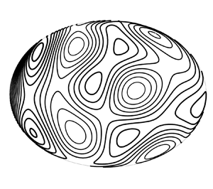
Figure 2. The stream function at  $t=0$ on the (a) sphere, (b) prolate spheroid, (c) oblate spheroid and (d) triaxial ellipsoid. The initial conditions consist of modes of degrees $n=5,6,7$ with randomly assigned amplitudes. Darker contours correspond to larger values.

Figure 3. The vorticity at  $t=2.5$ on the (a) sphere, (b) prolate spheroid, (c) oblate spheroid and (d) triaxial ellipsoid. By this time, the flow is fully turbulent. Darker contours correspond to larger values.
Tables 2 and 3 summarize the results. Table 2 displays the angular momentum components  $\mu _i=M_i/4{\rm \pi}$ per unit area, where $M_i$ is computed from (2.31)–(2.33). Division by area makes the ‘scale size’ of $\mu _i$ order one. Thus, $\mu _i \ll 1$ is insignificant. All of our experiments begin with $\mu _i\approx 0$. The asterisks in table 2 denote angular momentum components that are conserved and should therefore remain zero. Differences from that are caused by accumulated numerical truncation error, which is seen to be quite small. The non-conserved angular momentum components generally increase in P, O and T, but the increase is not monotonic, and sign changes even occur. The sign of the non-conserved components of angular momentum is an accident of the initial conditions.
Table 2. Evolution of  $\mu _i=M_i/4{\rm \pi}$, the angular momenta per unit area, in the numerical experiments. The asterisks denote components that are conserved by the dynamics.

Table 3. The fraction,  $E_n$, of energy in the modes of degree $n$. The energy is initially concentrated in degrees $n=5,6,7$. As time increases, it moves towards the lowest $n$ that is not forbidden by angular momentum conservation.

Table 3 shows the fraction,  $E_n$, of total energy in the modes ‘associated’ with degree $n$. By this, we mean the following: the vorticity and stream function at $(x,y,z)$ on the ellipsoid are first projected onto the unit sphere at $(X,Y,Z)$ and then analysed by projection onto spherical harmonics, in a reverse of the method used to assign initial conditions. The better method would be a spectral analysis in terms of ellipsoidal harmonics themselves. These however are very difficult to calculate. Therefore, the data in table 3 must be regarded as an approximation to the true energy spectrum which is good only to the extent that the spherical harmonics resemble the corresponding ellipsoidal harmonics. The eigenvalues recorded in table 1 suggest that this resemblance is adequate: at our values of $a,b,c$, there is no overlap between the eigenvalues $\lambda _1$, $\lambda _2$, $\lambda _3$ corresponding to $n=1$ and the lowest eigenvalue, $\lambda _4$, corresponding to $n=2$.
Table 3 shows that angular momentum conservation on the sphere prevents energy from entering the three lowest modes. By  $t=120$ – the time required for a fluid particle to circumnavigate the sphere approximately 20 times – fully 92 % of the remaining energy has condensed into $n=2$, but none has crossed the angular-momentum barrier into $n=1$. For the prolate spheroid, 64 % of the energy has crossed into $n=1$ and most of the remainder resides in $n=2$, waiting to cross. The corresponding figures for the oblate spheroid are 40 % and 48 %. The condensation of energy into $n=1$ on the triaxial ellipsoid proceeds more slowly than on either of the two spheroids. At $t=120$, only 19 % of its energy has reached the lowest mode.
Figures 4(a,b) and 4(c,d) show two views of the stream function on the sphere and on the prolate spheroid, respectively, at  $t=120$. The two views are by an infinitely distant observer at (a,c) $y=z=0$ and $x=\infty$, and at (b,d) $y=z=0$ and $x=-\infty$. Thus, the two views offer a complete picture. At this late time, the vorticity strongly resembles the stream function. The sphere exhibits four vortices, which could be anticipated from its dominantly $n=2$ composition (table 3). There is of course no reason why any of these vortices should favour a particular direction on the sphere. At $t=120$, the prolate spheroid exhibits two vortices in keeping with its dominantly $n=1$ composition. As expected, the centres of these two vortices lie in the $xy$-plane. They are analogous to the $Y_1^{\pm 1}$ modes, which, unlike the $Y_1^0$ mode, are not prevented by angular momentum conservation from accumulating turbulent energy. These modes are the lowest modes in the system (table 1) and are therefore the site of Bose–Einstein condensation. The corresponding views of the oblate spheroid and the triaxial ellipsoid (not shown) are less easy to characterize, because the energy of the oblate spheroid at $t=120$ is still about equally divided between $n=1$ and $n=2$ (table 3), and the energy of the triaxial ellipsoid is still dominantly in $n=2$.

Figure 4. Two views of the stream function on the (a,b) sphere and on the (c,d) prolate spheroid at  $t=120$. Darker contours correspond to larger values.
Figure 5 shows the same two views of the stream function on the (a,b) oblate spheroid and on (c,d) the triaxial ellipsoid at the final time,  $t=200$. At $t=200$, 56 % of the energy has reached $n=1$ on the oblate spheroid, and the stream function (figure 5a,b) shows vortices centred on $z=0$, as predicted by theory. The triaxial ellipsoid, with its complete lack of symmetry, shows no such tendency (figure 5c,d).

Figure 5. Two views of the stream function on the (a,b) oblate spheroid and on the (c,d) triaxial ellipsoid at the final time  $t=200.$ Darker contours correspond to larger values.
It is interesting that the prolate spheroid, for which the adjustment to equilibrium is relatively rapid has lowest eigenvalue  $2.480$ (table 1) that is displaced upward from the eigenvalues of the sphere, whereas the lowest eigenvalues of the oblate spheroid and triaxial ellipsoid (respectively $1.680$ and $1.838$) are downwardly displaced. One is tempted to say that the adjustment takes longer if it has farther to go. In all cases, except perhaps that of the sphere, this adjustment is extremely slow, but this agrees with previous results; see especially Dritschel et al. (Reference Dritschel, Qi and Marston2015).
4. Discussion
Angular momentum conservation is irrelevant to two-dimensional turbulence on the plane because typical planar geometries lack the corresponding symmetry property. Only planar domains with a perfectly circular boundary (including the infinite plane) conserve a component of angular momentum.
Kraichnan (Reference Kraichnan1967) statistical mechanics extends easily to the sphere. The planar theory predicts an energy spectrum of the form
 \begin{equation} E_i=\frac{1}{\alpha + \beta k_i^2},\end{equation}
where  $k_i$ is the wavenumber – $k_i^2$ the eigenvalue – of the Fourier component denoted by $i$, and $\alpha$ and $\beta$ are constants determined by the values of the energy and enstrophy. Bose–Einstein condensation corresponds to the limit $\alpha \to -\beta k_{min}^2$ as $k_{max}^2 \to \infty$, where $k_{min}$ is the lowest wavenumber and $k_{max}$ the highest wavenumber in the system. (Equilibrium statistical mechanics applies only to a finite set.) For the sphere,
 \begin{equation} E_n^m=\frac{1}{\alpha + \beta n(n+1)},\end{equation}
but this applies only to  $n\ne 1$. On the sphere, the constants $\alpha$ and $\beta$ are again defined by the values of energy and enstrophy, but for this purpose, the sums in (2.46a,b) must exclude the $n=1$ modes, whose contributions are not allowed to change. From the standpoint of statistical mechanics, $\psi _1^m$ and $q_1^m$ are constants and are statistically sharp. This point was emphasized in the pioneering calculation of Frederiksen & Sawford (Reference Frederiksen and Sawford1980). For the non-spherical ellipsoids, the situation is slightly more complicated in that the angular momentum does not correspond to a single ellipsoidal harmonic, but for ellipsoids that are leading order spherical, the angular momentum modes are leading order spherical harmonics.
Strictly speaking, equilibrium statistical mechanics applies only to the inviscid case. In the inviscid case, enstrophy piles up near the highest allowed wavenumber (i.e. largest eigenvalue) in the system, and disappears to infinity as that wavenumber is increased. Numerical computation is impractical for  $k_{max} \to \infty$, but moderate viscosity removes enstrophy from the wavenumbers near $k_{max}$ much as if that enstrophy had migrated to unresolved scales. Moreover, by smoothing the flow at the smallest resolved scales, viscosity prevents spatial truncation error from destroying angular momentum conservation. (In our numerical model, the Jacobian dynamics conserves energy and enstrophy despite the truncation error arising from finite grid size, but angular momentum is conserved only to within spatial truncation error.) The general agreement of our results with the predictions of equilibrium statistical mechanics is both a vindication of the theory and a proof of the accuracy of our code.
Earth is an oblate spheroid whose departure from sphericity is much smaller than the spheroids considered in § 3. It corresponds to  $a=b=1$ and $c=1-1/298$. To this spheroid we have applied the same initial conditions as in § 3 and found no very significant departures from the spherical experiment for times out to $t=320$. The difficulty is in distinguishing the effects of very small oblateness from the noise of accumulated numerical truncation error, which also grows slowly as time increases.
Meteorologists have long been aware of torques arising from Earth's lack of rotational symmetry, but they adopt a somewhat different viewpoint to that adopted here. In their budget of exact angular momentum (defined similarly to (2.28)), oblateness enters as one of several torques and is sometimes called ‘flatness torque’ or ‘bulge torque’. See Egger et al. (Reference Egger, Weichmann and Hoinka2007) for an extensive review. Other torques include those arising from mountain topography and from gravitational force. Neither of the latter are present in our dynamics. Much of the meteorological work is based upon observations, and it is applied to much more realistic dynamics than the two-dimensional incompressible flow considered by us. Thus, the relevance of the present study to Earth's atmosphere is unclear.
The choice of dynamics is critical. In their calculation of the statistical mechanics of barotropic flow on a rotating sphere with mountain topography, Sawford & Frederiksen (Reference Sawford and Frederiksen1983) adopt quasi-geostrophic dynamics, in which the topography term contains a factor of Coriolis parameter (their  $\mu = \sin \theta$). If one were to regard the equatorial bulge as a form of mountain topography, then their calculation would predict a response only if there were non-vanishing $M_3$ (i.e. non-vanishing Coriolis parameter). In our dynamics on the spheroid, $M_1$ and $M_2$ increase regardless of the value of $M_3$, which, as in our experiments, may vanish.
The sphere seems to be the ideal geometry in which to study pure two-dimensional turbulence. It has no boundary, and, if  $\boldsymbol {M}=0$, it has no preferred direction.
Acknowledgements
We thank three anonymous referees for helpful comments.
Funding
N. Pizzo was partially supported by grant NSF OCE-2219752 and NASA SMODE 80NSSC19K1037.
Declaration of interests
The authors report no conflict of interest.


 Open access