


1. Introduction
Boundary layers subjected to favourable pressure gradients (FPGs) or adverse pressure gradients (APGs) are common in fluid engineering. In the past 30 years, many have studied boundary layers with pressure gradients, including theory work (Perry, Marusic & Jones Reference Perry, Marusic and Jones1998; Nickels Reference Nickels2004; Wei, Fife & Klewicki Reference Wei, Fife and Klewicki2007; Wei, Maciel & Klewicki Reference Wei, Maciel and Klewicki2017; Subrahmanyam, Cantwell & Alonso Reference Subrahmanyam, Cantwell and Alonso2022), experimental work (Aubertine & Eaton Reference Aubertine and Eaton2005; Harun et al. Reference Harun, Monty, Mathis and Marusic2013; Volino Reference Volino2020; Parthasarathy & Saxton-Fox Reference Parthasarathy and Saxton-Fox2022; Romero et al. Reference Romero, Zimmerman, Philip, White and Klewicki2022b) and computational work (Lee & Sung Reference Lee and Sung2009; Inoue et al. Reference Inoue, Pullin, Harun and Marusic2013; Kitsios et al. Reference Kitsios, Sekimoto, Atkinson, Sillero, Borrell, Gungor, Jiménez and Soria2017; Lee Reference Lee2017; Subrahmanyam et al. Reference Subrahmanyam, Xu, Cantwell and Alonso2023), to name a few of the previous works. It was known that the mean flow responds to pressure gradients faster than the turbulence. It has also been found that there are history effects, and the law of the wall loses its predictive power. However, it is unclear how one can account for history effects in a mean flow scaling. Consequently, no good mean flow scaling exists for boundary layers with pressure gradients. This work aims to account for history effects in the mean flow scaling and establish a universal mean flow scaling for boundary layers subjected to arbitrary APGs and FPGs.
We begin our discussion by estimating the pressure gradients encountered in engineering flows. Consider, for example, the boundary layer on the suction side of an aerofoil, such as sterns on an underwater vehicle or a turbine blade. At large angles of attack, the pressure gradient causes an appreciable change in the fluid velocity. An order-of-magnitude estimate of the pressure gradient is
 \begin{equation} \left|\frac{{\rm d} P}{{\rm d} s}\right|=\alpha\,\frac{\rho U_0^2}{ c}, \end{equation}
where  ${\rm d} P/{\rm d} s$ is the pressure gradient along a streamline, $U_0$ is the velocity of the incoming fluid, $c$ is the chord length, and $\alpha$ is an order 0.1 factor. Define
 \begin{equation} \varPi\equiv\frac{\delta}{\rho\tau_w}\left|\frac{{\rm d} P}{{\rm d} s}\right|, \end{equation}
where  $\delta$ is the boundary layer thickness, and $\tau _w=\nu \,{\rm d} U/{{\rm d}y}$ is the wall-shear stress. We have
 \begin{equation} \varPi=\frac{\delta}{\rho\tau_w}\,\frac{\alpha \rho U_0^2}{c}=\frac{2 \alpha \delta/c}{C_f}. \end{equation}
A rough estimate according to Anderson (Reference Anderson2011) is
 \begin{equation} C_f\sim O(10^{-4}\unicode{x2013}10^{-3}),\quad \alpha \delta/c\sim O(0.001\unicode{x2013}0.01), \end{equation}
which leads to
 \begin{equation} \varPi\sim O(1)\text{ to }O(100). \end{equation}
Following this estimate, we limit ourselves to  $|\varPi |$ between 1 and 100. Flows subjected to a pressure gradient with $\varPi <1$ will be in a quasi-equilibrium state, and flows subjected to a pressure gradient with $\varPi >100$ are rare.
Consider the scaling of the mean velocity. The canonical law of the wall (LoW) provides a good working approximation of the mean flow in a zero pressure gradient (ZPG) boundary layer. Here, the LoW refers to the scaling of the mean flow in the constant stress layer (or the inner layer), where the inner scaled velocity follows a linear and a logarithmic scaling of the inner scaled distance from the wall for  $y\lesssim 5\nu /u_\tau$ and $\nu /u_\tau \ll y\ll \delta$, respectively:
 \begin{equation} \left.\begin{gathered} U^+=y^+ \quad \text{for}\ y\lesssim 5\nu/u_\tau,\\ U^+=\frac{1}{\kappa}\log(y^+)+B\quad \text{for}\ \nu/u_\tau\ll y\ll \delta. \end{gathered}\right\} \end{equation}
The behaviour of the mean flow in the buffer layer is also a function of  $y^+$ only, but there is no accepted explicit expression. Here, $U^+=U/u_\tau$, where $U$ is the mean velocity, $u_\tau$ is the friction velocity, $y^+=yu_\tau /\nu$, $\nu$ is the kinematic viscosity, $y$ is the wall-normal coordinate, $\delta$ is an outer length scale (e.g. boundary layer thickness, half-channel height, pipe radius), $\kappa \approx 0.4$ is the von Kármán constant (keeping only one significant digit), and $B\approx 5$ is a constant (Kim, Moin & Moser Reference Kim, Moin and Moser1987; Monty et al. Reference Monty, Hutchins, Ng, Marusic and Chong2009; Smits, McKeon & Marusic Reference Smits, McKeon and Marusic2011; Marusic et al. Reference Marusic, Monty, Hultmark and Smits2013; Morrill-Winter, Philip & Klewicki Reference Morrill-Winter, Philip and Klewicki2017). Equation (1.6) fails when the boundary layer is subjected to a strong pressure gradient (Spalart & Watmuff Reference Spalart and Watmuff1993; Nagib & Chauhan Reference Nagib and Chauhan2008; Monty, Harun & Marusic Reference Monty, Harun and Marusic2011). For illustrative purposes, consider the model problem sketched in figure 1(a), where a fully developed channel is subjected to a suddenly imposed APG. Figure 1(b) shows the velocity profiles in inner units, at a few time instants after an APG $\varPi =100$ is imposed suddenly on a $Re_{\tau,0}=u_{\tau,0}\delta /\nu =1000$ channel. Beside that the velocity is above the log law, the region within which $U^+=y^+$ also retreats, which is quite peculiar. We discuss the scaling of the mean flow in the viscous sublayer in Appendix A. Define
 \begin{equation} \Delta p^+ \equiv \frac{\nu}{\rho u_{\tau}^3}\, \frac{{\rm d} P}{{\rm d}\kern 0.06em x}\quad \text{and}\quad \beta\equiv\frac{\delta^*}{\rho u_{\tau}^2}\,\frac{{\rm d} P}{{\rm d}\kern 0.06em x}, \end{equation}
which are common non-dimensional measures of the APG, with  $\beta$ being the Clauser pressure gradient coefficient, $\delta ^*$ being the displacement height, and $\rho$ being the fluid density. The displacement height in a channel flow is defined as
 \begin{equation} \delta^*=\int_0^\delta \left(1-\frac{U}{U_c}\right){{\rm d}y}, \end{equation}
where  $\delta$ is the half-channel height, and $U_c$ is the mean streamwise velocity at the centreline. Here, the Clauser parameter is the ratio of the two quantities that cause the momentum thickness to increase in a spatially developing boundary layer (in the momentum integral equation). We will report both $\Delta p^+$ (Nickels Reference Nickels2004; Johnstone, Coleman & Spalart Reference Johnstone, Coleman and Spalart2010; Lozano-Durán et al. Reference Lozano-Durán, Giometto, Park and Moin2020; Knopp et al. Reference Knopp, Reuther, Novara, Schanz, Schülein, Schröder and Kähler2021) and $\beta$ in the following for completeness. For this model problem, $\Delta p^+=0.1$, $\beta =11.6$ at the initial state.

Figure 1. (a) Schematic of the model problem. A fully developed channel is subjected to a suddenly imposed APG and decelerates as a result. (b) Mean velocity profiles at a few time instants. The flow is initially at a Reynolds number  $Re_\tau =1000$. An APG $\varPi =+100$ is imposed at $t=0$. Shown here are velocity profiles at $t u_{\tau,0}/\delta =0.005$ (blue), 0.035 (red) and 0.065 (yellow). The profiles are normalized with the density $\rho$, viscosity $\mu$ and instantaneous wall shear stress $\tau _w(t)$. The dashed lines correspond to (1.6), but we allow $\kappa$ and $B$ in (1.6) to vary. Best fits yield $\kappa =0.35, 0.23, 0.079$ and $B=5.8, 5.48, 9.2$ at $t u_{\tau,0}/\delta =0.005, 0.035, 0.065$, respectively.
We see clear history effects in figure 1(b): the same force leads to different velocity profiles at different time instances. This is quite expected: since  $F=ma$ and $Ft=m\,\Delta V$, the change in the fluid velocity is determined not solely by the instantaneous force but by the force acting on the fluid parcel for a period of time. Such history effects were also noted in Perry, Marusic & Jones (Reference Perry, Marusic and Jones2002), Bobke et al. (Reference Bobke, Vinuesa, Örlü and Schlatter2017), Volino (Reference Volino2020) and Romero et al. (Reference Romero, Zimmerman, Philip, White and Klewicki2022b), among others. We see from figure 1(b) that the LoW in (1.6) with $\kappa =0.4$ and $B=5$ does not fit the data, not even the lower part of the velocity profiles, which is in contrast to Galbraith, Sjolander & Head (Reference Galbraith, Sjolander and Head1977), Perry (Reference Perry1966) and Spalart & Watmuff (Reference Spalart and Watmuff1993). By varying the two ‘constants’ in the log law, (1.6) fits the mean flow in the inner layer (Nagib & Chauhan Reference Nagib and Chauhan2008; Lee & Sung Reference Lee and Sung2009; Knopp et al. Reference Knopp, Reuther, Novara, Schanz, Schülein, Schröder and Kähler2021), as indicated by the black dashed lines in figure 1. Here, the inner layer is the layer where the outer length scale does not play a role. In most studies, this layer is considered as $y\lesssim 0.15\delta$. However, tuning $\kappa$ and $B$ to fit data reduces the modelling task to a fitting exercise. The same can be said about the half power law (Stratford Reference Stratford1959; Perry & Schofield Reference Perry and Schofield1973; Knopp et al. Reference Knopp, Reuther, Novara, Schanz, Schülein, Schröder and Kähler2021) and other laws (Perry Reference Perry1966; Perry, Bell & Joubert Reference Perry, Bell and Joubert1966; Ding et al. Reference Ding, Saxton-Fox, Hultmark and Smits2019; Subrahmanyam et al. Reference Subrahmanyam, Cantwell and Alonso2022) where one must also adjust the ‘constants’ to fit data. Although the LoW also contains constants, i.e. $\kappa$ and $B$, that must be calibrated against data, the fact that one does not need to adjust these two constants as a function of the Reynolds number makes the LoW ‘universal’.
This work aims to establish a universal mean velocity scaling for wall-bounded flows subjected to arbitrary streamwise pressure gradients. Here, universality is with respect to the pressure gradient and its history. Mean flow scalings are usually explicit algebraic relations with the normalized velocity on the left-hand side and the dependent variables on the right-hand side (Volino Reference Volino2020; Romero et al. Reference Romero, Zimmerman, Philip and Klewicki2022a). If we were to follow this path, we would be looking for a scaling for  $U$ as a function of the inner and outer length scales and the history of the pressure gradients, which is a daunting task. Instead, we will pursue the idea of velocity transformation. This idea has received much attention in the high-Mach-number-flow literature (Huang & Coleman Reference Huang and Coleman1994; Trettel & Larsson Reference Trettel and Larsson2016; Volpiani et al. Reference Volpiani, Iyer, Pirozzoli and Larsson2020; Griffin, Fu & Moin Reference Griffin, Fu and Moin2021). The goal of these transformations is to find $U_m$ and $L_m$,
 \begin{equation} U^*=\int_{0}^{U}\frac{1}{U_m}\,{\rm d} U,\quad y^*=\int_{0}^{y}\frac{1}{L_m}\,{\rm d} y, \end{equation}
such that the transformed velocity  $U^*$ follows the LoW and is a function of $y^*$ irrespective of the density variation in the flow (Van Driest Reference Van Driest1951; Modesti & Pirozzoli Reference Modesti and Pirozzoli2019; Modesti, Pirozzoli & Grasso Reference Modesti, Pirozzoli and Grasso2019). We have a similar goal, but instead of equilibrium boundary layers, we study non-equilibrium boundary layers subjected to streamwise pressure gradients. The objective is to find a transformation such that the transformed velocity $U^*$ follows the LoW and is a function of $y^*$ only, irrespective of the pressure gradient.
The rest of the paper is organized as follows. We derive the transformation in § 2. Details of the validation direct numerical simulations (DNS) data are presented in § 3, followed by test results in § 4. Finally, we conclude in § 5.
2. Velocity transformation
In this section, we derive the velocity transformation from the Navier–Stokes equation and discuss its properties.
2.1. Assumptions
The derivation assumes the following. First, the flow is incompressible. Second, the mean flow is two-dimensional. This holds when the pressure gradients are in the streamwise direction. Third, the boundary layer is thin with respect to its rate of growth. That is, the velocity gradient in the wall-normal direction is much larger than that in the streamwise direction (which is only approximately true for boundary layers but is exactly true for channel flow). This assumption limits the discussion to attached flows, i.e. before incipient separation. Fourth, the flow is assumed to be initially in an equilibrium state. That is, the mean flow initially conforms to the LoW. Fifth, it is assumed that a universal velocity transformation exists. Define
 \begin{equation} f\equiv \frac{{\rm d} U^*}{{\rm d} y^*}\,(1+\nu_t^+). \end{equation}
Here,  $\nu _t^+=\nu _t/\nu$, where $\nu$ is the kinematic viscosity, $\nu _t=-\langle uv\rangle /(\textrm {d} U/\textrm {d} y)$ is the eddy viscosity, and $-\langle uv\rangle$ is the Reynolds shear stress. By universality, $f$ is a function of $y^*$ only in the inner layer. Like any assumption in any theory, (2.1) facilitates mathematical derivations, and its validity must be verified empirically.
Since the transformed velocity  $U^*$ is a function of the transformed wall-normal coordinate $y^*$ only, it follows from this universality assumption that $\nu _t^+$ is also a function of only $y^*$ only in the inner layer. In addition, because $f=1$ in the inner layer of ZPG boundary layer flows (due to the constant stress layer), the universality assumption implies that $f\equiv 1$ in all flows – in the layer where the outer length scale does not play a role. Note that we do not need to assume a constant stress layer. The function $f$, in general, is a function of $y/\delta$.
2.2. Governing equation
The Reynolds-averaged streamwise momentum equation reads
 \begin{equation} \frac{\partial U}{\partial t}+U\,\frac{\partial U}{\partial x}+V\, \frac{\partial U}{\partial y}=-\frac{1}{\rho}\,\frac{\partial P}{\partial x}+ \frac{\partial \tau_{xx}}{\partial x}+\frac{\partial \tau_{xy}}{\partial y}, \end{equation}
where
 \begin{equation} \tau_{xx}=2\nu\,\frac{\partial U}{\partial x}-\left\langle u'u'\right\rangle,\quad \tau_{xy}=\nu\left(\frac{\partial U}{\partial y}+\frac{\partial V}{\partial x}\right)- \left\langle u'v'\right\rangle. \end{equation}
The equation assumes incompressibility and two-dimensional mean flow. Hence the  $\partial /\partial z$ terms are dropped. Here, the uppercase letters denote mean quantities, the lowercase letters denote instantaneous quantities, $'$ denotes fluctuations, $x$,
$x$,  $y$ and $z$ are the streamwise, wall-normal and spanwise directions, $U, V, W$ or $u, v, w$ give the velocity in the three Cartesian directions, $\boldsymbol{\tau}$ is the stress, and $\langle {\cdot }\rangle$ denotes ensemble averaging. Invoking the thin boundary layer assumption leads to
 \begin{equation} \frac{\partial V}{\partial x}\ll\frac{\partial U}{\partial y},\quad \frac{\partial \tau_{xx}}{\partial x}\ll\frac{\partial \tau_{xy}}{\partial y}. \end{equation}
It follows from (2.2), (2.3a,b) and (2.4a,b) that
 \begin{equation} \frac{\partial U}{\partial t}+U\,\frac{\partial U}{\partial x}+V\,\frac{\partial U}{\partial y}=-\frac{1}{\rho}\, \frac{\partial P}{\partial x}+\frac{\partial \tau_{xy}}{\partial y}, \end{equation}
where
 \begin{equation} \tau_{xy}=\nu\,\frac{\partial U}{\partial y}-\left\langle u'v'\right\rangle. \end{equation}
We take the  $y$ derivative of both sides of (2.5):
 \begin{equation} \left(\frac{\partial }{\partial t} + U\,\frac{\partial }{\partial x}+V\, \frac{\partial }{\partial y}\right)\frac{\partial U}{\partial y}+ \frac{\partial U}{\partial y}\,\frac{\partial U}{\partial x}+ \frac{\partial V}{\partial y}\,\frac{\partial U}{\partial y}=-\frac{1}{\rho}\, \frac{\partial^2 P}{\partial x\,\partial y}+\frac{\partial^2 \tau_{xy}}{\partial y^2}. \end{equation}
We seek to simplify (2.7). First, incompressibility requires
 \begin{equation} \frac{\partial U}{\partial x}+ \frac{\partial V}{\partial y}=0. \end{equation}
Second, the  $y$ momentum equation reads:
 \begin{equation} \frac{1}{\rho}\,\frac{\partial P}{\partial y}+ \frac{\partial \left\langle v^2\right\rangle}{\partial y}=0. \end{equation}
By applying  $\partial /\partial x$ on both sides of (2.9), we have
 \begin{equation} \frac{1}{\rho}\,\frac{\partial^2 P}{\partial x\,\partial y}= \frac{\partial^2 \left\langle v^2\right\rangle}{\partial x\,\partial y}\ll \frac{\partial^2 \tau_{xy}}{\partial y^2}, \end{equation}
due to the thin boundary layer assumption. Substituting (2.8) and (2.10) into (2.7) leads to
 \begin{equation} \frac{{{\rm D}}}{{\rm D} t}\,\frac{\partial U}{\partial y}=\frac{\partial^2 \tau_{xy}}{\partial y^2}. \end{equation}
 Invoking the eddy viscosity  $\nu _t$, the shear stress term is
 \begin{equation} \tau_{xy}=\nu\,\frac{\partial U}{\partial y}\left(1+\nu_t^+\right). \end{equation}
Here,  $\nu _t$ is unspecified. Hence invoking $\nu _t$ introduces no modelling error. Plugging (1.9a,b) and (2.1) into (2.12), we have
 \begin{equation} \frac{\nu}{\tau_{xy}}\,\frac{U_m}{L_m}\,f=1. \end{equation}
2.3. Transformation
Equations (1.9a,b) and (2.13) lead to
 \begin{equation} U^*=\int_0^U \frac{\nu f}{\tau_{xy}}\,\frac{{\rm d} y^*}{{\rm d} y}\,{\rm d} U. \end{equation}
Equation (2.14) is a velocity transformation, but it requires knowledge of  $y^*$. In the following, we derive a transformation that maps $y^+$ to $y^*$.
Integrating (2.11) in time, we have
 \begin{equation} \frac{\partial U}{\partial y}=\left(\frac{\partial U}{\partial y}\right)_0+ \int_0^t\frac{\partial^2 \tau_{xy}}{\partial y^2}\,{\rm D} t, \end{equation}
where the subscript  $0$ denotes quantities evaluated at the initial state. Note that the integration is Lagrangian. Invoking the assumed initial state, the mean flow abides by the LoW, therefore,
 \begin{equation} \left(\frac{\partial U}{\partial y}\right)_0=\left(\frac{u_\tau^2}{\nu}\, \frac{1}{F(y^+)}\right)_0=\frac{u_{\tau,0}^2}{\nu}\,\frac{1}{F(y_0^+)}, \end{equation}
where
 \begin{equation} F(y_0^+)=1+\kappa y_0^+\left(1-\exp(-y_0^+{/}A)\right)^2 \end{equation}
is a damping function (Van Driest Reference Van Driest1956; Kawai & Larsson Reference Kawai and Larsson2012; Yang & Lv Reference Yang and Lv2018),  $A=17$ is a constant, $y_0^+=yu_{\tau,0}/\nu$, and $u_{\tau,0}$ is the friction velocity at the initial state. The use of the van Driest damping function is to give the equilibrium $\partial U/\partial y$ a closed expression. The derivation itself does not necessarily need such an approximation. An alternative definition for $F$ is
 \begin{equation} F(y^+_0)=\frac{u_{\tau,0}^2}{\nu}\,\frac{1}{\left({\partial U}/{\partial y}\right)_0}, \end{equation}
where we have left  $\left ({\partial U}/{\partial y}\right )_0$ as is. Invoking (2.13) and the assumption that $U^*$ follows the LoW, the left-hand side of (2.15) is
 \begin{equation} \frac{\partial U}{\partial y}=\frac{\tau_{xy}}{\nu f}\,\frac{1}{F(y^*)}. \end{equation}
Substituting (2.19) into (2.15) and rearranging, we have
 \begin{equation} {F(y^*)=\frac{1}{\left(\dfrac{\partial U}{\partial y}\right)_0+ \displaystyle\int_0^t\dfrac{\partial^2 \tau_{xy}}{\partial y^2}\,{\rm D} t}\,\frac{\tau_{xy}}{\nu f}.} \end{equation}
Here,  $F$ is given in (2.17), $f\equiv 1$ for $y\ll \delta$, its value in the outer layer can be measured at the initial state (as a function of $y/\delta$), and the derivative $(\partial U/\partial y)_0$ is known from the equilibrium LoW. Equations (2.20) and (2.14) are the transformations that we are looking for.
2.4. Further simplification
We rearrange (2.20) and (2.14) to put them into the standard form as defined in (1.9a,b). First, we define
 \begin{equation} g\equiv\frac{\partial U/\partial y-\left(\partial U/\partial y\right)_0}{\left(\partial U/\partial y\right)_0}. \end{equation}
It follows from (2.15), (2.16) and (2.21) that
 \begin{equation} g=\frac{\nu\,F(y^+_0)}{u_{\tau,0}^2} \int_0^t\frac{\partial^2 \tau_{xy}}{\partial y^2}\,{\rm D} t. \end{equation}
Equations (2.22) and (2.20) together give
 \begin{equation} y^*=F^{-1}\left[\frac{1+g_w}{1+g}\,\frac{\tau^+}{f}\,F(y_0^+)\right]. \end{equation}
Here,  $F^{-1}$ denotes the inverse function of $F$,
$F$,  $\tau ^+=\tau _{xy}/\tau _{xy,w}$, and $g_w$ is $g$ evaluated at the wall. Notice that $\tau ^+$ is ill-defined at separation, therefore our scaling is valid up to incipient separation. The term $(1+g_w)/(1+g)$ in (2.23) accounts for the history effects. Equation (2.23) gives
 \begin{equation} y^*=\int_0^y \frac{F(y^*)}{F'(y^*)}\left[\frac{f}{\tau^+}\, \frac{\partial}{\partial y}\left(\frac{\tau^+}{f}\right) - \frac{1}{1+g}\,\frac{\partial g}{\partial y} + \frac{F'(y^+_0)}{F(y^+_0)}\, \frac{{\rm d} y_0^+}{{\rm d} y}\right] {\rm d} y. \end{equation}
Equations (2.24) and (2.14) give
 \begin{equation} U^*=\int_0^U \frac{\nu f}{\tau_{xy}}\,\frac{F(y^*)}{F'(y^*)} \left[\frac{f}{\tau^+}\,\frac{\partial}{\partial y}\left(\frac{\tau^+}{f}\right) - \frac{1}{1+g}\,\frac{\partial g}{\partial y} + \frac{F'(y^+_0)}{F(y^+_0)}\, \frac{{\rm d} y_0^+}{{\rm d} y}\right] {\rm d} U. \end{equation}
Equations (2.24) and (2.25) are the velocity transformation.
2.5. Discussion
The transformations are collected below:
 \begin{equation} \left.\begin{gathered} y^*=\int_0^y \frac{F(y^*)}{F'(y^*)}\left[ \frac{f}{\tau^+}\,\frac{\partial}{\partial y} \left(\frac{\tau^+}{f}\right) - \frac{1}{1+g}\,\frac{\partial g}{\partial y} + \frac{F'(y^+_0)}{F(y^+_0)}\,\frac{{\rm d} y_0^+}{{\rm d} y}\right] {\rm d} y,\\ U^*=\int_0^U \frac{\nu f}{\tau_{xy}}\,\frac{F(y^*)}{F'(y^*)}\left[\frac{f}{\tau^+}\, \frac{\partial}{\partial y}\left(\frac{\tau^+}{f}\right) - \frac{1}{1+g}\, \frac{\partial g}{\partial y} + \frac{F'(y^+_0)}{F(y^+_0)}\,\frac{{\rm d} y_0^+}{{\rm d} y}\right] {\rm d} U. \end{gathered}\right\} \end{equation}
We have the following remarks. First, the transformation accounts for history effects through the time integral  $g$. It is interesting to note that the integral is not weighted, therefore the flow does not ‘forget’. In other words, an event at $t=0$ and an event at a later time instant contribute equally to the transformation. Second, the transformation is valid in the outer layer as well. The function $f$ is 1 in the inner layer and varies as a function of $y/\delta$ outside. By measuring $f$ from the initial condition as a function of $y/\delta$, the transformation should collapse all velocity profiles. Hence the transformation avoids the constant stress layer assumption, at least formally. Third, the transformation is presented as a descriptive tool for now. The transformation shows how history should be accounted for in mean flow scalings. It shows that pressure gradients do not affect the mean flow directly. Instead, they affect the shear stress $\tau _{xy}$, which then affects the mean flow. Closures for $\tau _{xy}$ and $\nu _t^+$ are needed for the transformation, a topic that we do not discuss here. Fourth, the transformation involves a function inverse and therefore is not explicit.
In the following, we simplify and rewrite the transformation for the log layer in a ZPG boundary layer, for Couette–Poiseuille flow, for a channel with a suddenly imposed streamwise pressure gradient, and for spatially developing boundary layers with streamwise pressure gradients.
First, for the log and the viscous layers, we have
 \begin{equation} \tau_{xy}={\rm const}. \end{equation}
It follows that  $g=0$ and $\tau ^+/f=1$. Hence for flows in the constant stress layer, the velocity transformation reduces to $U^*=U^+$ and $y^*=y^+$.
Second, we consider the Couette–Poiseuille flow. Figure 2(a) shows a schematic of the flow. The flow is subjected to an APG near one wall and an FPG near the other. The stress  $\tau _{xy}$ is a linear function of $y$. The function $f$ can be measured from the Couette flow, and $f=1$. It follows that $g=0$, therefore (2.23) becomes
 \begin{equation} F(y^*)=\tau^+\,F(y^+). \end{equation}
The velocity transformation becomes
 \begin{equation} U^*=\int_0^U \frac{\nu f}{\tau_{xy}}\,\frac{F(y^*)}{F'(y^*)} \left(\frac{1}{\tau^+}\,\frac{\partial \tau^+}{\partial y}+ \frac{F'(y^+)}{F(y^+)}\,\frac{{{\rm d}y}^+}{{\rm d}y}\right) {\rm d} U. \end{equation}
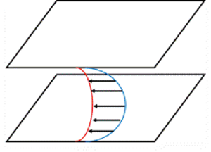
Figure 2. (a) A sketch of Couette–Poiseuille flow. The flow is subjected to an FPG near the top plate and an APG near the bottom plate (Johnstone et al. Reference Johnstone, Coleman and Spalart2010; Coleman & Spalart Reference Coleman and Spalart2015). (b) A sketch of a boundary layer subjected to APGs. The pressure gradient (PG) is imposed by varying the freestream velocity. The reader is directed to Bobke et al. (Reference Bobke, Vinuesa, Örlü and Schlatter2017) for more details.
Third, for channel flow with a suddenly imposed streamwise pressure gradient, the mean advection is 0, therefore the Lagrangian integration degenerates to an Eulerian one, i.e.  $\textrm {D} t=\textrm {d} t$. It follows that (2.22) becomes
 \begin{equation} g=\frac{\nu\,F(y^+_0)}{u_{\tau,0}^2} \int_0^t\frac{\partial^2 \tau_{xy}}{\partial y^2}\,{\rm d} t,\quad y>0. \end{equation}
Furthermore, measuring  $f$ from the initial condition, we have $f=1-y/\delta$.
Fourth, for a spatially developing turbulent boundary layer with streamwise pressure gradients, Lagrangian integration is along the streamline, and (2.22) becomes
 \begin{equation} g=\frac{\nu\,F(y^+_0)}{u_{\tau,0}^2} \int_0^t\frac{\partial^2 \tau_{xy}}{\partial y^2}\, \frac{{\rm d} s}{\left|\boldsymbol{U}\right|},\quad y > 0, \end{equation}
where  $\textrm {d} s$ is along a streamline, and $|\boldsymbol {U}|$ is the velocity magnitude. Equation (2.31) is singular at the wall because of the no-slip condition. However, this singularity is removable. We know that the velocity follows $U^+=y^+$ sufficiently close to the wall, irrespective of any non-equilibrium effects. Since $U^*$ is a universal function of $y^*$, we must have $U^*=y^*$ sufficiently close to the wall as well. This gives directly $y^*=y^+$ at the wall, thereby removing the singularity at the wall.
3. Computational set-up
To test the velocity transformation, we conduct DNS of channel flows subjected to a suddenly imposed APG or FPG. The flow is sketched in figure 1(a). It is a fully developed two-dimensional turbulent channel. At  $t=0$, a constant pressure gradient $\textrm {d} P/{\textrm {d}\kern0.06em x}$ is imposed suddenly, and subsequently held constant for the duration of the simulation. The mean flow evolves with time as a result.
Table 1 shows the DNS details. The nomenclature is as follows:  $R[Re_{\tau,0}/100]\,F/A[|\varPi |]$, where $F$ is for FPG, and $A$ is for APG. For APGs, $\varPi$ is $1$,
$1$,  $10$ or $100$, corresponding to a weak APG, a moderate APG, and a strong APG. For FPGs, $\varPi =-10$ or $-$100, corresponding to a moderate or strong FPG. FPGs are not very challenging (or interesting) because the canonical LoW works reasonably well for flows with FPGs (Townsend Reference Townsend1956; Mellor & Gibson Reference Mellor and Gibson1966), although FPGs have interesting effects on the eddies in the flow (Volino Reference Volino2020). The initial Reynolds number is $Re_{\tau,0}=544$ or 1000. The Reynolds number increases when an FPG is applied and decreases when an APG is applied. The size of the channel is $(4{\rm \pi} \times 2 \times 2{\rm \pi} )\delta$ for the R5 ( $Re_{\tau,0}=544$) cases, and $(8{\rm \pi} \times 2 \times 3{\rm \pi} )\delta$ for the R10 ( $Re_{\tau,0}=1000$) cases. The domain sizes for the R5 and R10 cases are different because the initial fields were generated by different authors. Nonetheless, both domains are larger than that of the minimal channel (Lozano-Durán & Jiménez Reference Lozano-Durán and Jiménez2014). The grid resolution is comparable to that in Mathur et al. (Reference Mathur, Gorji, He, Seddighi, Vardy, O'Donoghue and Pokrajac2018) and Yang et al. (Reference Yang, Hong, Lee and Huang2021), and is such that the flow is well-resolved from the beginning to the end. We employ statistically uncorrelated initial flow fields, and repeat the simulations multiple times to get converged statistics following Lozano-Durán et al. (Reference Lozano-Durán, Giometto, Park and Moin2020), Chung (Reference Chung2005) and He & Seddighi (Reference He and Seddighi2015). The code that we use is the same as in Lee & Moser (Reference Lee and Moser2015). Details of the code can be found in Graham et al. (Reference Graham2016) and Lee & Moser (Reference Lee and Moser2015), and are not detailed here for brevity.
Table 1. DNS details of channel flows subjected to a suddenly imposed adverse ( $\varPi >0$) or favourable ( $\varPi <0$) pressure gradient. Here, $Re_{\tau,0}$ is the initial Reynolds number; $\varPi$ is positive for APG and negative for FPG; $L_x$, $L_y$ and $L_z$ are the domain sizes in the streamwise, wall-normal and spanwise directions. Normalization is by the half-channel height. Also, $n_x$, $n_y$ and $n_z$ are the numbers of grid points in the three Cartesian directions, and $\Delta x^+$, $\Delta y^+$ and $\Delta z^+$ are the grid spacings in the three directions. For $\Delta y^+$, we list the resolution at the wall and the channel centre. We list the grid resolution at the beginning or the end of the DNS. For $\varPi >0$, a finer grid must be employed at the beginning than at the end, and we list the grid resolution at the beginning of the DNS, and vice versa. Parameter $N$ is the number of ensembles used to compute the flow statistics.

We will also use the boundary layer data in Bobke et al. (Reference Bobke, Vinuesa, Örlü and Schlatter2017), and the Couette–Poiseuille data in Coleman & Spalart (Reference Coleman and Spalart2015) and Johnstone et al. (Reference Johnstone, Coleman and Spalart2010). The flows are sketched in figure 2. Flow parameters that are relevant to this analysis are tabulated in table 2. Further details are not shown here for brevity.
Table 2. Details of the Couette–Poiseuille (CP) flows and the boundary layer (BL) flows. The nomenclature is [Initial of authors][ $Re_\tau /100$][PG], where $Re_\tau$ is the friction Reynolds number. Further details of the flows can be found in Coleman, Garbaruk & Spalart (Reference Coleman, Garbaruk and Spalart2015) and Johnstone et al. (Reference Johnstone, Coleman and Spalart2010), and are not repeated here for brevity. The velocity in a Couette–Poiseuille flow increases monotonically from one wall to the other. It is therefore not straightforward to define the heights of the boundary layers near the two walls. Consequently, defining $\beta$ is not straightforward for Couette–Poiseuille flow. The nomenclature of the BL cases is the same as in Bobke et al. (Reference Bobke, Vinuesa, Örlü and Schlatter2017). The ranges of $Re_\tau$ and $\varPi$ are shown in the table. Note that for cases b1 and b2, $\varPi$ is approximately a constant, while for cases m13, m16 and m18, it is varying. We also include the ZPG-BL data in Schlatter & Örlü (Reference Schlatter and Örlü2010) for comparison purposes.

4. Results
4.1. Channel flow results
First, we present the channel flow results. Figures 3 and 4 show the mean velocity profiles in the APG cases. Figure 3 shows the R5 results, and figure 4 shows the R10 results. The results at other time instants are similar and are not shown here for brevity. In R5A1, a weak APG is applied, and the flow is at a quasi-equilibrium state. As a result, both  $U^+$ and $U^*$ follow the LoW. In R5A10 and R10A10, a moderate APG is applied, and we see noticeable deviations in $U^+$ from the LoW after the APG has acted on the flow for some time at $t=O(10)$. On the other hand, the transformed velocity $U^*$ follows the LoW closely at all time instants. In R5A100 and R10A100, a strong APG is applied. The viscous units fail to collapse the velocity profiles, and only $U^*$ follows the LoW.

Figure 3. Mean velocity profiles at a few time instants. (a–c) Plots of  $U^+$ as a function of $y^+$. Here, normalization is by the wall-shear stress at time $t$. (d–f) Plots of $U^*$ as a function of $y^*$. Here, $U^*(y^*)$ is the transformed velocity. Cases: (a,d) R5A1, (b,e) R5A10, (c,f) R5A100. Here, time $t$ is normalized with $\delta /u_{\tau,0}$. CH is the velocity profile in a fully developed $Re_\tau =544$ channel.

Figure 4. Mean velocity profiles at a few time instants. (a,b) Plots of  $U^+$ as a function of $y^+$. Here, normalization is by the wall-shear stress at time $t$. (c,d) Plots of $U^*$ as a function of $y^*$. Here, $U^*(y^*)$ is the transformed velocity. Cases: (a,c) R10A10, (b,d) R10A100. CH is the velocity profile in a fully developed $Re_\tau =1000$ channel.
Figure 5 shows the mean velocity profiles in the two FPG cases. FPGs give rise to noticeable deviations from the LoW in R5F100 when the velocity and the wall-normal coordinate are normalized using the viscous units. Nonetheless, the transformed velocity profiles collapse and follow the LoW.

Figure 5. Mean velocity profiles at a few time instants. (a,b) Plots of  $U^+$ as a function of $y^+$. Here, normalization is by the wall-shear stress at time $t$. (c,d) Plots of $U^*$ as a function of $y^*$. Here, $U^*(y^*)$ is the transformed velocity. Cases: (a,c) R5F10, (b,d) R5F100. CH is the velocity profile in a fully developed $Re_\tau =544$ channel.
Per the universality assumption, the viscous scaled eddy viscosity is a universal function of the transformed wall-normal coordinate  $y^*$. In § 2, we noted: ‘Like any assumption in any theory, (2.1) facilitates mathematical derivations, and its validity must be verified empirically.’ In the following, we test (2.1) against empirical data. Figures 6 and 7 show the eddy viscosity in the APG cases. Figure 6 shows the R5 results, and figure 7 shows the R10 results. The flow in R5A1 is at a quasi-equilibrium state, $y^+$ and $y^*$ are not very different, and $\nu _t^+$ collapses well when plotted as a function of both $y^+$ and $y^*$. In R5A10, R5A100, R10A10 and R10A100, the pressure gradients are strong, the conventional viscous scaling does not collapse data, and only the transformed wall-normal coordinate collapses data. Figure 8 shows the normalized eddy viscosity of the FPG cases. The results are similar to the APG cases: the viscous scaling does not collapse data, whereas the transformed coordinate does. These results verify the universality assumption.

Figure 6. Eddy viscosity at various time instants. (a–c) Plots of  $\nu _t^+$ as a function of $y^+$. (d–f) Plots of $\nu _t^+$ as a function of $y^*$. Cases: (a,d) R5A1, (b,e) R5A10, (c,f) R5A100.

Figure 7. Same as figure 6 but for the R10 cases: (a,c) R10A10, (b,d) R10A100.

Figure 8. Same as figure 6 but for the R5F cases: (a,c) R5F10, (b,d) R5F100.
4.2. Couette–Poiseuille and boundary layer flows
Next, we show the Couette–Poiseuille flow results. Figure 9 shows the mean velocity profiles before and after the transformation. The flows are subjected to fairly weak pressure gradients. As a result, the viscous scaled velocity profiles do not deviate far from the LoW, and the velocity transformation leads to a slightly better collapse of the velocity profiles.

Figure 9. Mean velocity profiles in Couette–Poiseuille flows (a) before and (b) after the transformation.
Finally, figure 10 shows the boundary layer results. The transformation collapses all profiles, and the transformed velocity profiles follow the LoW. However, the collapse is less convincing compared to the results in figures 3 and 4. We think that this is a lack of statistical convergence – compared to channel flow, where one can average among many ensembles and in the two homogeneous directions, the boundary layer is amenable to averaging in time and the spanwise direction. A lack of statistical convergence incurs errors in the derivative calculations, which in turn affect the quality of the data collapse – an aspect that needs further attention.

Figure 10. Mean velocity profiles in boundary layer flows at multiple streamwise locations: (a,d)  $Re_\tau =300$, (b,e) $Re_\tau =500$, (c,f) $Re_\tau =700$. ZPG is the velocity profile in a zero pressure gradient boundary layer at $Re_\tau =1272$.
5. Conclusions
We derived a velocity transformation that maps the mean velocity profiles in boundary layers with pressure gradients to the canonical law of the wall (LoW) before incipient separation. The Navier–Stokes equation alone does not give the transformation. Like the semi-local transformation that relies on the assumption that  $\nu _t^+$ is a universal function of $y_{sl}^*$, our transformation relies on (2.1), a direct consequence of which is that $\nu _t^+$ is a universal function of $y^*$. In addition to (2.1), we assume two-dimensional attached mean flows at low speeds, and the knowledge of the mean flow at the equilibrium condition.
The derived transformation contains mean flow information and shear stress information only. History effects are accounted for via a Lagrangian integral of the total shear stress originating from the initial equilibrium state. The transformation suggests that it is the total shear stress that plays into the hysteresis in the mean flow. Furthermore, since the integration weights all historical events equally, the flow does not forget unless the effects of one event are cancelled by another.
The validity of the transformation is tested in channel flows subjected to suddenly imposed pressure gradients, Couette–Poiseuille flows, and spatially developing turbulent boundary layers with moderate APGs. We show that while the inner-unit scaled velocity profiles deviate from the LoW, the transformed profiles follow the LoW closely, irrespective of the streamwise pressure gradients. Further validation of the scaling will be pursued in future studies.
Finally, we comment on the practicality of the present transformation. The LoW is the cornerstone of many wall-bounded turbulence models. However, since the LoW is valid for equilibrium boundary layers only, the reliance on the LoW is a major source of uncertainty in turbulence modelling. As a result, there has always been a need for universal mean flow scalings for non-equilibrium boundary layers. This work will help to address that need. While this paper presented the velocity transformation as a descriptive tool, future work will explore its potential for predictive modelling. Consider, for example, RANS modelling. At a given iteration, one would have a velocity field, which allows one to compute the eddy viscosity and the total shear stress to get to the next iteration. When computing the eddy viscosity in the wall layer, one often needs a damping function. The available damping functions are functions of  $y^+$ (or constructed assuming they are functions of $y^+$), which is based on the LoW and therefore is not always accurate. Our scaling can be used to augment the damping function. The resulting damping function would depend on the Lagrangian history of the total shear stress, but the information is solved for and is available in the simulation. We will leave such practical applications to future studies.
Acknowledgements
This work was authored in part by the National Renewable Energy Laboratory, operated by Alliance for Sustainable Energy, LLC, for the US. Department of Energy (DOE) under contract no. DE-AC36-08GO28308. The views expressed in the paper do not necessarily represent the views of the DOE or the US Government. The publisher, by accepting the paper for publication, acknowledges that the US Government retains a non-exclusive, paid-up, irrevocable, worldwide licence to publish or reproduce the published form of this work, or allow others to do so, for US Government purposes.
Funding
P.E.C. and Y.S. acknowledge financial support from NSFC 91752202. X.I.Y. acknowledges the 2022 CTR summer program and Office of Naval Research, contract no. N000142012315 for financial support. W.W. acknowledges support from NSF grant no. 2131942 for visiting CTR in the summer of 2022. X.I.Y. thanks P. Moin, A. Elnahhas, R. Agrawal, A. Lozano-Duran, J. Bae, O. Marxen, M. Cui and M. Momen for their generous help during his stay at Stanford, and he thanks J. Larsson, G. Huang, S. Pirozzoli and I. Marusic for comments. K.P.G. is supported by the Exascale Computing Project (grant 17-SC-20-SC), a collaborative effort of two US Department of Energy organizations (Office of Science and the National Nuclear Security Administration) responsible for the planning and preparation of a capable exascale ecosystem, including software, applications, hardware, advanced system engineering and early testbed platforms, in support of the nation's exascale computing imperative.
Declaration of interests
The authors report no conflict of interest.
Appendix A. Mean flow scaling in the viscous sublayer
We discuss the scaling of the mean flow in the viscous sublayer.
First, expanding the mean velocity according to Taylor series in the wall layer gives
 \begin{equation} U=\left.\frac{\partial U}{\partial y}\right|_w y+\frac{1}{2} \left.\frac{\partial^2 U}{\partial y^2}\right|_w y^2+{O}(y^3). \end{equation}
The definition of  $\tau _w$ gives
 \begin{equation} \left.\frac{\partial U}{\partial y}\right|_w=\frac{\tau_w(t)}{\nu}. \end{equation}
Evaluating the Navier–Stokes equation at the wall gives
 \begin{equation} \left.\frac{\partial^2 U}{\partial y^2}\right|_w=\frac{P_x}{\rho\nu}. \end{equation}
Here,  $P_x=\textrm {d} P/{\textrm {d}\kern0.06em x}$.
Second, substituting (A2) and (A3) into (A1), we have
 \begin{equation} U^+=y^++\frac{P_x \nu}{2\rho{\tau_w}^{3/2}}\,y^{+2}+{O}(y^3), \end{equation}
where  $U^+=U/u_\tau (t)$, $y^+=u_\tau (t)\,y/\nu$, $u_\tau (t)=\sqrt {\tau _w(t)/\rho }$, and $\nu$ is the kinematic viscosity. The second term is subjected to the effect of pressure gradients. This explains the deviation of the mean flow from the canonical linear scaling in the viscous sublayer.
For an equilibrium channel,  $P_x\delta /(2\rho \tau _w\,Re_\tau )=-0.5/Re_\tau$, and the second term in the Taylor expansion is $-0.001y^{+2}$, which amounts to $-0.025$ at $y^+=5$. For a boundary layer subjected to a strong APG, e.g. case R5A100, $P_x\delta /(2\rho \tau _w\,Re_\tau )=50/Re_\tau \approx 0.1$, and the second term in the Taylor expansion is $0.1y^{+2}$, which amounts to $2.5$ at $y^+=5$.
Figure 11 shows the mean velocity profiles in the viscous sublayer. The profiles are normalized via the wall stress, viscosity and fluid density. For brevity, we present results in the two cases with the strongest APGs. The time instants are such that the effects of the imposed APGs have already manifested. We have the following two observations. First, the mean velocity profiles follow the linear scaling up to about  $y^+\approx 0.4$ and 0.7 in figures 11(a,b), respectively, and this region contains 6 and 9 grid points in, respectively. Second, the quadratic scaling (A4) is a more powerful scaling than the linear scaling.

Figure 11. The mean velocity profile in the viscous sublayer of (a) R5A100 and (b) R10A100. The markers show the grid point locations.


