


1. Introduction
Trailing-edge (TE) separation refers to the detachment of a turbulent boundary layer (TBL) from the aft section of an airfoil. The detachment occurs due to an adverse pressure gradient (APG) and typically on thick airfoils operating at high angles of attack, α. The separated flow features an intermittent separation front and a turbulent separation bubble (TSB) that extends up to the airfoil TE (Ma, Gibeau & Ghaemi Reference Ma, Gibeau and Ghaemi2020). Although this type of TSB only covers the aft portion of the airfoil, the generated lift fluctuations are as strong as those generated by leading-edge separation (Broeren & Bragg Reference Broeren and Bragg1998). In one of the early investigations of TE separation, Zaman, McKinzie & Rumsey (Reference Zaman, McKinzie and Rumsey1989) noted that a significant part of the energy of the fluctuations is at frequencies that are an order of magnitude smaller than the vortex shedding frequency. Characterizing and understanding the source of this low-frequency fluctuation for TE separation is the focus of the current investigation.
A broader look at the investigations of TSBs shows that the low-frequency fluctuations are not limited to pressure-induced separation over airfoils. Earlier observations of this phenomenon considered TSBs generated by geometric singularities − a flow category known as geometry-induced TSBs. For example, low-frequency oscillations were reported in TSBs formed by flat plates mounted perpendicular to the free stream (Castro & Haque Reference Castro and Haque1987), two- and three-dimensional surface-mounted blocks (Castro Reference Castro1981), backward- and forward-facing steps (Eaton & Johnston Reference Eaton and Johnston1982; Pearson, Goulart, & Ganapathisubramani Reference Pearson, Goulart and Ganapathisubramani2013) and the leading edge of blunt plates (Kiya & Sasaki Reference Kiya and Sasaki1983; Cherry, Hiller & Latour Reference Cherry, Hillier and Latour1984). In these investigations, the Strouhal number, St, of the low-frequency motions was found to range from 0.08 to 0.2, while the vortex shedding process was at higher frequencies of St = 0.5 to 1.0. Here, St is defined as fL/U∞, where f is frequency, U∞ is free-stream velocity and L is a relevant length scale such as the step height or plate thickness.
In geometry-induced TSBs, the low-frequency oscillations are attributed to the wall-normal motions of the detached shear layers and are therefore referred to as ‘flapping’ motions (Eaton Reference Eaton1980). For the TSB of a backward-facing step, Eaton & Johnston (Reference Eaton and Johnston1982) hypothesized that the flapping motion is generated due to an instantaneous imbalance between fluid entrainment into the shear layer and its reinjection into the recirculating region. The imbalance occurs at a frequency lower than the vortex shedding frequency and has been associated with several mechanisms such as the modulation, pairing, or interruption of the vortex shedding process (Cherry et al. Reference Cherry, Hillier and Latour1984; Kiya & Sasaki Reference Kiya and Sasaki1985; Driver, Seegmiller & Marvin Reference Driver, Seegmiller and Marvin1987). In contrast, Pearson et al. (Reference Pearson, Goulart and Ganapathisubramani2013) considered the TSB of a forward-facing step and attributed the flapping motion to the perturbations induced by the upstream TBL. These perturbations originate from the streamwise-elongated low- and high-velocity motions of TBLs (Adrian, Meinhart & Tomkins Reference Adrian, Meinhart and Tomkins2000; Hutchins & Marusic Reference Hutchins and Marusic2007). Pearson et al. (Reference Pearson, Goulart and Ganapathisubramani2013) observed that the TSB expanded or contracted simultaneously in both the streamwise and wall-normal directions. Therefore, the flapping motion led to an overall expansion/contraction of the TSB cross-section, which is known as the ‘breathing’ motion. The apparent discrepancy between the two mechanisms proposed by Eaton & Johnston (Reference Eaton and Johnston1982) and Pearson et al. (Reference Pearson, Goulart and Ganapathisubramani2013) can be due to the different flow configurations used in their experiments. The TSB of Pearson et al. (Reference Pearson, Goulart and Ganapathisubramani2013) was located upstream of the forward-facing step and had an intermittent separation point while the TSB of Eaton & Johnston (Reference Eaton and Johnston1982) was downstream of the backward-facing step and had an intermittent reattachment. These observations suggest that the mechanism responsible for the breathing motion in TSBs is configuration dependent.
Low-frequency breathing motions are also present in TSBs induced by shock waves. For shock-induced TSBs, the St of the low-frequency motions varies from 0.02 to 0.05 (Dussauge, Dupont, Debiève Reference Dussauge, Dupont and Debiève2006). Here, the length scale used for calculating the St is defined based on the interaction length between the shock wave and the boundary layer. However, despite using a different length scale, the St of the breathing motions is at least an order of magnitude smaller than the characteristic St of the flow based on the free-stream velocity  $U_\infty$ and boundary layer thickness $\delta$, i.e. fδ/U∞ (Dolling Reference Dolling2001). According to a review by Clemens & Narayanaswamy (Reference Clemens and Narayanaswamy2014), the low-frequency unsteadiness in shock-induced TSBs can originate from either upstream or downstream of the TSB. When the interaction between the shock wave and TBL is weak and the TSB is small, the breathing motion has been attributed to a combination of local and global velocity fluctuations within the incoming TBL (Ganapathisubramani, Clemens & Dolling Reference Ganapathisubramani, Clemens and Dolling2009, Humble, Scarano & Van Oudheusden Reference Humble, Scarano and Van Oudheusden2009). In contrast, for the stronger shock wave–TBL interactions of larger TSBs, the consensus is that a downstream mechanism, due to the imbalance of entrainment and recharge rates of the shear layer, generates the breathing motion (Wu & Martin Reference Wu and Martin2008; Piponniau et al. Reference Piponniau, Dussauge, Debieve and Dupont2009). Although there are fundamental differences between supersonic and subsonic flows, Weiss, Mohammed-Taifour & Schwaab (Reference Weiss, Mohammed-Taifour and Schwaab2015) and Mohammed-Taifour & Weiss (Reference Mohammed-Taifour and Weiss2021) noted that their breathing motion may share a similar mechanism.
In pressure-induced TSBs, several experimental and numerical investigations observed low-frequency unsteadiness that was not associated with the vortex shedding process. An early investigation by Patrick (Reference Patrick1987) generated a TSB on a flat plate using a converging–diverging wall. This induced an APG followed by a favourable pressure gradient (FPG) on the opposing flat wall. They reported non-periodic flow unsteadiness at frequencies ranging from 5 to 50 Hz, which is equivalent to Stl = 0.2 to 2. Here, Stl is defined based on the mean length of the separation bubble, l. The TSB of Dianat & Castro (Reference Dianat and Castro1991) demonstrated non-periodic low-frequency oscillations centred at Stl = 0.5. Dianat & Castro (Reference Dianat and Castro1991) generated the TSB by applying suction above a flat plate, which resulted in an upstream FPG followed by a downstream APG. For the TSB of an airfoil at the onset of stall, Zaman et al. (Reference Zaman, McKinzie and Rumsey1989) observed oscillations at a small St of approximately 0.02. They defined St based on the frontal projection of the chord length, c. Na & Moin (Reference Na and Moin1998) carried out direct numerical simulation (DNS) of a TSB induced on a flat plate using an APG followed by a downstream FPG. Visual inspection of instantaneous pressure fields showed low-frequency structures at St = 0.003 to 0.01, where St was defined based on the displacement thickness of the upstream TBL. However, the objective of these investigations was not to characterize the low-frequency motions, and some observations might be inaccurate due to the limitations of experimental and numerical techniques.
In a detailed experimental investigation, Weiss et al. (Reference Weiss, Mohammed-Taifour and Schwaab2015) characterized the unsteady motions of a TSB induced on a flat plate using an opposing converging–diverging wall. They observed low-frequency fluctuations at Stl = 0.01 due to the breathing motion, while the vortex shedding was at a higher frequency of Stl = 0.35. In contrast, a recent DNS by Wu, Meneveau & Mittal (Reference Wu, Meneveau and Mittal2020) showed that a TSB induced only by an APG on a flat plate exhibits low-frequency motions at Stl = 0.45, which was 2–3 times smaller than the St of the vortex shedding process. In this numerical investigation, when the TSB was induced using an APG followed by FPG, the low-frequency fluctuations disappeared. Wu et al. (Reference Wu, Meneveau and Mittal2020) attributed this behaviour to the forced attachment of the shear layer by the imposed FPG. They also commented that the TSB induced solely by an APG is a better representative of TSBs on airfoils since the shear-layer attachment occurs gradually due to the turbulent diffusion of momentum. However, this flow configuration is still not a true representation of TE separation. As it is shown in the current investigation, TE separation forms a triangular-shaped TSB that is different from the dome-shaped TSBs that form on flat plates. The first vertex of the triangular-shaped TSB is the intermittent separation point, the second vertex is pinned at the trailing edge and the third vertex extends into the wake region downstream of the TE. The TE separation also has an additional shear layer that forms by the separation of the pressure-side boundary layer at the airfoil TE. This shear layer plays an important role in fluid entrainment and wake dynamics (Cicatelli & Sieverding Reference Cicatelli and Sieverding1997; Ozkan Reference Ozkan2021).
There are several differences between the observations of Wu et al. (Reference Wu, Meneveau and Mittal2020) using DNS and the experiments of Weiss et al. (Reference Weiss, Mohammed-Taifour and Schwaab2015). First, the low-frequency oscillations in Wu et al. (Reference Wu, Meneveau and Mittal2020) were at Stl = 0.45, while Weiss et al. (Reference Weiss, Mohammed-Taifour and Schwaab2015) observed the low-frequency motions at Stl = 0.01. Second, Wu et al. (Reference Wu, Meneveau and Mittal2020) observed the low-frequency oscillations close to the reattachment location, whereas Weiss et al. (Reference Weiss, Mohammed-Taifour and Schwaab2015) detected them near the separation location. Third, Wu et al. (Reference Wu, Meneveau and Mittal2020) did not observe any low-frequency motion when a suction–blowing boundary condition was used for generating the TSB, which is similar to the APG followed by FPG boundary condition applied by Weiss et al. (Reference Weiss, Mohammed-Taifour and Schwaab2015). These apparent contradictions can be explained by noting the differences in the flow conditions between studies. The DNS of Wu et al (Reference Wu, Meneveau and Mittal2020) was carried out using a TBL at a momentum thickness Reynolds number of Reθ = 490, which is quite different from the Reθ = 5000 TBLs studied by Weiss et al. (Reference Weiss, Mohammed-Taifour and Schwaab2015). At such high Reθ, the TBL contains large-scale motions that populate the logarithmic and lower wake regions of high-Reynolds-number TBLs (Guala, Hommema & Adrian Reference Guala, Hommema and Adrian2006; Hutchins & Marusic Reference Hutchins and Marusic2007). Another striking difference is the longer extent of the reattachment region featured by the TSB of Wu et al. (Reference Wu, Meneveau and Mittal2020). More specifically, the region between forward-flow fractions of γ = 0.2 and 0.8 extended over a length equal to l in Wu et al. (Reference Wu, Meneveau and Mittal2020), while this zone was approximately equal to 0.2l in the studies of in Weiss et al. (Reference Weiss, Mohammed-Taifour and Schwaab2015). The longer reattachment length in Wu et al. (Reference Wu, Meneveau and Mittal2020) was due to the lack of a FPG boundary condition, thus allowing the separated shear layer to gradually attach. Finally, computational limitations may also contribute to the discrepancies. The smallest Stl resolved in Wu et al. (Reference Wu, Meneveau and Mittal2020) was 0.2, which does not allow inspection of lower frequencies.
The mechanisms that are proposed for the low-frequency fluctuations in pressure- induced TSBs are similar to those suggested for geometry- and shock-induced TSBs. Na & Moin (Reference Na and Moin1998) associated the low-frequency fluctuations with the intermittency of the reattachment point due to large arch-type vortical structures. The latter structures potentially formed from the agglomeration of smaller Kelvin–Helmholtz vortices. Since the arch-type vortices transport fluid in the wall-normal direction, this observation is consistent with the proposed mechanism based on the imbalance between fluid entrainment and reinjection in geometry-induced TSBs. The recent DNS of Wu et al. (Reference Wu, Meneveau and Mittal2020) also demonstrated large-scale vorticity packets that resulted in intermittent displacements of the reattachment location and flow fluctuations at Stl = 0.45. Using dynamic mode decomposition (DMD), Wu et al. (Reference Wu, Meneveau and Mittal2020) observed streamwise-elongated structures that cover the full length of the TSB and break down into large-scale vorticity packets. They suggested that Görtler-type instabilities amplify the perturbations of the incoming TBL and generate the streamwise-elongated structures. The latter hypothesis also points to the incoming TBL as a source for the low-frequency fluctuations.
In a recent experimental investigation, Mohammed-Taifour & Weiss (Reference Mohammed-Taifour and Weiss2021) showed that transient forcing of the incoming TBL using pulsed-jet actuators first influences the separation point and then the reattachment location. They also observed that the time required for the flow to recover from the controlled state was of the same order of magnitude as the time scale of the low-frequency breathing motions. Therefore, Mohammed-Taifour & Weiss (Reference Mohammed-Taifour and Weiss2021) suggested that the perturbations of the upstream TBL generate the breathing motion by first affecting the separation point and then indirectly affecting the reattachment point through large-scale pressure fluctuations. The effect of TBL structures on the separation front has been demonstrated by two recent investigations. Eich & Kähler (Reference Eich and Kähler2020) demonstrated that large-scale motions of the incoming TBL modulate the separation line. By investigating the TSB of a flat plate, they showed that large high-speed motions within the incoming TBL push the separation location in the downstream direction while large low-speed motions result in an upstream displacement of the separation location. Ma et al. (Reference Ma, Gibeau and Ghaemi2020) characterized the topology of these interactions in TE separation and observed that the instantaneous separation front comprises small-scale structures that resembled the ‘stall cells’.
The current investigation characterizes flow unsteadiness of the TE separation formed on a NACA 4418 airfoil at a pre-stall angle of attack. The main objective is to characterize the low-frequency motions and investigate their formation mechanism. In particular, we probe the relationship between the low-frequency flow motions with the incoming TBL and the downstream vortex shedding. Time-resolved planar particle image velocimetry (PIV) measurements were carried out in a streamwise–wall-normal plane at the midspan of the wing and a wall-parallel streamwise–spanwise plane close to the wing surface.
The manuscript first characterizes the TSB using first- and second-order turbulence statistics. Spectral analysis is then performed to characterize the unsteadiness of the flow motions. This is followed by identifying the spatial and temporal scales of the motions using two-point correlations, and the energetic motions using spectral proper orthogonal decomposition (SPOD). Finally, the mechanism of the breathing motion is scrutinized by correlating the cross-sectional area of the TSB with the displacements of the detachment and endpoint of the TSB.
2. Experimental methodology
2.1. Wind tunnel and airfoil
The experiments were carried out in a large two-story, closed-loop wind tunnel at the University of Alberta that is shown schematically in figure 1(a). The nozzle had a contraction ratio of 6.3 : 1 which led to a test section with a cross-section of 1.2 × 2.4 m2. The experiments were conducted at a free-stream velocity of U∞ = 11.2 m s−1, resulting in a turbulence intensity of 0.34 % and a maximum non-uniformity of 0.5 % across the test section, as demonstrated by previous measurements in the facility (Gibeau, Gingras, & Ghaemi Reference Gibeau, Gingras and Ghaemi2020). Spectral analysis of the free-stream flow shows an energetic peak at approximately 20 Hz (details are available in the Appendix). A two-dimensional wing with an aspect ratio of 1.2 was mounted vertically within the test section with its spanwise ends mounted flush to the ceiling and floor. The wing featured a NACA 4418 airfoil cross-section and a chord length of c = 975 mm. The Reynolds number based on the free-stream velocity and the chord of the wing was 720 000. A full-span trip wire with a 1 mm diameter was installed at 0.2c downstream of the leading edge to ensure a uniform laminar-to-turbulent transition across the wingspan. The small curvature of the airfoil profile from 0.67c to the TE of the suction side was replaced with a straight line. This small modification resulted in a flat TE section, which is suitable for wall-parallel PIV measurements (Wang & Ghaemi Reference Wang and Ghaemi2021). The angle of attack, α, of the wing was set to 9.7° resulting in the mean separation point being located 130 mm (0.13c) upstream of the TE. The origin of the coordinate system, which is shown using point O in figure 1(b), was placed at the TE. The streamwise, wall-normal and spanwise directions are represented by x, y and z. and the corresponding instantaneous velocity components using U, V and W, respectively. The fluctuating components are indicated by u, v and w.

Figure 1. (a) The two-dimensional wing is vertically installed in the wind tunnel with its spanwise ends flush to the wind tunnel walls. (b) Time-resolved planar PIV in a streamwise–wall-normal plane at the midspan of the wing using three high-speed cameras. The origin of the measurement system (point O) is at the TE of the midspan plane. (c) Time-resolved planar PIV in a wall-parallel plane using two high-speed cameras.
Differential pressure transducers were used for measuring the pressure distribution close to the TE of the wing. Twelve pinholes with diameters of 0.5 mm were evenly distributed between x/c = −0.31 and −0.08 along the midspan of the wing. Flexible tubes of 2.5 m length were used to connect the pinholes to the transducers (Ashcroft IXLdp), which could measure a maximum differential pressure of 62 Pa and featured ±0.25 % accuracy. The output voltage was recorded at 100 Hz using a 16-bit National Instrument data acquisition device (USB-6218) over a duration of 120 s. The differential pressure of the pinholes, Δp, was measured with respect to the static pressure at the most upstream pinhole located at x/c = −0.31. These pressure differences were normalized as  $2(\Delta p)/\rho U_\infty ^2$ where ρ is air density at 23 °C.
2.2. Time-resolved planar PIV
For time-resolved planar PIV in the x–y plane of the midspan, three high-speed cameras (v611 Phantom) were employed to simultaneously capture a large field of view (FOV) that covered the entire flat section of the airfoil and the wake region. The FOV is shown with dashed lines in figure 1(b). The camera sensor featured 1280 × 800 pixels with a pixel size of 20 × 20 μm2. The frame rate was set to 4.5 kHz to obtain time-resolved PIV images in single-frame mode. The cameras were equipped with macro lenses (Sigma) each with a focal length of f = 105 mm. The aperture size was maximized to a setting of f/2.8 to increase the light intensity within the images. Each camera imaged at a digital resolution of approximately 0.19 mm pix−1, resulting in a FOV of 243 × 152 mm2 in the x and y directions, respectively. The combined FOV had dimensions of 660 × 145 mm2 in the x and y directions and was obtained using vector stitching. The illumination was provided by a dual-cavity high-speed Nd:YLF laser (Photonics Industries, DM20-527DH) capable of 20 mJ per pulse at 1 kHz. A combination of spherical and cylindrical lenses was used to produce a streamwise–wall-normal laser sheet with an average thickness of 1.5 mm across the entire FOV. To reduce the glaring line due to the reflection of the laser from the wing surface, the laser light was directed from the upstream side of the wing and the edge of the laser sheet was approximately parallel to the flat section. The air flow was seeded using 1 μm droplets generated by a fog generator. In total, 15 sets of time-resolved data, each consisting of 5464 single-frame images, were collected at 4.5 kHz. To improve the signal-to-noise ratio (SNR), the minimum intensity of the ensemble was subtracted from each image, which was then normalized with the average intensity. The vector fields were obtained using a sliding-sum-of-correlation method which averaged the correlations from three successive image pairs (Ghaemi, Ragni & Scarano Reference Ghaemi, Ragni and Scarano2012). The final interrogation window was 32 × 32 pixels (6 × 6 mm2) with 75 % overlap. The vector fields contained approximately 2 %–3 % spurious vectors due to the strong three-dimensionality of the separated flow, mostly observed downstream of the TE. Universal outlier detection (Westerweel & Scarano Reference Westerweel and Scarano2005) and bilinear interpolation were applied to remove and replace these spurious vectors. All image processing was carried out using DaVis 8.4 (LaVision GmbH).
The spanwise dynamics of the TSB was investigated using time-resolved planar PIV in a wall-parallel streamwise–spanwise plane. This plane was located 4 mm away from the wing surface and was imaged using two cameras, as shown in the schematic of figure 1(c). The wall-normal distance was needed to reduce the scattered light from the surface in the PIV images and obtain a sufficient SNR. The same equipment from the previous PIV configuration was used. The two high-speed cameras were equipped with f = 105-mm macro lenses (Sigma) with aperture settings of f/4. Each camera imaged at a digital resolution of 0.28 mm pixel−1 to produce FOVs with dimensions of 226 × 360 mm2 in the x and z directions, respectively. The FOVs were stitched together using vector mapping to produce combined dimensions of 380 × 360 mm2 in the x and z directions. A combination of cylindrical and spherical lenses was used to generate a 1 mm thick laser sheet. The time-resolved data consisted of 10 sets of 5395 single-frame images recorded at 4 kHz. The SNR of the images was enhanced using the same pre-processing steps discussed above. The images were sequentially cross-correlated using a multi-pass algorithm with a final window size of 32 × 32 pixels (9 × 9 mm2) with 75 % overlap. The vector fields contained approximately 1 % spurious vectors that were detected and replaced as before.
In the following analysis, the streamwise and spanwise axes, x and z, are normalized using the airfoil chord length (c). The wall-normal axis, y, is normalized using δ 0, which is the boundary layer thickness measured at x/c = −0.35 and is equal to 17.8 mm. All velocity components are normalized with respect to the free-stream velocity U∞, which is 11.2 m s−1. The time-averaged velocity components are demonstrated using 〈 〉. For the analysis of PIV data, an algorithm was developed to identify the detachment location of the TBL based on the most upstream location where the sign of U changes from positive to negative (i.e. flow transitioned from forward to backward flow). The endpoint of the TSB was also detected as the most downstream location, where the sign of U changes from negative to positive (i.e. flow transitioned from backward to forward flow). In detecting the detachment and the endpoints of the TSB, small batches of backward or forward-flow motion with an area smaller than the 10 % of the mean TSB were discarded. This resulted in greater continuity in the time-series of the detected locations. The algorithm is similar to the procedure applied by Eich & Kähler (Reference Eich and Kähler2020) for detecting detachment points.
3. Turbulent separation bubble
In this section, we first demonstrate the unsteadiness of the flow using instantaneous visualizations of streamwise velocity and contours of forward-flow probability. The mean velocity fields are then investigated to characterize the time-averaged TSB and to estimate the thickness and Reynolds number of the upstream TBL. Finally, we evaluate contours of the Reynolds stresses to compare the shear layers with those from previous investigations of APG-induced and geometry-induced TSBs.
Figure 2(a) shows an instantaneous sample of the streamwise velocity field in the streamwise–wall-normal plane at the midspan of the wing. The TE is located at x/c = 0, and the measurement domain covers a large region of approximately 0.63 m from x = −0.35c upstream of the TE to x = 0.3c downstream of the TE. A sequence of time-resolved velocity fields is also shown in supplementary movie 1 available at https://doi.org/10.1017/jfm.2022.603. In figure 2(a), the black line indicates the contour of U = 0, which marks the instantaneous boundary of the TSB. The blue region inside the black contour represents the back-flow region with negative U. The TBL separates from the wall at x/c = −0.16 as marked with the letter D′ (i.e. the detachment point). The TBL remains detached up to the TE while the back flow extends diagonally farther downstream of the TE into the wake region. The most downstream location of the TSB (i.e. the endpoint) is indicated with the letter E′ in figure 2(a). The extension of the back-flow region is inclined with respect to the airfoil surface such that it aligns with the high-velocity flow entering the wake from the pressure side of the airfoil. As indicated by the overlaid velocity vectors shown at x/c = 0.1, the flow coming from the pressure side has a strong positive V component due to the angle of attack of the airfoil. The velocity field shows the presence of two shear layers on the upper and lower edges of the TSB. The ‘upper’ shear layer forms from the detachment of the TBL on the suction side of the airfoil, while the ‘lower’ shear layer forms from the detachment of the pressure-side boundary layer from the airfoil TE. The latter forms an interface between the high-velocity flow of the pressure side and the extension of the TSB in the wake region. These two shear layers are labelled in figure 2(a) and form a triangular-shaped TSB between D′, E′ and the TE. Downstream from the TE, the two shear layers evolve free from the wall and gradually merge into a double-sided shear layer.

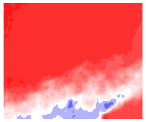
Figure 2. (a) Instantaneous contours of streamwise velocity and (b) contours of γ in the streamwise–wall-normal measurement plane. (c) Instantaneous contours of the streamwise velocity and (d) contours of γ in the streamwise–spanwise plane located at y/δ 0 = 0.22. The detachment and endpoints of the instantaneous TSB are labelled in (a) as points D′ and E′, respectively.
The contours of the forward-flow probability, γ, in figure 2(b) show the intermittency of the TSB boundaries. Starting from an upstream location, γ gradually reduces with increasing x/c approximately until the TE. Along a near-wall line of y/c = 0.003, γ reaches a minimum value of γ = 0.06 at x/c = −0.02, which is just upstream of the TE. Between x/c = −0.02 and the TE, γ rapidly increases to γ = 1 over a short distance. Scrutiny of the instantaneous visualizations shows occasional forward flows in the small region between x/c = −0.02 and the TE. However, since γ reaches a negligible value of 0.06 at a small distance of 0.02c upstream of the TE, the TE can be assumed as a fixed corner of the TSB. Downstream of the TE along y/c = 0, γ remains equal to 1 due to the high-velocity flow of the pressure side crossing the wake centreline. In contrast, along the diagonal path that is indicated with a dashed line in figure 2(b), γ gradually increases from 0.1 to 0.99 over a distance of approximately 0.1c. The trailing region of the TSB is therefore highly intermittent as the back-flow region moves back and forth along the dashed line (also see supplementary movie 1). Overall, the results indicate that the TSB features an intermittent detachment on the airfoil surface, an intermittent back-flow region that extends diagonally into the wake region, and a point just upstream of the TE that is approximately fixed. This triangular-shaped TSB is different from the dome-shaped TSBs of Mohammed-Taifour & Weiss (Reference Mohammed-Taifour and Weiss2016), Le Floc'h et al. (Reference Le Floc'h, Weiss, Mohammed-Taifour and Dufresne2020) and Wu et al. (Reference Wu, Meneveau and Mittal2020) that consist of a single shear layer evolving near a wall. For this configuration, the breathing motion is defined as low-frequency variations of the TSB cross-sectional area in the streamwise–wall-normal plane.
An instantaneous streamwise velocity field from the streamwise–spanwise PIV plane is shown in figure 2(c). The TE is located at the most downstream location of this measurement plane at x/c = 0. The black line indicates the contour of U = 0 which separates the upstream forward flow from the downstream back-flow region and therefore outlines the TSB. This separation line is oriented in the spanwise direction, but it undulates due to the intermittency of the separation location. The undulating pattern of the separation line is attributed to its interaction with the low- and high-speed structures of the incoming TBL (Eich & Kähler Reference Eich and Kähler2020; Ma et al. Reference Ma, Gibeau and Ghaemi2020). The time instance shown in figure 2(c) also contains a relatively rare event in which the flow stays attached up to the TE at z/c > 0.13. There are also a few isolated back-flow regions within the forward-flow region and a few small pockets of forward flow within the separation bubble, as indicated within the figure. To demonstrate these features over time, a sequence of time-resolved velocity fields in the streamwise–spanwise plane is shown in supplementary movie 2.
To statistically investigate the intermittency of the TSB in the streamwise–wall-normal plane, we have plotted the contours of forward-flow probability which are shown in figure 2(d). The iso-contours of γ are mainly oriented in the spanwise direction as the forward-flow probability reduces with increasing x/c. A contour with a low γ of 0.1 is observed just upstream of the TE. It is also observed that the contours have a wavy pattern that undulates in the streamwise direction. The undulation is small relative to the chord length as the maximum oscillation of the γ = 0.99 contour is approximately 0.1c. The wavy pattern is due to the presence of three-dimensional (3-D) flow structures that are known as stall cells. These structures commonly form during flow separation on 2-D wings, and each stall cell consists of a saddle point and a pair of foci (Weihs & Katz Reference Weihs and Katz1983). Multiple stall cells and asymmetric patterns can form along the wingspan depending on the angle of attack, Reynolds number, airfoil shape and the aspect ratio of the wing (Dell'Orso, Tuna & Amitay Reference Dell'Orso, Tuna and Amitay2016; Dell'Orso & Amitay Reference Dell'Orso and Amitay2018; Wang & Ghaemi Reference Wang and Ghaemi2021). In addition to the stall cells, Wang & Ghaemi (Reference Wang and Ghaemi2021) observed that secondary structures are present at the two spanwise ends of the current wing configuration around z/c = ± 0.62, which may contribute to the asymmetry of the wavy pattern of the separation line with respect to the centreline of the wing (z/c = 0). However, due to the large span of the wing, these structures are far from the measurement domain and are not expected to affect the TSB dynamics.
Contours of normalized mean streamwise velocity, 〈U〉/U∞, in the streamwise–wall-normal plane are illustrated in figure 3(a). The solid line shows the contour of 〈U〉 = 0, which represents the boundary of the mean TSB. The most upstream point of 〈U〉 = 0 at x/c = −0.13 is the mean detachment point, as indicated by the letter D. The end of the mean TSB is specified by the letter E and is located at  $({x_E}/c,{y_E}/{\delta _0}) = (0.03,1.1)$. The mean length of the separation bubble, l, is defined as the distance between D and E, which is 0.16c. Similar to the instantaneous TSB, the mean TSB has a triangular shape with its three vertices at D, E and the TE. The TBL over the suction side of the airfoil detaches from the wall and forms the upper shear layer that extends along the DE line. The mean TSB is relatively shallow with an approximate height of 0.02c, which is attributed to the pre-stall angle of attack of the wing (Wang & Ghaemi Reference Wang and Ghaemi2021). As noted previously, the lower shear layer forms from the separation of the high-speed flow emerging from the pressure side of the airfoil. The upper and lower shear layers are labelled in figure 3(a).

Figure 3. (a) Contours of 〈U〉/U∞ in the streamwise–wall-normal plane revealing the triangular-shaped TSB. (b) Contours of 〈V〉/U∞ in the streamwise–wall-normal plane with an overlay of mean flow streamlines. (c) The variation of boundary layer thickness, momentum thickness and the pressure coefficient with streamwise distance. (d) Contours of 〈U〉/U∞ in the streamwise–spanwise plane. In (a) and (d), the black line shows the contour of 〈U〉 = 0. The detachment and endpoints of the time-averaged TSB are labelled in (a) as points D and E, respectively.
Figure 3(b) shows contours of the normalized wall-normal velocity, 〈V〉/U∞, and the mean flow streamlines in the streamwise–wall-normal plane. The free-stream flow upstream of the measurement domain has a small positive 〈V〉/U∞, mainly due to the downstream blockage caused by the TSB. The wall-normal component then increases with increasing x/c as the flow passes over the TSB. There is a small region of negative 〈V〉/U∞ within the TSB due to the downward motion of the recirculating vortex. A strong upward flow emerges from the pressure side of the airfoil into the wake region. This upward flow pushes the trailing section of the TSB in the positive y direction.
The variation of the boundary layer thickness, δ 95, and momentum thickness, θ, of the incoming TBL with respect to x/c is demonstrated using the left-side axis of figure 3(c). The streamwise extent of the reported δ 95 and θ in this figure is limited to the region where the TBL stays attached to the wall. Due to the wall-normal limit of the measurement domain, the boundary layer thickness has been obtained based on the y location where 〈U〉 = 0.95U∞, and the integration of the velocity profiles for calculating θ is also carried out up to the same location where 〈U〉 = 0.95U∞. Figure 3(a) shows that both δ 95 and θ gradually increase with respect to x/c until x/c = −0.22 where the change in δ 95 and θ suddenly increases. The sudden increase is attributed to the instantaneous presence of back flow (γ becoming smaller than 1) as can be seen in figure 2(b). The value of Reθ, which is calculated based on U∞ and θ at an upstream location of x/c = −0.35, is approximately 2800. This Reθ is larger than the Reθ of 490 considered in the DNS of Wu et al. (Reference Wu, Meneveau and Mittal2020) but smaller than the Reθ of 5000 considered by Weiss et al. (Reference Weiss, Mohammed-Taifour and Schwaab2015). The friction Reynolds number, Reτ, defined using friction velocity and boundary layer thickness, is approximately equal to 900. This value is estimated here using the  $R{e_\tau } = 1.13 \times Re_\theta ^{0.843}$ equation proposed by Schlatter & Örlü (Reference Schlatter and Örlü2010).
The right-side axis of figure 3(a) also shows the variation of the static pressure coefficient, CP, measured along the midspan of the wing from x/c = −0.31 to −0.08. The results reveal the presence of an APG with a larger increase in CP upstream of the TSB from x/c = −0.31 to approximately x/c = −0.2. This is followed by a slower increase in CP from x/c = −0.2 to −0.08, which overlaps with the mean TSB. The largest CP observed here is approximately half of the maximum CP reported in the experiments of Weiss et al. (Reference Weiss, Mohammed-Taifour and Schwaab2015) and Le Floc'h et al. (Reference Le Floc'h, Weiss, Mohammed-Taifour and Dufresne2020) and the simulations of Wu et al. (Reference Wu, Meneveau and Mittal2020).
The contours of 〈U〉/U∞ in the streamwise–spanwise plane are shown in figure 3(d). The separation point along the midspan (z/c = 0) is at x/c = −0.15, which is slightly downstream of the point D detected in figure 3(a). This small shift is because the wall-parallel measurement plane is at approximately y/δ 0 = 0.22 while the first data point in the streamwise–wall-normal PIV plane is at y/δ 0 = 0.17. The contours of mean velocity exhibit a wavy separation line, which is similar to the pattern of the γ contours in figure 2(d). As was discussed previously, the wavy pattern and its asymmetry are associated with stall cells and secondary structures formed along the wingspan (Wang & Ghaemi Reference Wang and Ghaemi2021).
The Reynolds stresses are calculated with respect to a curvilinear coordinate system with xc and yc axes based on a streamline that approximately follows the loci of maximum spanwise vorticity along the upper shear layer. The path of the curvilinear coordinate system is shown with a dashed line in figure 4(a). The xc axis remains tangent to the line while its positive direction is in the flow direction. The yc axis is perpendicular to xc and is positive in the counterclockwise direction with respect to the positive xc axis. The parameters calculated in this curvilinear coordinate system are shown with subscript c. The conversion of the Reynolds stresses from the fixed x−y coordinate system to this curvilinear coordinate system is performed following Wu & Piomelli (Reference Wu and Piomelli2018) and Fang & Tachie (Reference Fang and Tachie2020). Inspection of the Reynolds stresses in the x–y and xc–yc coordinates shows that the magnitudes are different while the spatial pattern of the Reynolds stresses remains similar.

Figure 4. The contours of (a)  ${\langle {u^2}\rangle _c}$, (b) ${\langle {v^2}\rangle _c}$ and (c) ${\langle uv\rangle _c}$, normalized by $U_\infty ^2$. The velocity components are computed in the curvilinear xc–yc coordinate system shown in (a). The contour line shows the boundary of the mean TSB based on $\langle U\rangle = 0$.
The normalized contours of streamwise Reynolds stress,  ${\langle {u^2}\rangle _c}$, in figure 4(a) exhibit two high-intensity zones that correspond to the upper and lower shear layers. The upper shear layer is wider and has a slightly higher peak intensity. Along the upper shear layer, the magnitude of ${\langle {u^2}\rangle _c}$ initially rises with increasing x/c and reaches its maximum downstream of the TE at approximately x/c = 0.1. Farther downstream, ${\langle {u^2}\rangle _c}$ gradually decreases as the upper shear layer progresses into the wake region. This trend is similar to the distribution of streamwise Reynolds stress shown in the APG-induced TSBs of Mohammed-Taifour & Weiss (Reference Mohammed-Taifour and Weiss2016), Le Floc'h et al. (Reference Le Floc'h, Weiss, Mohammed-Taifour and Dufresne2020) and Mohammed-Taifour & Weiss (Reference Mohammed-Taifour and Weiss2021). In these investigations, the streamwise Reynolds stresses demonstrated a single peak within the shear layer, which was close to the detachment point. The DNS of Wu et al. (Reference Wu, Meneveau and Mittal2020) also shows a single peak near the detachment location when they forced the shear layer to reattach by imposing an FPG. In contrast, when Wu et al. (Reference Wu, Meneveau and Mittal2020) did not apply a FPG, a strong second peak appeared close to the reattachment region. The shear layer in the DNS of Na & Moin (Reference Na and Moin1998) also shows two local peaks of streamwise Reynolds stress; the first one was close to the detachment point and the second one was in the downstream part of the TSB. In both Wu et al. (Reference Wu, Meneveau and Mittal2020) and Na & Moin (Reference Na and Moin1998), the second peak potentially forms due to stronger interactions between the shear-layer vortices and the wall during the gradual reattachment process. Such an interaction is not present for the TE separation of the current investigation as the shear layer departs from the airfoil surface and oscillates freely in the wake region. In addition, the current TSB has a strong lower shear layer with two peaks: a small intense region of ${\langle {u^2}\rangle _c}$ near the TE and a second peak farther downstream at approximately x/c = 0.05.
Normalized contours of  ${\langle {v^2}\rangle _c}$ are shown in figure 4(b), where the upper shear layer has a significantly weaker magnitude relative to the lower shear layer. Our analysis indicates that the difference is not due to the alignment of the curvilinear coordinate system with the upper shear, as the magnitude of ${\langle {v^2}\rangle _c}$ in the lower shear layer is greater than that of the upper shear layer even if the curvilinear coordinate system is aligned with the trajectory of the lower shear. The greater ${\langle {v^2}\rangle _c}$ of the lower shear layer is associated with the greater velocity gradient across the lower shear layer, as can be seen in figure 3(a). This results in the roll-up of stronger spanwise vortices. The intense wall-normal velocity fluctuations of the lower shear also result in stronger Reynolds shear stresses as shown in figure 4(c). The high 〈 $uv$〉c region of the lower shear layer is narrower and more concentrated relative to the upper shear layer. The normalized 〈 $uv$〉c in the lower shear layer reaches 0.012, while it only reaches −0.003 along the upper shear layer. As expected, both shear layers contribute to the production of turbulence; the opposite 〈 $uv$〉c signs cancel with the opposite signs of mean velocity gradient, d〈U〉c/dyc, for the two shear layers. The Reynolds stress distributions also show that the two shear layers do not fully merge within the measurement domain as they maintain separate regions of strong Reynolds stresses. However, the lower shear layer dominates the upper shear layer in terms of wall-normal and shear Reynolds stresses. This contrasts with the previous investigations of TSBs on flat plates in which the Reynolds stresses are concentrated in the single shear layer that forms above the TSB.
The normalized intensity of Reynolds stresses in the current TSB can be compared with those of turbulent plane mixing layers. The  ${\langle {u^2}\rangle _c}/U_\infty ^2$ peak of the upper and lower shear layers in figure 4(a) reach 0.02, which is similar to the 0.03 peak observed in Forliti, Tang & Strykowski (Reference Forliti, Tang and Strykowski2005) and Loucks & Wallace (Reference Loucks and Wallace2012) for plane shear layers. In contrast, only the ${\langle {v^2}\rangle _c}/U_\infty ^2$ peak of the lower shear layer is similar to the $\langle {v^2}\rangle /U_\infty ^2$ peak of 0.02 observed in Forliti et al. (Reference Forliti, Tang and Strykowski2005) and Loucks & Wallace (Reference Loucks and Wallace2012). A similar observation is made for Reynolds shear stress. The ${\langle uv\rangle _c}/U_\infty ^2$ peak of the lower shear layer in figure 4(c) is similar to the 0.01 peak reported in Loucks & Wallace (Reference Loucks and Wallace2012), while the peak value of the upper shear layer is an order of magnitude smaller. Therefore, the intensity of Reynolds stresses in lower shear layer of the TSB resembles those of plane shear layers, while the upper shear layer demonstrates smaller values of wall-normal and shear Reynolds stresses.
To characterize the thickness of the shear layers, the distribution of the normalized mean spanwise vorticity, 〈ωz〉l/U∞, is shown in figure 5(a). The trajectories of the maximum vorticity along each shear layer are also plotted as black dashed lines. The upper shear layer has a wide region of negative 〈ωz〉, while the lower shear layer has a thin zone of positive 〈ωz〉. For both shear layers, the 〈ωz〉 magnitude gradually reduces in the flow direction. The shear-layer thickness δ is estimated as the wall-normal extent of the region where  $|\langle {\omega _z}\rangle /{\langle {\omega _z}\rangle _{peak}}|> 1/e$. Here, ${\langle {\omega _z}\rangle _{peak}}$ is the local maximum vorticity and e is the exponential constant. The estimated δ has been normalized using l and is shown in figure 5(b). The results show that the thickness of the upper shear layer initially increases with increasing x/c until the TE, at which point the thickness of the layer reduces, potentially due to the appearance of the lower shear layer. Within 0.16 < x/c < 0.22, the thickness of the upper shear stays relatively constant at δ/l ≈ 0.24, and then reduces again close to the end of the measurement domain. In contrast, the thickness of the lower shear layer continuously increases within the measurement domain, and even surpasses the thickness of the upper shear layer at x/c = 0.24.

Figure 5. (a) Contour of  $\langle {\omega _z}\rangle$ normalized by U∞/l. The black dashed lines follow the location of peak vorticity, ${\langle {\omega _z}\rangle _{peak}}$, along the upper and lower shear layers. (b) The variation of vorticity thickness, δ, for the upper and lower shear layers with respect to x/c.
4. Unsteady motions
To characterize the frequency and energy of flow unsteadiness, the pre-multiplied power spectral density (PSD) of streamwise velocity fluctuations (u) along y/δ 0 = 1.0 is presented in figure 6(a). The PSD was calculated by dividing each of the 15 datasets into 3 segments with 50 % overlap. This resulted in 45 periodograms, each 44l/U∞ long, which were normalized using the square of the free-stream velocity and then multiplied by f. Note again that Stl is defined as fl/U∞ where the length scale, l, is equal to the length of the upper edge of the mean TSB (0.16c). The pre-multiplied PSD contours show strong unsteadiness in the upstream TBL, inside the TSB, and across the lower shear layer as labelled in figure 6(a). In the upstream TBL, the energetic flow motions have a high Stl of approximately 4, which gradually reduces to 0.1 with increasing x/c. The reduction in the Stl of the TBL fluctuations is attributed to the effect of the APG on the low- and high-speed structures (Skote & Henningson Reference Skote and Henningson2002; Lee & Sung Reference Lee and Sung2009; Eich & Kähler Reference Eich and Kähler2020).

Figure 6. Contours of the pre-multiplied PSD of u along (a) y/δ 0 = 1.0, (b) the upper shear layer and (c) the lower shear layer. Note that Stl = 4.2 × Stδ.
A zone of energetic motions with small Stl is observed in the range −0.15 < x/c < +0.02, which overlaps with the streamwise location of the TSB where forward-flow probability is relatively small. According to figure 2(b), γ varies from 0.5 to 0.1 within this high-energy zone. The maximum energy of these motions is centred at Stl of 0.06 while some of the fluctuations occur at smaller Stl of 0.03. These frequencies are similar to the Stl = 0.03 reported for the breathing motion by Weiss et al. (Reference Weiss, Mohammed-Taifour and Schwaab2015). The current investigation indicates that energetic velocity fluctuations with small Stl = 0.03 are present in an APG-induced TSB. The observation of low Stl breathing motion by Weiss et al. (Reference Weiss, Mohammed-Taifour and Schwaab2015) was based on wall-pressure measurements, which can be the result of flow motions throughout the whole flow field. The PSD of streamwise velocity by Wu et al. (Reference Wu, Meneveau and Mittal2020) also does not indicate the present of velocity fluctuations at such a low frequency, potentially because their spectrum was limited to Stl > 0.2 and the streamwise velocity was averaged over the spanwise direction. We will further investigate these low Stl motions to characterize their spatial structure and indicate whether they are related to the breathing motion.
Figure 6(a) also reveals a zone of energetic flow motions with Stl varying from 0.1 to 10 at x/c = 0.04. This location is downstream of the TE and corresponds to the intersection of the lower shear layer with y/δ 0 = 1.0. The wide Stl range at this location is a result of the spatial displacement of the shear layer as seen by a fixed grid point of the PIV FOV. As the shear layer oscillates in space, the turbulent shear layer and the free-stream flow intermittently occupy the PIV grid point, and therefore the pre-multiplied PSD spreads over a broad range of Stl from 0.1 to 10. To address this issue, the pre-multiplied PSDs of u have been computed along the upper and lower shear layers and are presented in figures 6(b) and 6(c), respectively. The trajectories along which the pre-multiplied PSDs were computed are the same as those shown with dashed lines in figure 5(a). Moreover, to allow for comparison of the present results with previous characterizations of shear layers, the frequency was normalized as Stδ = fδ/U∞. Here, δ is the thickness of the upper shear layer at x/c = 0.2, which is equal to 0.24l based on figure 5. The contours of figure 6(b) show that the energy of the fluctuations increases with increasing x/c along the upper shear layer. The strongest oscillations are observed close to the TE, at approximately x/c = 0.1, with a Stδ of 0.05 to 0.2 (equivalent to Stl of 0.2 to 0.8). With increasing x/c, the oscillations converge to Stδ of 0.15 (Stl of 0.4). The results for the lower shear layer in figure 6(c) show energetic motions at Stδ of 0.1 to 0.2 (Stl of 0.4 to 0.8). The value of Stδ of the flow oscillations along both shear layers is similar to the Strouhal number of vortex shedding reported in previous experimental investigations (Maull & Young Reference Maull and Young1973; Sigurdson Reference Sigurdson1995) and the Strouhal number of the most amplified frequencies predicted by the linear stability theory for shear layers (Monkewitz & Huerre Reference Monkewitz and Huerre1982). Therefore, both shear layers are subject to Kelvin–Helmholtz instabilities, which result in the roll-up of the shear layer and vortex shedding.
5. Temporal and spatial scales
The temporal evolution of spanwise profiles of u/U∞ is shown in figure 7 for three x/c locations of −0.25 (within the upstream TBL), −0.15 (close to the mean separation point) and −0.05 (within the TSB). The vertical axis of the figure is the spanwise axis of the flow, z/c, while the horizontal axis is the normalized time, t/T. Here, T is a time scale defined as l/U∞. All the data correspond to y/δ 0 = 0.22, which is the wall-normal location of the streamwise–spanwise PIV plane. The flow pattern at x/c = −0.25 includes streamwise regions of low- and high-speed flows. The structures meander in the spanwise direction and they have a spanwise spacing of approximately 0.04c, which is equal to 1.1δ 95 (based on the local thickness of the TBL at x/c = −0.25). This spanwise spacing is similar to the spanwise spacing of ~1δ 95 reported by Ganapathisubramani et al. (Reference Ganapathisubramani, Hutchins, Hambleton, Longmire and Marusic2005) for large-scale motions at y/δ 95 = 0.5 in a TBL with Reτ = 1100. Therefore, the wall-normal location of the measurement plane (y/δ 0 = 0.22) and the spanwise spacing of the structures seen at x/c = −0.25 suggest that the pattern corresponds to the large-scale motions (LSM) and the very-large-scale motions of the outer layer (Balakumar & Adrian Reference Balakumar and Adrian2007; Hutchins & Marusic Reference Hutchins and Marusic2007).

Figure 7. Instantaneous visualization of spanwise profiles of u/U∞ as they evolve in time at three streamwise locations of x/c = −0.25, −0.15 and −0.05.
At x/c = −0.15 and −0.05 in figure 7, which correspond to upstream of the mean TSB and within the TSB, the flow pattern consists of large zones of positive and negative velocity fluctuations. These zones have a large spatio-temporal coherence; they are several times wider than those observed at x/c = −0.25 and they appear longer along the time axis. The latter suggests that they have a slower advection velocity or a longer streamwise length. The large zones at x/c = −0.15 and −0.05 resemble the highly elongated streamwise structures that Wu et al. (Reference Wu, Meneveau and Mittal2020) observed in the low-frequency modes of their DMD analysis. They attributed the structures to Görtler vortices generated by the curvature of the streamlines as the flow passes over the separated region. The zones also resemble the large Görtler structures shown by You, Buchta & Zaki (Reference You, Buchta and Zaki2021) in the DNS of a TBL over a concave wall.
To further investigate the spatial and temporal scales of the structures, the fluctuating streamwise velocity along the x-axis is plotted versus time in figure 8. The data correspond to a streamwise profile of u/U∞ at the midspan of the wing (z/c = 0) and are extracted from the streamwise–spanwise PIV plane. To illustrate structures with both short and long temporal scales, figure 8(a) shows a shorter duration of 20T while figure 8(b) shows a longer duration of 98T. The instantaneous separation line, which is the location of U = 0, is also shown with a solid black line. A pattern of inclined low- and high-speed structures is seen upstream of the separation region at approximately x/c < −0.2 within figure 8(a). Each stripe shows the advection of a low- or a high-velocity structure in the x–t domain. Since the large-scale structures of TBLs meander in the z-direction, the length of the stripes visible in figure 8 does not reveal their full streamwise extent or lifetime. However, the inclination/slope of each stripe, i.e. dx/dt of the lines tangent to the stripes, indicates their advection speed. For example, the slope of the dashed line seen at t/T ≈ 2 in figure 8(a) indicates that the high-speed structure tangent to this line moves downstream at a speed of 0.4U∞. As the structures approach the separation line, they become wider and their slopes reduce, thus indicating a slower advection speed. The widening is pronounced for the high-speed structures in the region immediately upstream of the instantaneous separation line. The slower advection speed is seen by the gradual departure of the high-speed structure at t/T ≈ 2 from its corresponding dashed line. In addition, the horizontal spacing between the adjacent structures along the t/T axis represents their frequency. The closely packed structures at x/c < −0.2 appear to alternate in periods as short as 0.5T, which is equivalent to Stl = 2. Therefore, the high-frequency oscillations that were observed within the upstream TBL of figure 6(a) are indeed associated with the TBL structures.

Figure 8. The temporal evolution of streamwise profiles of u/U∞ over (a) a short duration of 20T and (b) a longer duration of 98T. The data correspond to the midspan of the wing (z/c = 0) from the streamwise–spanwise PIV plane at y/δ 0 = 0.22.
Once the flow reaches the separation region at approximately x/c = −0.2 of figure 8(a), the large zones of positive and negative velocity fluctuation emerge. These large zones correspond to the motions within the TSB (under the separated shear layer) along the y/δ 0 = 0.22 plane. They extend along the time axis and occasionally appear to linger at a fixed location due to their lower advection speeds. As seen from the negative slope of the dashed line drawn at t/T ≈ 7 in figure 8(a), some of the zones with negative u appear to slowly advect in the upstream direction, i.e. a back-flow motion within the TSB. The positive and negative zones of the TSB alternate slowly over long periods reaching up to 50T as seen in the longer sequence of figure 8(b). This duration is equivalent to Stl = 0.02, which is similar to the low Stl motions observed within the TSB in figure 6(a). It is also observed that the separation line in figure 8(b) closely follows the pattern of these large zones. At t/T ≈ 50 a negative zone results in the separation front moving in the upstream direction, while at t/T ≈ 90 a positive zone results in the separation front moving downstream.
The present results indicate that the TSB is formed from large zones featuring positive and negative streamwise velocity fluctuations. When compared with the low- and high-speed structures of the upstream TBL, these TSB structures are several times wider and their time scale is approximately two orders of magnitude greater. These low- and high-speed zones result in the energetic, low-frequency region labelled as TSB in the pre-multiplied PSD of figure 6(a).
In figure 9, the spatial and temporal scales of the turbulent structures are quantified using results extracted from two-point correlations of the streamwise velocity fluctuations. The reference point for these correlations was placed at a spatial location of (x 0, y 0, z 0) and at an arbitrary reference time, t 0. The correlation coefficient, Ruu, was calculated according to
 \begin{equation}{R_{uu}}(\Delta x,\Delta y,\Delta z,\Delta t) = \; \frac{{\langle {u_{({x_0},{y_0},{z_0},{t_0})}}{u_{({x_0} + \Delta x,{y_0} + \Delta {y_0},{z_0} + \Delta z,{t_0} + \Delta t)}}\rangle }}{{\sqrt {\langle u_{({x_0},{y_0},{z_0},{t_0})}^2\rangle } \; \sqrt {\langle u_{({x_0} + \Delta x,{y_0} + \Delta {y_0},{z_0} + \Delta z,{t_0} + \Delta t)}^2\rangle } }}.\end{equation}
In this equation, Δx, Δy, Δz and Δt indicate the spatial and temporal offsets of the traversed data point with respect to the reference point. Each offset was applied separately, e.g. when Δx was varied, Δy, Δz and Δt were kept constant at zero. The streamwise location of the reference point was varied within −0.35 < x 0/c < 0 when Δy, Δz and Δt were applied. A smaller streamwise extent of −0.28 < x 0/c < −0.11 was used while varying Δx to ensure that x 0 ± Δx remains within the measurement domain. To improve the statistical convergence, the correlation functions were averaged along the spanwise direction of the measurement domain where possible. Once the correlation functions were obtained, the length and time scales of the structures were determined as the point at which Ruu = e −1. The estimated streamwise, wall-normal, and spanwise length scales are denoted by lx, ly and lz, and the temporal scale is denoted by lt. The wall-normal scale, ly, was obtained from the streamwise–wall-normal PIV plane, while lx, lz and lt were obtained from the streamwise–spanwise PIV plane. For consistency, the wall-normal location of the reference points in the streamwise–wall-normal PIV plane was selected as y 0 = 0.22δ 0, which is the same location as the streamwise–spanwise plane.

Figure 9. The (a) spatial and (b) temporal scales of the motions estimated based on two-point correlations of the streamwise velocity fluctuations. The spatial scales, li, are normalized using δ 0, and the temporal scale is normalized using T, defined as l/U∞.
In figure 9(a), all length scales can be seen to increase with increasing x 0/c. The largest rate of increase in lx is seen at approximately x 0/c = −0.24, which overlaps with the start of the intermittency boundary of the TSB (the γ = 0.99 contour, figure 2b). Farther downstream at x 0/c = −0.1, the rate of increase in lx is small as its curve appears to approach an asymptotic value. This asymptotic value is approximately twice the value of lx at x 0/c = −0.28, which suggests that the structures become longer by a factor of 2. However, it is important to note that the estimated length scale does not consider the spanwise meandering of the associated structures and therefore lx does not represent their true length. A similar trend is also observed for lz, which indicates that the length scale increases by a factor of three with increasing x 0/c. For ly, we observe a sharp reduction just upstream of the TE at x 0/c = −0.02. Inspection of the instantaneous velocity fields shows that this reduction is due to the frequent presence of forward flow in this region, which is indicated by the rapid increase in γ just upstream of the TE shown in figure 2(b). Overall, the larger length scales of the structures within the TSB are consistent with the visualizations of figures 7 and 8. The estimated time scale, lt, in figure 9(b) also increases with increasing x 0/c until approximately x 0/c = −0.15, where lt can be seen to reach a maximum value. The large time scale at this location agrees with the low Stl motions observed within the TSB in figure 6(a). Farther downstream, lt decreases and reaches a smaller value of approximately 2.7. This analysis using two-point correlations statistically confirms the TSB zones have a greater spatial and temporal scale with respect to the largest structures of the upstream TBL.
To identify the source of the large low- and high-speed zones of the TSB, we evaluate the formation of Görtler vortices (Görtler Reference Görtler1954) following the procedure applied by Wu et al. (Reference Wu, Meneveau and Mittal2020). The Görtler number, GT, is calculated using the local radius of curvature of several streamlines that closely pass over the mean TSB. For calculating GT, an effective eddy viscosity is also calculated using the streamwise–wall-normal component of Reynolds shear stress. The results show that GT value reaches the 0.3 criterion that is required for the formation of Görtler vortices at approximately x/c = −0.22 and then rapidly increases beyond this limit until the mean separation point is reached. In addition, δ 95/R also serves as a criterion for predicting the presence of Görtler vortices (Floryan Reference Floryan1991). The δ 95/R value reaches the proposed limit of 0.01 at approximately x/c = −0.25 and then rapidly increases beyond this limit to values of the order of 0.1 at x/c = −0.1. Therefore, both GT and δ 95/R suggest that Görtler vortices can form upstream of the current TSB. We conjecture that the large low- and high-speed zones that are observed at x/c = −0.15 and −0.05 of figure 7 and the downstream region of figure 8 correspond to the footprint of the Görtler vortices.
The Ruu contours for simultaneous streamwise and wall-normal shifts (Δx and Δy) are shown in figure 10. Five reference locations at y 0/δ 0 = 0.22 and x 0/c = −0.3, −0.25, −0.2, −0.15 and −0.05 were selected from the streamwise–wall-normal PIV plane. The centrelines of the upper and lower shear layers (from figure 5a) are also shown in figure 10 using dashed lines. As expected from figure 9, the correlation function becomes larger in the streamwise and wall-normal directions with increasing x 0/c. The correlation patterns are also slightly inclined in the position x direction. Interestingly, the last correlation function, which features a reference at (x 0, y 0) = (−0.05c, 0.22δ 0), shows a double-peak pattern with the second peak located between the upper and lower shear layer at (x/c, y/δ 0) = (0.02, 2.0). This correlation pattern indicates that the large positive and negative zones of the TSB correlate with the velocity fluctuations generated between the two shear layers by the vortex shedding process.

Figure 10. The correlation functions for five reference points located at y 0/δ 0 = 0.22 and x 0/c = −0.3, −0.25, −0.2, −0.15 and −0.05. The most downstream correlation function shows a double-peak pattern.
6. Energetic motions
In this section, SPOD of the velocity fields, based on the algorithm described by Towne, Schmidt & Colonius (Reference Towne, Schmidt and Colonius2018), is used to identify the frequency and spatial pattern of the energetic motions. This algorithm decomposes the Fourier transform of the velocity fields into spatial modes, Φi (x, f) and expansion coefficients, ai (f). Here, the index i denotes the mode number, and x is a vector indicating the spatial location.
Figure 11 shows the energy associated with the first three SPOD modes. These SPOD modes have been obtained from both components of the streamwise–wall-normal velocity fields using 15 planar PIV datasets. Each dataset is approximately 1.21 s long and is divided into three blocks with 50 % overlap for SPOD calculations. As expected, the first mode captures the highest percentage of the energy, while the second and third modes have a negligible energy across the frequency spectrum. The separation in the energy of the first and second mode is relatively large at Stl < 0.1, which indicates a low-rank behaviour (Schmidt et al. Reference Schmidt, Towne, Rigas, Colonius and Brès2018). The first mode shows the highest energy at the lowest resolved Stl of 0.02, which is similar to the Stl of breathing motion reported by Weiss et al. (Reference Weiss, Mohammed-Taifour and Schwaab2015) and Mohammed-Taifour & Weiss (Reference Mohammed-Taifour and Weiss2016). The first mode also exhibits smaller local peaks at approximately Stl = 0.16 and 0.72. The Stl of these peaks is close to the vortex shedding frequency, which is approximately at Stl = 0.2 to 0.8 according to figure 6.

Figure 11. The energy spectra of the first three SPOD modes calculated from the streamwise–wall-normal velocity fields.
The spatial patterns of the first SPOD mode at Stl = 0.02, 0.16 and 0.72 from the streamwise–wall-normal plane are shown in figure 12. In addition, a reduced-order model (ROM) of the flow field, U ROM, has been constructed using the mean velocity field and the selected mode following
 \begin{equation}{U_{ROM,i}} = U + {\varPhi _{i(x,{f_0})}}\,{\textrm{e}^{2{\rm \pi} i{f_0}t}}.\end{equation}
Here, t is time and f 0 is the frequency of the selected SPOD mode used for reconstructing the ROM. The forward-flow probability, γ, for the ROMs constructed from each spatial mode at the selected f 0 was then computed and is shown using the contour lines in figure 12. The spatial pattern of the first mode at Stl of 0.02 consists of a large, inclined structure that is approximately aligned with the upper shear layer. The γ contours of this first mode show that it is associated with the large-scale expansion and contraction of the TSB. These contours are also similar to those of the forward-flow probability previously observed in figure 2(b), which shows that this spatial pattern captures the dominant large-scale unsteadiness within the streamwise–wall-normal plane. The small Stl of this SPOD mode and the fact that this mode is the main contributor to the intermittency of the TSB suggest that it is associated with the breathing motion of the TSB. As noted previously, in the context of TE separation, the breathing motion is defined as low-frequency variations of the TSB cross-section. This SPOD mode is consistent with the proper orthogonal decomposition (POD) analysis of Mohammed-Taifour & Weiss (Reference Mohammed-Taifour and Weiss2016), which showed that the first POD mode in the streamwise–wall-normal plane is associated with the breathing motion. The second and third spatial patterns at Stl = 0.16 and 0.72 in figure 12 feature smaller structures that develop along the shear layers. The alternating spatial patterns, and their large Stl suggest that they capture the vortex shedding process of the shear layers. The intermittency contours in figure 12 indicate that the spatial pattern at Stl of 0.16 produce a considerable expansion/contraction of the TSB near the TE, while the spatial pattern at Stl of 0.72 does not result in a significant expansion or contraction of the TSB.

Figure 12. The spatial structures of the first SPOD mode from the streamwise–wall-normal plane at Stl = 0.02, 0.16 and 0.72. The contour lines represent the forward-flow probability obtained from the ROM following (6.1).
The three most energetic SPOD modes obtained using u and w from 10 datasets of the streamwise–spanwise PIV are shown in figure 13. Each dataset is approximately 1.35 seconds and is divided into three blocks with 50 % overlap (30 blocks in total). For all three modes, the low-frequency oscillations have a higher energy, with the maximum energy seen at the smallest Stl of 0.02. The energy of the modes quickly reduces with increasing Stl as most of the energy is at 0.02 < Stl < 0.1. In contrast to the SPOD modes of the streamwise–wall-normal velocity fields, there is no secondary peak at higher Stl. The small Stl of the energetic range frequency band suggests that the spatial modes do not attribute to LSM of the incoming TBL with 0.1 < Stl < 5, or the vortex shedding process with Stl = 0.4.

Figure 13. The energy spectra of the first three SPOD modes obtained from the streamwise–spanwise velocity fields.
The spatial patterns of the first SPOD mode at four Stl values of 0.02, 0.04, 0.06 and 0.08 are shown in figure 14. The forward-flow probability from the associated ROMs is also shown using contour lines. At Stl = 0.02 and 0.04, a single large-scale structure results in large expansion/contraction of the separation front. The forward-flow probability contours at these Stl values show large advancement/recession of the back-flow region. The spatial patterns at higher Stl of 0.04 and 0.06 consist of smaller alternating structures. However, their forward-flow probability contours still show considerable advancing and receding motions of the back-flow region. Therefore, the lead SPOD mode at the energetic frequencies with Stl < 0.1 captures large-scale back-and-forth motions of the separation front.

Figure 14. The spatial structures of the first SPOD mode of the streamwise–spanwise PIV plane at Stl = 0.02, 0.04, 0.06 and 0.08. The contour lines represent the forward-flow probability obtained from the ROM following (6.1).
7. The breathing motion
The breathing motion of the TSB is investigated in figure 15(a) using the pre-multiplied PSD of the instantaneous back-flow area, A, computed using the streamwise–wall-normal cross-section of the TSB. The figure also shows the pre-multiplied PSD of the streamwise location of the detachment point (xD ′), the streamwise location of the endpoint (xE ′) and the wall-normal location of the midpoint (yM ′). The coordinates of points D′, E′ and M′ are also obtained from the instantaneous streamwise–wall-normal PIV plane. The streamwise location of M′ is fixed at  ${x_{M^{\prime }}} = {\textstyle{1 \over 2}} \times ({x_{D}} + {x_{E}})$, which is the midpoint between the detachment and endpoints of the mean TSB, while its wall-normal location (yM ′) is detected from the instantaneous boundary of the TSB. Here, M′ is investigated to characterize the flapping motion, i.e. the wall-normal motion of the shear layer. Before calculating the PSDs, the mean value of each variable was subtracted and then it was normalized using its standard deviation, σ. As a result, the area under each curve in figure 15 is equal to one. Similar to the procedure applied for obtaining figure 6, the PSDs were calculated using 45 periodograms (each of the 15 datasets were divided into 3 segments with 50 % overlap).

Figure 15. (a) Pre-multiplied PSD of the fluctuations in A, xD ′, xE ′ and yM ′. (b) The coherence functions between A and the three TSB coordinates xD ′, xE ′ and yM ′. (c) The coherence between xD ′, xE ′ and yM ′.
The pre-multiplied PSD of A shows a large peak at approximately Stl = 0.05. The peak indicates expansions and contractions of the TSB area at low Stl, which is attributed to the breathing motion. The pre-multiplied PSD of A rapidly decreases at higher Stl and therefore the energetic expansions and contractions of the TSB area are limited to Stl < 0.1. The pre-multiplied PSD of xD ′ shows a broader range of energetic fluctuations with a peak approximately at Stl = 0.1. The broader energy distribution in the pre-multiplied PSD of xD ′ is attributed to the superposition of the small- and large-scale motion of the separation front seen in the spatial pattern of the SPOD modes of figure 14. The pre-multiplied PSD of xE ′ also has a broad energy distribution while it exhibits a higher energy at frequencies within the Stl = 0.1 to 0.3 range. The latter is slightly smaller than the vortex shedding Stl (from 0.2 to 0.8 based on figure 6). The discrepancy is associated with the interaction of the two shear layers, making the larger displacements of the endpoint to occur at the lower frequencies. The pre-multiplied PSD of yM ′ is similar to that of A with most of the energy at lower frequencies. The peak value is also at approximately Stl = 0.05 which is similar to the Stl of the breathing motion. This observation suggests that the expansions and contractions of the TSB at Stl = 0.05 should correlate with the flapping motion of the shear layer.
To further substantiate the above observations, the correlation between A and xD ′, xE ′ and yM ′ is quantified using the coherence functions shown in figure 15(b). The results show that the coherence function of A and xD ′ is relatively small across the investigated spectrum. This shows that the breathing motion does not strongly correlate with the motions of the detachment point. In contrast, the coherence of A and yM ′, and the coherence of A and xE ′, are large in the low-frequency range of Stl < 0.1. Therefore, the breathing motion correlates with both the flapping motion of the shear layer and the streamwise displacements of the TSB endpoint. The correlation between A and yM ′ was suggested based on figure 15(a) as both signals had high energy and similar pre-multiplied PSD shapes at Stl < 0.1. However, the correlation of A and xE ′ was not expected from figure 15(a) since the pre-multiplied PSD of xE ′ did not exhibit large energy at Stl < 0.1. Figure 15(b) also shows that coherence between A and yM rapidly declines with increasing Stl, while A and xE ′ remain relatively correlated at higher frequencies. The coherence function of A and xE ′ has a local peak at Stl of approximately 0.2, which overlaps with the peak energy observed in the pre-multiplied PSD of xE ′ of figure 15(a). In summary, the results show that the breathing motion (low-frequency expansion and contraction of the TSB cross-section in the streamwise–wall-normal plane) correlates with the shear-layer flapping and the displacements of the TSB endpoint.
The coherence functions between xD ′, yM ′ and xE ′ displacements are also investigated in figure 15(c). The results show that the detachment point, xD ′, does not correlate with the shear-layer flapping, yM ′, and the TSB endpoint, xE ′. This agrees with the previous observations that indicated the displacement of the detachment point are derived by the fluctuations of the upcoming TBL (Eich & Kähler Reference Eich and Kähler2020; Ma et al. Reference Ma, Gibeau and Ghaemi2020). Figure 15(c) also indicates that flapping motion of the shear layer correlates with the streamwise displacements of the endpoint at the low-frequency range of the spectrum.
The results showed that the large-scale expansion and contraction of the TSB area in the streamwise–wall-normal plane are mainly due to the oscillation of the endpoint and the wall-normal flapping of the TSB midpoint. In contrast, the motion of the detachment point has a smaller effect. However, the expansion and contraction of the TSB mainly occur at Stl = 0.05, which is smaller than the frequency of energetic motions of the detachment point at Stl = 0.1 to 0.3 (figure 15) or the vortex shedding frequency at Stl = 0.2 to 0.8 (figure 6). This discrepancy is associated with the spatial-averaging effect of the TSB. The mechanism is shown in figure 16 by plotting the pre-multiplied PSD of pointwise and spatially averaged streamwise velocity fluctuations along the shear layers. The pre-multiplied PSD of u at (x, y) = (0, 3.3δ 0) corresponds to a single point in the upper shear layer, above the TE. As it is observed, the energetic flow motions are at 0.2 < Stl < 1, which is consistent with the energetic motions seen in figure 6(b). The lines labelled as k = 0.5, 1 and 1.5 show the pre-multiplied PSD of streamwise velocity that is spatially averaged along the upper shear layer over a curvilinear trajectory that is centred at (x, y) = (0, 3.3δ 0) and extends in the upstream and downstream directions by 0.5l, 1l and 1.5l, respectively. Therefore, a spatially averaged velocity is first calculated as
 \begin{equation}{u_{avg}} = \int_{ - kl}^{ + kl} {u\,\textrm{d}\kern0.7pt{x_c}} ,\end{equation}
and then its pre-multiplied PSD is calculated. In this equation, xc is the curvilinear coordinate system defined in figure 4(a), and k is the kernel of the averaging line (k = 0.5, 1, and 1.5 in figure 16). The results show that by spatially averaging the velocity fluctuation the Stl of the energetic motions reduces to Stl = 0.2 for k = 0.5, and finally to a small Stl of 0.07 for k = 1.5. Therefore, figure 16 demonstrates that, although the vortex shedding process is at a higher Stl of 0.2 to 0.8, the ensemble effect of the velocity fluctuations along the shear layer is at a smaller Stl. This observation also suggests that the Stl of the breathing motion inversely scales with the TSB size; the larger the TSB, the greater is the effect of spatial averaging. This is consistent with the investigation of Le Floc'h et al. (Reference Le Floc'h, Weiss, Mohammed-Taifour and Dufresne2020) where three TSBs with small, medium and large sizes were investigated. Their measurements show that the larger TSB has the smallest breathing frequency, which is potentially due to spatial averaging of the velocity fluctuations over a longer shear layer.

Figure 16. Pre-multiplied PSD of streamwise velocity fluctuations at (x, y) = (0, 3.3δ 0) and pre-multiplied PSD of spatially averaged velocity according to (7.1).
8. Summary and conclusions
The TSB formed upstream of the TE of a 2-D wing was experimentally investigated. The wing was made from a NACA 4418 airfoil profile with a chord length, c, of 0.975 m and was set to an angle of attack of 9.7°. The Reynolds number based on c and the free-stream velocity was 720 000. The transition of the boundary layer to turbulence was forced using a trip wire placed 0.2c downstream of the wing leading edge. Measurements using time-resolved planar PIV were conducted in a large streamwise–wall-normal plane at the midspan of the wing using three synchronized high-speed cameras. The PIV measurements in a streamwise–spanwise plane that was parallel to and near the wing surface was also carried out using two synchronized high-speed cameras.
The PIV measurements showed that a TBL formed on the suction side of the wing. At 0.35c upstream of the TE, the Reynolds number of the TBL based on the free-stream velocity and the local momentum thickness was 2800, and the estimated friction Reynolds number, Reτ, was 900. Farther downstream, the TBL detached due to an APG. The mean detachment point of the TSB was 0.13c upstream of the TE. The TSB had a triangular shape skewed in the downstream direction. The size of the TSB was characterized using the length of its upper edge, l, which was equal to 0.16c. The three vertices of the triangular-shaped TSB consisted of (a) an intermittent detachment point, (b) an approximately fixed corner near the airfoil TE and (c) an intermittent endpoint in the wake region of the airfoil. The TSB featured two strong shear layers: an upper shear layer formed by the intermittent detachment of the suction-side TBL and a lower shear layer formed by the fixed detachment of the pressure-side boundary layer at the airfoil TE. The two shear layers generated zones of high Reynolds stress with peak intensities located downstream of the TE. The shear layers evolved in the wake region (free from the wall) and tended to gradually merge. The triangular shape of the TSB and the presence of the two shear layers differentiates this TSB from the dome-shaped TSB of previous investigations where a single TBL separates and reattaches over a flat plate. In the streamwise–spanwise plane, the TSB featured an undulating separation front.
Spectral analysis of the streamwise velocity fluctuations showed three energetic regions with different Strouhal numbers, Stl, defined as fl/U∞. The first region consisted of the energetic motions of the upstream TBL. The TBL fluctuations started with a large Stl = 4 which gradually reduced to Stl = 0.1 as the TBL approached the detachment point. These fluctuations were attributed to the LSM of the TBL, whose time scale gradually increased under the effect of the APG. The second energetic region was at the TSB location and featured motions at smaller Stl ranging from 0.03 to 0.08. The peak of these energetic motions was at Stl = 0.06. The third region included the energetic motions of the two shear layers at Stl = 0.2 to 0.8, which is equivalent to Stδ = 0.05 to 0.2. Here, Stδ is defined as fδ/U∞ where δ is the thickness of the shear layer at x/c = 0.2 in the wake. The Stδ of the fluctuations is consistent with the vortex shedding frequency of Kelvin–Helmholtz instabilities.
The spatial and temporal scales of the low-frequency energetic motions within the TSB were investigated using instantaneous visualizations and two-point correlations. The results show that the TSB consisted of large zones of positive and negative streamwise velocity fluctuation. The zones were several times wider than the LSM within the upstream TBL. The time scale of these zones was also two orders of magnitude greater than the LSM within the upstream TBL. This observation agrees with the smaller Stl = 0.03 to 0.08 observed within the TSB relative to the higher Stl = 0.1 to 4.0 within the TBL. The positive and negative zones modulated the location of the separation front. Zones with positive fluctuating velocity appeared when the detachment point shifted in the downstream direction, while zones with negative fluctuating velocity were present when the detachment point shifted in the upstream direction. Analysis of the mean flow field suggested that these large zones are formed by the Görtler structures as the flow follows the curved streamlines above the TSB. The two-point correlation functions showed that the zones strongly correlate with the velocity fluctuations between the two shear layers in the wake region.
Spectral proper orthogonal decomposition was performed to identify the energetic motions of the TSB. In the streamwise–wall-normal plane, the dominant SPOD mode captured a large-scale breathing motion at Stl = 0.02. The first mode also showed the vortex shedding processes at Stl = 0.16 and 0.72. The vortex shedding process at Stl = 0.16 contributed to the intermittency of the TSB aft section, while no considerable intermittency was observed at Stl = 0.72. In the streamwise–spanwise plane, the SPOD modes had a higher energy at the lower frequencies. The dominant SPOD mode demonstrates large-scale advancement/recessions of the TSB region at Stl < 0.1.
Spectral analysis of the TSB cross-section in the streamwise–wall-normal plane showed that the TSB expands and contracts (breathes) at a frequency of Stl = 0.05. Analysis using the coherence function confirmed that the TSB breathing correlates with the motion of the TSB endpoint and the wall-normal motion (flapping) of the upper shear layer. As a result, the breathing of the TSB was mainly attributed to the shear-layer motion and the vortex shedding fluctuation. The lower frequency of the breathing motion with respect to the fervency of the vortex shedding process was attributed to the spatial-averaging effect of the TSB. The intermittency of the detachment point showed broad fluctuations within 0.01 < Stl < 0.2 with no strong correlation with the cross-sectional area of the TSB.
Supplemental movies
Supplementary movies are available at https://doi.org/10.1017/jfm.2022.603.
Funding
We acknowledge the support of Future Energy Systems (project T14-P05) at the University of Alberta.
Declaration of interests
The authors report no conflict of interests.
Appendix
The PSD of the free-stream velocity is shown in figure 17 to characterize the frequency of its fluctuations. The velocity signal was measured using a hot-wire anemometer in the empty test section of the wind tunnel at mean velocities of 9.1 and 12.0 m s−1. The details of the measurement procedure are available in Gibeau et al. (Reference Gibeau, Gingras and Ghaemi2020). The PSD shows an energetic peak at Stl = 0.3, and smaller peaks at Stl of approximately 0.8–0.9. For consistency, the Stl is calculated here based on the mean length of the separation bubble, l, which is equal to 0.16c.

Figure 17. Pre-multiplied PSD of free-stream velocity measured using a hot-wire anemometer in the empty test section of the wind tunnel.


 Open access