


1. Introduction
The deformation and motion of a droplet adhering to a solid wall subject to shear flow is a fundamental phenomenon ubiquitous in industrial and biomedical applications, such as enhanced oil recovery (Rock et al. Reference Rock, Hincapie, Tahir, Langanke and Ganzer2020), degreasing cleaning processes (Yeganehdoust et al. Reference Yeganehdoust, Amer, Sharifi, Karimfazli and Dolatabadi2021) and cell control in microfluidics (Ye, Shen & Li Reference Ye, Shen and Li2018; Minetti et al. Reference Minetti, Audemar, Podgorski and Coupier2019). Over the past few decades, a large number of researches have been carried out on such a topic in Newtonian fluid systems. Dimitrakopoulos & Higdon (Reference Dimitrakopoulos and Higdon1997) numerically investigated the yield conditions for the displacement of a liquid droplet from a solid surface with the consideration of gravitational effects. They found that with increasing gravity, the critical shear rate decreases for a viscous droplet but increases for an inviscid droplet. Ding & Spelt (Reference Ding and Spelt2008) investigated the critical Weber number (ratio of the inertial force to the interfacial tension force) for the onset of droplet motion, and the critical Weber number was found to increase and approach a constant value with an increase of inertial effects. Han et al. (Reference Han, Han, He, Wang and Luo2021) carried out experiments on the deformation and motion of a wall-attached oil droplet in water under different surface wettabilities, and a mathematical model was established to determine the critical shear water flow velocity above which the oil droplet starts to move. However, non-Newtonian viscoelastic fluid flow is often encountered in these applications. For example, polymer flooding is an effective technique for enhancing heavy oil recovery, in which not only can the heavy oil exhibit viscoelastic property depending on composition, temperature or shear conditions (Souas, Safri & Benmounah Reference Souas, Safri and Benmounah2021), but also the displacing fluid is viscoelastic due to the presence of polymers (Lu et al. Reference Lu, Cao, Xie, Cao, Liu, Zhang, Wang and Zhang2021; Xie et al. Reference Xie, Qi, Xu, Xu and Balhoff2022). In order to optimize these applications and facilitate the wide deployment of polymers, it is essential to elucidate the viscoelastic effects on the dynamical behaviour of a wall-attached droplet in shear flow.
To understand the viscoelastic effects on droplet behaviour, considerable efforts have been devoted to a simpler system where a spherical droplet is suspended in a matrix fluid subject to a simple shear flow. Elmendorp (Reference Elmendorp1986) and Mighri, Carreau & Ajji (Reference Mighri, Carreau and Ajji1998) both experimentally revealed that a suspended viscoelastic droplet is less deformed than a Newtonian one, and Elmendorp (Reference Elmendorp1986) attributed such a difference to the high normal stresses created inside the viscoelastic droplet. The reduced deformation is consistent with the predictions of a phenomenological model proposed by Maffettone & Greco (Reference Maffettone and Greco2003) and the numerical results of Ramaswamy & Leal (Reference Ramaswamy and Leal1999) and Yue et al. (Reference Yue, Feng, Liu and Shen2005). Even though the deformation of a viscoelastic droplet is reduced relative to a Newtonian droplet, Aggarwal & Sarkar (Reference Aggarwal and Sarkar2007) numerically found that the deformation exhibits a non-monotonic variation with an increase of elasticity at high capillary number ( $Ca$, measuring the relative importance of viscous force to interfacial tension), which was recently confirmed by phase-field lattice Boltzmann simulations (Wang et al. Reference Wang, Tan, Khoo, Ouyang and Phan-Thien2020a). Consistent with the experiments of Varanasi, Ryan & Stroeve (Reference Varanasi, Ryan and Stroeve1994), Mukherjee & Sarkar (Reference Mukherjee and Sarkar2009) showed that the non-monotonic variation between deformation and droplet elasticity occurs only at a sufficiently high two-phase viscosity ratio (defined as the ratio of droplet viscosity to matrix viscosity), below which a decrease in the deformation is obtained. On the other hand, the influence of the matrix viscoelasticity on droplet deformation or breakup has been extensively investigated (Gupta & Sbragaglia Reference Gupta and Sbragaglia2015). For example, Mighri et al. (Reference Mighri, Carreau and Ajji1998) experimentally observed that droplet deformation is promoted by the matrix viscoelasticity, whereas in the experiments of Guido, Simeone & Greco (Reference Guido, Simeone and Greco2003) and Flumerfelt (Reference Flumerfelt1972), droplet deformation and breakup were inhibited. Yue et al. (Reference Yue, Feng, Liu and Shen2005) carried out a systematic numerical study and found that droplet deformation first decreases and then increases with increasing matrix viscoelasticity. The decreased droplet deformation at low matrix viscoelasticity can be explained as reduced viscous stretching due to the decreased droplet orientation angle, while the increased droplet deformation at high matrix viscoelasticity is attributed to the strengthened elastic force caused by the highly stretched polymer molecules. Aggarwal & Sarkar (Reference Aggarwal and Sarkar2008) further showed that the most stretched polymer molecules are located near the droplet tips, as opposed to Yue et al. (Reference Yue, Feng, Liu and Shen2005) who observed the maximum stretching occurring near the droplet equators.
Based on the literature review above, it is clear that the viscoelasticity of either droplet or matrix fluid is crucial in determining the droplet morphology under shear. It is therefore expected that the viscoelasticity is also a key factor to influence the behaviour of a wall-attached droplet in shear flow, where moving contact lines are involved. So far, the majority of the studies that consider both viscoelasticity and moving contact lines have focused on droplet dynamic wetting (Min et al. Reference Min, Duan, Wang, Liang, Lee and Su2010; Han & Kim Reference Han and Kim2014; Wang, Do-Quang & Amberg Reference Wang, Do-Quang and Amberg2015) and droplet splashing on solid surfaces (Wang, Do-Quang & Amberg Reference Wang, Do-Quang and Amberg2017; Venkatesan & Ganesan Reference Venkatesan and Ganesan2019), and only a few on the deformation and motion of an attached droplet under shear flow. Liu et al. (Reference Liu, Fan, Liu and Yang2018) indicated that a wall-attached droplet deforms more when driven by a matrix fluid with higher elasticity owing to the increased horizontal stress difference. Varagnolo et al. (Reference Varagnolo, Filippi, Mistura, Pierno and Sbragaglia2017) experimentally and numerically investigated the sliding of a viscoelastic droplet on an incline. They found that the polymer stiffness and concentration are key factors influencing the relation between  $Ca$ and the Bond number (the ratio of gravity to interfacial tension).
In addition to numerical and experimental studies, force balance analysis has also been applied to predict the destabilization and motion of an attached droplet under shear. For instance, Spelt (Reference Spelt2006) developed a force balance among viscous drag, form drag, wall shear stress and capillary force at the contact line for a pinned droplet in two-dimensional Newtonian systems. Ding & Spelt (Reference Ding and Spelt2008) verified this force balance in a three-dimensional system and proposed a scaling argument capable of predicting the critical conditions for the onset of droplet motion. By allowing the contact line to move, Ding, Gilani & Spelt (Reference Ding, Gilani and Spelt2010) identified three typical modes of droplet movement, namely quasi-steady sliding, partial entrainment/breakup and entire entrainment. Their results showed that the contact-line speed of a quasi-steadily sliding droplet increases linearly with  $Ca$, which was later found to hold at each of the two-phase viscosity ratios (Liu et al. Reference Liu, Zhang, Ba, Wang and Wu2020). It is apparent that the existing force balance analysis was limited to Newtonian systems, and the force balance for a wall-attached droplet in a viscoelastic system has not been established, so it remains unknown as to how the droplet contact-line speed varies with $Ca$ and the polymer concentration.
In this work, we numerically investigate the deformation, motion and breakup of an attached droplet subject to a Couette flow for a Newtonian droplet in a viscoelastic matrix (N/V system) and a viscoelastic droplet in a Newtonian matrix (V/N system). The viscoelasticity is described by the Oldroyd-B constitutive equation (Oldroyd Reference Oldroyd1950), which is one of the simplest constitutive equations (Hu et al. Reference Hu, Fu, Xing, Yang and Xie2021; Boyko & Stone Reference Boyko and Stone2022; Varchanis et al. Reference Varchanis, Tsamopoulos, Shen and Haward2022) characterizing a viscoelastic fluid with shear-independent viscosity, non-zero first normal stress and zero second normal stress in steady shear (Aggarwal & Sarkar Reference Aggarwal and Sarkar2008). The elastic effect is usually characterized by the Weissenberg number ( $Wi$), defined as the ratio of the first normal stress to the viscous stress (Poole Reference Poole2012), or alternatively by the Deborah number ( $De$) (Aggarwal & Sarkar Reference Aggarwal and Sarkar2008; Wang et al. Reference Wang, Tan, Khoo, Ouyang and Phan-Thien2020a), i.e. the ratio of the fluid relaxation time to the characteristic time of the flow process. For the current problem, Liu et al. (Reference Liu, Fan, Liu and Yang2018) showed that the expressions of $Wi$ and $De$ are essentially the same, so $Wi$ will be used only later on. Another important dimensionless number for the viscoelastic fluid is the solvent viscosity ratio, which is a measure of the polymer concentration. The solvent viscosity ratio is defined as $\beta =\mu _s/\mu$ (Verhulst et al. Reference Verhulst, Cardinaels, Moldenaers, Renardy and Afkhami2009), where $\mu$ is the zero-shear viscosity of the viscoelastic fluid calculated as a sum of the polymeric viscosity of the solute $\mu _p$ and the Newtonian viscosity of the solvent $\mu _s$ (Malaspinas, Fiétier & Deville Reference Malaspinas, Fiétier and Deville2010). To carry out the numerical investigation, we use the lattice Boltzmann method (LBM), which has been rapidly developed into a powerful tool for complex fluid flows in recent decades (Malaspinas et al. Reference Malaspinas, Fiétier and Deville2010; Su et al. Reference Su, Ouyang, Wang, Yang and Zhou2013; Zou et al. Reference Zou, Yuan, Yang, Yi and Xu2014; Wang et al. Reference Wang, Semprebon, Liu, Zhang and Kusumaatmaja2020b; Chen et al. Reference Chen, Shu, Liu and Zhang2021). Focusing on binary fluids with viscoelasticity, several LBM models have been proposed and have had great success in the simulation of droplet dynamics over a wide range of elastic properties (Wang et al. Reference Wang, Tan, Khoo, Ouyang and Phan-Thien2020a; Wang, Wang & Liu Reference Wang, Wang and Liu2022). However, most of the models are limited to the case where the droplet does not touch the wall surface. To break this limitation, not only should the wetting boundary condition be carefully selected, but also attention should be paid to the stress singularity caused by the incompatibility between the no-slip boundary condition and the movement of contact lines (Sui, Ding & Spelt Reference Sui, Ding and Spelt2014; Liu, Gao & Ding Reference Liu, Gao and Ding2017). In order to relieve the stress singularity, several numerical strategies have been proposed, including precursor layer (de Gennes Reference de Gennes1985), Navier slip (Dussan Reference Dussan1979), surface-tension relaxation (Shikhmurzaev Reference Shikhmurzaev1993) and diffuse-interface or phase-field formulations (Jacqmin Reference Jacqmin2000). In the present study, we build upon the model recently developed by Wang et al. (Reference Wang, Wang and Liu2022), which uses the colour-gradient model for immiscible two-phase flow (Halliday et al. Reference Halliday, Law, Care and Hollis2006; Halliday, Hollis & Care Reference Halliday, Hollis and Care2007) and the diffusion–advection LBM for the solution of elastic stress tensor (Malaspinas et al. Reference Malaspinas, Fiétier and Deville2010). As a diffuse-interface method, the colour-gradient LBM simulates the contact-line dynamics with an artificially enlarged interface thickness, and it was shown that the interface-capturing equation recovered from the colour-gradient LBM is equivalent to the phase-field Allen–Cahn equation by some appropriate approximations (Subhedar et al. Reference Subhedar, Reiter, Selzer, Varnik and Nestler2020). As a result, the contact lines, like in the phase-field method, are allowed to numerically move by virtue of finite diffusion (Sui et al. Reference Sui, Ding and Spelt2014). Moreover, the geometrical wetting boundary condition proposed by Ding & Spelt (Reference Ding and Spelt2007) is incorporated to realize the desired contact angle while maintaining low spurious currents at moving contact lines, which is of great importance to stable and accurate solution of interfacial flows with viscoelasticity and contact-line dynamics.
The paper is organized as follows. In § 2, the numerical method for viscoelastic two-phase flow and the relevant boundary conditions are introduced. The LBM model is then validated in § 3 by the static contact angle test and the steady-state deformation of an Oldroyd-B droplet suspended in Newtonian shear flow. In § 4, we investigate droplet deformation and movement under the effects of  $Ca$,
$Ca$,  $Wi$ and $\beta$, and analyse how the critical capillary number of droplet breakup varies with $Wi$ in both N/V and V/N systems. Finally, conclusions are drawn in § 5.
2. Numerical method
In addition to an extra equation for capturing the interface, two-phase flow with viscoelasticity is governed by the incompressible Navier–Stokes equations and the Oldroyd-B constitutive equation, which are given by (Wang et al. Reference Wang, Wang and Liu2022)
 $$\begin{gather} \boldsymbol{\nabla}\boldsymbol{\cdot}\boldsymbol{u}=0, \end{gather}$$
 $$\begin{gather}\frac{\partial \rho \boldsymbol{u}}{\partial t}+\boldsymbol{\nabla} \boldsymbol{\cdot} (\rho \boldsymbol{uu})={-}\boldsymbol{\nabla} p+\boldsymbol{\nabla} \boldsymbol{\cdot} {\boldsymbol{{\tau }}_{s}}+\boldsymbol{\nabla} \boldsymbol{\cdot} {{\boldsymbol{\tau }}_{p}}+{{\boldsymbol{F}}_{s}}, \end{gather}$$
 $$\begin{gather}{{\boldsymbol{\tau }}_{p}}+\lambda \left( \frac{\partial {{\boldsymbol{\tau }}_{p}}}{\partial t}+(u\boldsymbol{\cdot} \boldsymbol{\nabla} ){{\boldsymbol{\tau }}_{p}}-{{\boldsymbol{\tau }}_{p}}\boldsymbol{\cdot} \boldsymbol{\nabla} u-{{(\boldsymbol{\nabla} u)}^{\rm T}}\boldsymbol{\cdot} {{\boldsymbol{\tau }}_{p}} \right)={{\mu }_{p}}( \boldsymbol{\nabla} u+{{(\boldsymbol{\nabla} u)}^{\rm T}}), \end{gather}$$
where  $\boldsymbol {u}$ is the fluid velocity, $\rho$ is the total density, $t$ is the time, $p$ is the pressure and ${{\boldsymbol {\tau }}_{s}}$ is the viscous stress tensor related to the solvent viscosity ${{\mu }_{s}}$ by ${{\boldsymbol {\tau }}_{s}}={{\mu }_{s}}(\boldsymbol {\nabla } \boldsymbol {u}+{{(\boldsymbol {\nabla } \boldsymbol {u})}^{\rm T}})$. Tensor ${{\boldsymbol {\tau }}_{p}}$ is the elastic stress tensor, and it is related to the conformation tensor ${{\boldsymbol{\mathsf{A}}}}$ through ${\boldsymbol {\tau }}_{p}={{{\mu }_{p}}({{\boldsymbol{\mathsf{A}}}}-{{\boldsymbol{\mathsf{I}}}})}/{\lambda }$, where ${{\boldsymbol{\mathsf{A}}}}$ statistically estimates the orientation of the polymer molecules (Wang et al. Reference Wang, Tan, Khoo, Ouyang and Phan-Thien2020a), $\lambda$ is the relaxation time of the polymer molecules and ${{\boldsymbol{\mathsf{I}}}}$ is the second-order unit tensor. Equation (2.3) can be equivalently expressed in the form of ${{\boldsymbol{\mathsf{A}}}}$ as
 \begin{equation} \frac{\partial {{\boldsymbol{\mathsf{A}}}}}{\partial t}+(\boldsymbol{u}\boldsymbol{\cdot} \boldsymbol{\nabla}) {{\boldsymbol{\mathsf{A}}}}={{\boldsymbol{\mathsf{A}}}}\boldsymbol{\cdot} \boldsymbol{\nabla} \boldsymbol{u}+{{(\boldsymbol{\nabla} \boldsymbol{u})}^{\rm T}}\boldsymbol{\cdot} {{\boldsymbol{\mathsf{A}}}}-\frac{1}{\lambda }({{\boldsymbol{\mathsf{A}}}}-{{\boldsymbol{\mathsf{I}}}}). \end{equation}
 Using the continuum surface force model (Brackbill, Kothe & Zemach Reference Brackbill, Kothe and Zemach1992), the interfacial tension force  ${{\boldsymbol {F}}_{s}}$ in (2.2) is given by
 \begin{equation} {{\boldsymbol{F}}_{s}}=\sigma \kappa \boldsymbol{n}{{\delta }_{\varGamma }}, \end{equation}
where  $\sigma$ is the interfacial tension parameter, $\boldsymbol {n}$ is the unit vector normal to the interface, $\kappa$ is the curvature of the interface related to $\boldsymbol {n}$ by $\kappa =- \boldsymbol {\nabla } \boldsymbol {\cdot } \boldsymbol {n}$ and ${{\delta }_{\varGamma }}$ is the Dirac delta function (Liu et al. Reference Liu, Zhang, Ba, Wang and Wu2020). Depending on the value of ${{\mu }_{p}}$, the current model is applicable to a two-phase system where either fluid is viscoelastic or both fluids are viscoelastic. When both fluids are viscoelastic, their corresponding ${{\mu }_{p}}$ values are used in the computation of ${{\boldsymbol {\tau }}_{p}}$; whereas, when either fluid is Newtonian, ${{\mu }_{p}}$ is simply set to zero so that $\mu ={{\mu }_{s}}$ and $\beta =1.0$.
Following our recent work (Wang et al. Reference Wang, Wang and Liu2022), we use the colour-gradient LBM to solve the two-phase hydrodynamics (Gunstensen et al. Reference Gunstensen, Rothman, Zaleski and Zanetti1991; Halliday et al. Reference Halliday, Law, Care and Hollis2006, Reference Halliday, Hollis and Care2007) and the advection–diffusion LBM to solve the viscoelastic constitutive equation, i.e. equation (2.4) (Malaspinas et al. Reference Malaspinas, Fiétier and Deville2010). On solid walls, including moving and stationary walls, the no-slip velocity boundary conditions are applied, with the implementation using the halfway bounce-back scheme proposed by Ladd (Reference Ladd1994). Based on the halfway bounce-back scheme, the wall surface lies between the first layer of fluid nodes and the first layer of solid nodes. In addition to no-slip boundary conditions, the wetting boundary conditions are also imposed on the solid walls to obtain the desired contact angle  $\theta$. Here, we use the geometrical wetting boundary condition proposed by Ding & Spelt (Reference Ding and Spelt2007) because of its simplicity and high accuracy, which is given by
 \begin{equation} {{\boldsymbol{n}}_{w}}\boldsymbol{\cdot} \boldsymbol{\nabla} {{\rho }^{N}}={-}\tan \left( \frac{{\rm \pi} }{2}-\theta \right)\left| \boldsymbol{\nabla} {{\rho }^{N}}-( {{\boldsymbol{n}}_{w}}\boldsymbol{\cdot} \boldsymbol{\nabla} {{\rho }^{N}} ){{\boldsymbol{n}}_{w}} \right|, \end{equation}
where  ${{\boldsymbol {n}}_{w}}$ is the unit vector normal to the wall surface pointing into the fluid and ${{\rho }^{N}}$ is the colour indicator defined by
 \begin{equation} {{\rho }^{N}}(\boldsymbol{x},t)=\frac{{{\rho }_{R}}(\boldsymbol{x},t)-{{\rho }_{B}} (\boldsymbol{x},t)}{{{\rho }_{R}}(\boldsymbol{x},t)+{{\rho }_{B}} (\boldsymbol{x},t)},\quad -1.0\le {{\rho }^{N}}\le 1.0. \end{equation}
The two limit values  ${{\rho }^{N}}=1.0$ and ${{\rho }^{N}}=-1.0$ correspond to pure red fluid and pure blue fluid, respectively. Equation (2.6) can be implemented by assigning the ${{\rho }^{N}}$ values to the first layer of solid nodes so that $\boldsymbol {\nabla } {{\rho }^{N}}$ at the first layer of fluid nodes can be properly computed (Huang, Huang & Wang Reference Huang, Huang and Wang2014).
In the advection–diffusion LBM solution, the distribution functions  $h_{\alpha \beta i}$ are introduced for evolving $A_{\alpha \beta }$, that is, the component of ${{\boldsymbol{\mathsf{A}}}}$. Clearly, the distribution functions $h_{\alpha \beta i}$ pointing into the fluid domain at the first layer of fluid nodes are also unknown after the streaming step, which need to be imposed through appropriate boundary conditions. Since there is no information on the conformation tensor at the solid walls (Alves, Oliveira & Pinho Reference Alves, Oliveira and Pinho2020), the unknown distribution functions cannot be constructed from the relationship between macroscopic variables and distribution functions. On the other hand, Malaspinas et al. (Reference Malaspinas, Fiétier and Deville2010) proposed an ad hoc method for the construction of unknown distribution functions exactly on the solid surface, which is not applicable to the present case where the solid surface is located halfway between solid and fluid nodes. Therefore, we here obtain the unknown $h_{\alpha \beta i}$ using the halfway bounce-back scheme, which will be shown to produce accurate results. Finally, we also note that, to compute the elastic force $\boldsymbol {\nabla } \boldsymbol {\cdot } {{\boldsymbol {\tau }}_{p}}$, the derivatives of ${{\boldsymbol{\mathsf{A}}}}$ and the velocity derivatives are evaluated by the second-order biased difference for the first layer of fluid nodes but by the central difference for the other fluid nodes.
It is noted that the solution of the conformation tensor and the elastic stress tensor is accomplished in the whole computational domain occupied by the two-phase fluids. When one fluid is Newtonian, e.g. the red fluid, the theoretical value of  ${{\lambda }_{R}}$ is zero. To avoid zero denominators in the calculations of the elastic stress tensor, we assign a small value to ${{\lambda }_{R}}$, e.g. ${{\lambda }_{R}}=0.01{{\lambda }_{B}}$, instead of ${{\lambda }_{R}}=0$. Such a treatment is expected to have negligible effect on the numerical results, since the conformation tensor ${{\boldsymbol{\mathsf{A}}}}={{\boldsymbol{\mathsf{I}}}}$ for $\lambda =0$ in the Newtonian fluid region. By using the Chapman–Enskog expansion, the Oldroyd-B constitutive equation is recovered with the error terms $\vartheta {{\nabla }^{2}}{{\boldsymbol{\mathsf{A}}}}+4\vartheta \boldsymbol {\nabla } \boldsymbol {\cdot } ( {{\boldsymbol{\mathsf{A}}}}{{\partial }_{t}}\boldsymbol {u}-\boldsymbol {u}\boldsymbol {\nabla } \boldsymbol {\cdot } ( {{\boldsymbol{\mathsf{A}}}}\boldsymbol {u} ) )$, where $\vartheta$ is a constant related to the evolution relaxation time ${{\chi }_{p}}$ of the lattice advection–diffusion scheme by $\vartheta ={({{\chi }_{p}}-0.5)}/{4}$ (Malaspinas et al. Reference Malaspinas, Fiétier and Deville2010). It is clear that, to minimize the error terms, the smaller the value of $\vartheta$ the better. However, too small a value of $\vartheta$ is often detrimental to the stability of LBM simulations. To strike a balance between numerical stability and accuracy for a wide range of elasticity, the value of ${{\chi }_{p}}$ was suggested to keep $\vartheta /{{\mu }_{p}}\le {{10}^{-5}}$ (Malaspinas et al. Reference Malaspinas, Fiétier and Deville2010) or $PrWi\le {{10}^{-3}}$ (Ma et al. Reference Ma, Wang, Young, Lai, Sui and Tian2020), where $Pr=\vartheta /( \dot {\gamma }{{R}^{2}} )$ is a dimensionless diffusion parameter and $\dot {\gamma }$ and $R$ are the characteristic shear rate and the droplet radius, respectively, which are defined later on. In this work, the values of $PrWi$ used are all of O( ${{10}^{-5}}$) to O( ${{10}^{-3}}$).
3. Model validations
In this section, the LBM model along with the halfway bounce-back and wetting boundary conditions is validated by simulating the static contact angle and the transient droplet deformation under simple shear in viscoelastic fluid systems.
3.1. Static contact angle test
A hemispherical droplet with radius  $R=25$ is initially placed at the centre of the bottom wall in a computational domain of ${{L}_{x}}\times {{L}_{y}}\times {{L}_{z}}=100\times 100\times 75$. No-slip and wetting boundary conditions with zero velocities are used on both bottom and top walls in the $z$ direction, while periodic boundary conditions are applied in both $x$ and $y$ directions. Static contact angles of $60^{\circ }$, $90^{\circ }$ and $120^{\circ }$ are simulated in three types of fluid systems, i.e. a Newtonian droplet in a Newtonian matrix (N/N), a Newtonian droplet in an Oldroyd-B viscoelastic matrix (N/V) and an Oldroyd-B viscoelastic droplet in a Newtonian matrix (V/N). The interfacial tension parameter is $\sigma =0.001$. The fluid viscosity is specified as $\mu =0.1$ for the Newtonian fluid and ${{\mu }_{s}}={{\mu }_{p}}=0.05$ and $\lambda =5000$ for the viscoelastic fluid. We point out that too small a value of $\lambda$ (e.g. $\lambda \le 50$) may lead to numerical instability and too large a value of $\lambda$ would dramatically increase the computational time to reach the steady state. We therefore compromise and choose $\lambda =5000$ in the present test. After the simulation reaches the steady state, the simulated contact angle ${{\theta }_{simu}}$ is computed from the measured droplet height and radius (Wang, Huang & Lu Reference Wang, Huang and Lu2013). Table 1 shows a comparison between the simulated contact angles and their corresponding theoretical values ${{\theta }_{theo}}$, where the relative error is defined by ${{E}_{\theta }}=({| {{\theta }_{simu}}-{{\theta }_{theo}} |}/{{{\theta }_{theo}}})\times 100\,\%$. It is seen that the relative errors are all below $1\,\%$ for three tested contact angle values in the N/N, N/V and V/N systems, which indicates that the present model is of high accuracy in simulating the contact angle in both Newtonian and viscoelastic fluid systems.
Table 1. Comparison of the static contact angles between theoretical and simulated values.

3.2. An Oldroyd-B droplet deformation in Newtonian matrix subject to simple shear
Verhulst et al. (Reference Verhulst, Cardinaels, Moldenaers, Renardy and Afkhami2009) presented experimental and numerical results on the deformation of an Oldroyd-B droplet suspended in a Newtonian matrix under simple shear flow. Following the work of Verhulst et al. (Reference Verhulst, Cardinaels, Moldenaers, Renardy and Afkhami2009), we compute the time evolution of the droplet deformation parameter  $D$ (defined by the long axis $L$ and short axis $B$ of the deformed droplet as $D={( L-B )}/{( L+B )}$) and the orientation angle $\varTheta$ (the angle between the long axis of the droplet and the horizontal direction) in a N/V system to assess whether the halfway bounce-back scheme is applicable to obtain the unknown distribution functions for the conformation tensor at solid surfaces. A droplet (red fluid) with radius $R$ is initially put in the centre of a computational domain, which has a size of ${{L}_{x}}\times {{L}_{y}}\times {{L}_{z}}=8R\times 8R\times 8R$. In both $x$ and $y$ directions, periodic boundary conditions are applied. The top and bottom walls move with equal velocity ${{u}_{w}}$ but in opposite directions so that a characteristic shear rate $\dot {\gamma }={{{u}_{w}}}/{4R}$ is created. The governing parameters of this problem are the Weissenberg number $Wi={{\lambda }_{B}}\dot {\gamma }$, capillary number $Ca={{{\mu }_{B}}\dot {\gamma }R}/{\sigma }$, two-phase viscosity ratio defined as $m={{{\mu }_{R}}}/{{{\mu }_{B}}}$ and the solvent viscosity ratio $\beta$. To make quantitative comparison with Verhulst et al. (Reference Verhulst, Cardinaels, Moldenaers, Renardy and Afkhami2009), the simulations are carried out at $\beta =0.68$ and $m=1.5$ for two sets of simulation parameters: (1) $Wi= 1.01$ and $Ca= 0.14$ and (2) $Wi= 2.31$ and $Ca= 0.32$. Figure 1 plots the time evolution of the droplet deformation parameter $D$ and the orientation angle $\varTheta$, where the dimensionless time is defined as ${t}'={t\dot {\gamma }}/{Ca}$. By comparing with the results of Verhulst et al. (Reference Verhulst, Cardinaels, Moldenaers, Renardy and Afkhami2009), good agreement is obtained for both transient and steady-state values of the deformation parameter and orientation angle.

Figure 1. Time evolution of the (a) deformation parameter and (b) orientation angle for an Oldroyd-B droplet in a Newtonian matrix subject to simple shear flow. Two different cases are considered: (1)  $Wi= 1.01$ and $Ca= 0.14$ and (2) $Wi= 2.31$ and $Ca= 0.32$, with both at $\beta =0.68$ and $m=1.5$. The present results are represented by the discrete symbols, while the results of Verhulst et al. (Reference Verhulst, Cardinaels, Moldenaers, Renardy and Afkhami2009) are represented by the lines of different styles.
4. Results and discussion
4.1. Problem description
Figure 2 illustrates the initial simulation set-up where a hemispherical droplet (red fluid) with radius  $R$ immersed in a second fluid (blue fluid) rests on the stationary bottom wall. The top wall, separated by a distance $H$ from the bottom wall, moves in the positive $x$ direction with a constant velocity of ${{u}_{w}}$. For the sake of simplicity, the droplet and matrix fluid are assumed to have equal densities and have similar affinity to the solid surface so that $\theta =90^\circ$. Periodic boundary conditions are applied in both $x$ and $y$ directions, while the halfway bounce-back and wetting boundary conditions are imposed on the solid surfaces. Like the deformation of a spherical droplet under simple shear flow, several important dimensionless numbers, e.g. $Wi$,
$Wi$,  $Ca$, solvent viscosity ratio $\beta$ and the Reynolds number ( $Re$), commonly characterize the behaviour of the attached droplet. The definitions of $Wi$,
$Wi$,  $Ca$ and $\beta$ are the same as those given in § 3.2 except that the characteristic shear rate now becomes $\dot {\gamma }={{u}_{w}}/H$, and $Re$ is defined by $Re={{{\rho }_{B}}\dot {\gamma }{{R}^{2}}}/{{{\mu }_{B}}}$, which is fixed at 1.0 so that inertia plays a trivial role. The computational domain has a size of $L\times W\times H=11.2R\times 8R\times 2R$, and a grid-independence test indicates that the grid resolution with $R=25$ is sufficient to produce satisfactory results and is therefore used for the subsequent simulations. Based on these parameters, the resulting confinement ratio is $R/H=0.5$, which was often used in previous studies of a wall-attached droplet under shear (Ding et al. Reference Ding, Gilani and Spelt2010; Liu et al. Reference Liu, Zhang, Ba, Wang and Wu2020; Chen et al. Reference Chen, Shu, Liu and Zhang2021). With such a confinement ratio, the influence of the top wall cannot be fully ignored, as shown in Appendix A.

Figure 2. A hemispherical droplet initially resting on the bottom wall subject to a Couette flow. The top wall moves in the  $x$ direction with a constant speed of ${{u}_{w}}$. The computational domain has a size of $L\times W\times H=11.2R\times 8R\times 2R$, where $R$ is the initial droplet radius.
In what follows, we first focus on low values of  $Ca$, and analyse the roles of viscoelasticity in steady-state droplet deformation and motion. To facilitate the analysis, we quantify the viscous stress $\boldsymbol {n}\boldsymbol {\cdot } {{\boldsymbol {\tau }}_{s}}$ and the elastic stress $\boldsymbol {n}\boldsymbol {\cdot } {{\boldsymbol {\tau }}_{p}}$ exerted on the droplet surface and compare their differences in the N/N, N/V and V/N systems. Furthermore, the role of the elastic force per unit volume, $\boldsymbol {\nabla } \boldsymbol {\cdot } {{\boldsymbol {\tau }}_{p}}$, is also discussed to estimate the flow modification by the polymer stress, as previously done (Yue et al. Reference Yue, Feng, Liu and Shen2005; Aggarwal & Sarkar Reference Aggarwal and Sarkar2008; Mukherjee & Sarkar Reference Mukherjee and Sarkar2009). It is noted that all the stresses or their components appearing below are normalized by ${{\mu }_{B}}\dot {\gamma }$, and $\boldsymbol {\nabla } \boldsymbol {\cdot } {{\boldsymbol {\tau }}_{p}}$ and its components are normalized by ${{{\mu }_{B}}\dot {\gamma }}/{R}$.
4.2. Deformation of attached droplet in N/V and V/N systems
4.2.1. Effect of Ca
It is known that in a Newtonian fluid system the droplet would eventually reach a steady shape and slide on the solid wall with a constant velocity at low values of  $Ca$ (Ding et al. Reference Ding, Gilani and Spelt2010; Liu et al. Reference Liu, Zhang, Ba, Wang and Wu2020). In N/V and V/N systems, we run the simulations with $Wi=1.0$, $\beta =0.5$ and $m=1.0$ for varying $Ca$. Like in the Newtonian fluid system, the steady-state droplet is achieved in both N/V and V/N systems as $Ca$ is increased up to 0.35. Three dimensionless parameters are introduced to quantify the steady-state droplet deformation, namely the relative wetting area ${{A}_{r}}={(A-{{A}_{0}})}/{{{A}_{0}}}$, relative droplet height ${{h}_{r}}={(h-{{h}_{0}})}/{{{h}_{0}}}$ and relative droplet surface area ${{S}_{r}}={(S-{{S}_{0}})}/{{{S}_{0}}}$, which are plotted against $Ca$ in figure 3. Herein, the variables $A$,
$A$,  $h$ and $S$ are the wetting area, droplet height and droplet surface area in the steady state, and their corresponding variables in the initial state are ${{A}_{0}}$, ${{h}_{0}}$ and ${{S}_{0}}$, respectively. In figure 3(b), an inset is included to show the steady-state droplet shapes for a representative capillary number of
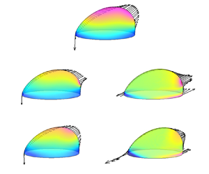
  $Ca=0.35$ at the x–z mid-plane (upper half) and x–y bottom plane (lower half) in the N/N, N/V and V/N systems, where the droplet shapes are represented by the contours ${{\rho }^{N}}=0$.

Figure 3. (a) The steady-state relative wetting area  ${{A}_{r}}$ and relative droplet height ${{h}_{r}}$ and (b) the relative droplet surface area ${{S}_{r}}$ as functions of $Ca$ in three different systems. The inset in (b) shows the steady-state droplet shapes for a representative capillary number of $Ca=0.35$ at the x–z mid-plane (upper half) and x–y bottom plane (lower half) in the N/N, N/V and V/N systems, represented by solid, dashed and dash-dot-dot lines, respectively. The other simulation parameters are $Wi=1.0$, $\beta =0.5$ and $m=1.0$.
With an increase of  $Ca$ in the N/N system, the droplet deforms into a bulge shape in the shear direction (see the inset in figure 3b). The droplet surface area ${{S}_{r}}$ and the wetting area ${{A}_{r}}$ obviously increase, while the droplet height ${{h}_{r}}$ decreases in a small range (figure 3a,b). In the N/V system, ${{S}_{r}}$, ${{A}_{r}}$ and ${{h}_{r}}$ exhibit the same variations in trend with $Ca$ as those in the N/N system. However, the increase in ${{S}_{r}}$ is smaller, ${{A}_{r}}$ spreads more in the $x$ direction and ${{h}_{r}}$ is reduced more rapidly, as compared with the results in the N/N system. In terms of the V/N system, the droplet deforms the least with minimum variations in ${{A}_{r}}$, ${{S}_{r}}$ and ${{h}_{r}}$ among all three systems. In addition, the curvature radius of the contact line appears always larger at the front than at the rear, especially for higher $Ca$ (see the inset in figure 3b) which is consistent with previous findings in a Newtonian system (Ding et al. Reference Ding, Gilani and Spelt2010) and in a surfactant-covered-droplet system (Liu et al. Reference Liu, Zhang, Ba, Wang and Wu2020).
To understand the viscoelastic effect on the steady-state droplet deformation, we compute the traces of the conformation tensor, defined by  $\text {tr}{{\boldsymbol{\mathsf{A}}}}={{A}_{xx}}+{{A}_{yy}}+{{A}_{zz}}$, at $Ca=0.15$ in N/V and V/N systems, and the results are displayed in figure 4. Since $\text {tr}{{\boldsymbol{\mathsf{A}}}}$ is directly proportional to the extension of the polymer molecules (Verhulst et al. Reference Verhulst, Cardinaels, Moldenaers, Renardy and Afkhami2009), one can observe two obvious extension regions, i.e. (I) and (II), in the N/V system (see figure 4a). Region (I) is located near and outside the bulge tip of the droplet, similar to that reported by Verhulst et al. (Reference Verhulst, Cardinaels, Moldenaers, Renardy and Afkhami2009) and Afkhami, Yue & Renardy (Reference Afkhami, Yue and Renardy2009) where the deformation of a Newtonian droplet suspended in viscoelastic matrix subject to simple shear flow was considered. The local extensional flow around the droplet tip leads to severe velocity gradients and increases the stretching of polymer molecules. Region (II) is located around the advancing contact line, where larger velocity gradients are induced by the droplet motion on the stationary bottom wall. In addition, the eigenvector $\boldsymbol {n}_p$ corresponding to the primary eigenvalue of the conformation tensor ${{\boldsymbol{\mathsf{A}}}}$ is often used as an indicator of the orientation of polymer molecules (Yue et al. Reference Yue, Feng, Liu and Shen2005; Aggarwal & Sarkar Reference Aggarwal and Sarkar2007). As an example, figure 4(c) shows the distribution of $\boldsymbol {n}_p$ in the N/V system. It is seen that the polymers around the receding contact line are nearly parallel to the wall, while the polymers around the advancing contact line are distributed on the wall with a large inclination angle to the $x$ direction. Therefore, the polymers near the advancing contact line are easier to be stretched, thus leading to the high values of $\text {tr}{{\boldsymbol{\mathsf{A}}}}$.

Figure 4. Contour plots for  $\text {tr}{{\boldsymbol{\mathsf{A}}}}$ at the x–z mid-plane and the x–y bottom plane in (a) N/V and (b) V/N systems. The dominant polymer orientation $\boldsymbol {n}_p$ presented by line segments with equal length at the x–z mid-plane in (c) N/V and (d) V/N systems. The dashed rectangles with labels (I) or (II) in (a,b) are used to highlight the regions with high $\text {tr}{{\boldsymbol{\mathsf{A}}}}$. The simulation parameters are $Ca= 0.15$, $Wi=1.0$, $\beta =0.5$ and $m=1.0$.
In figure 5, we plot the corresponding distributions of the viscous stress component  ${{( \boldsymbol {n}\boldsymbol {\cdot } {{\boldsymbol {\tau }}_{s}} )}_{x}}$ and the elastic stress component ${{( \boldsymbol {n}\boldsymbol {\cdot } {{\boldsymbol {\tau }}_{p}} )}_{x}}$ on the droplet surface, as well as the vectors of $\boldsymbol {n}\boldsymbol {\cdot } {{\boldsymbol {\tau }}_{s}}$ and $\boldsymbol {n}\boldsymbol {\cdot } {{\boldsymbol {\tau }}_{p}}$ on the droplet interface in the x–z mid-plane, where the results obtained in the N/N system are also displayed for comparison. As a result of the polymer extension, the elastic stress $\boldsymbol {n}\boldsymbol {\cdot } {{\boldsymbol {\tau }}_{p}}$ in the N/V system not only forms a pulling force outside the bulge tip of the droplet, but also expands the bottom wetting area (figure 5b(ii)). In comparison with the N/N system (figure 5a), the viscous stress $\boldsymbol {n}\boldsymbol {\cdot } {{\boldsymbol {\tau }}_{s}}$ in the N/V system is generally smaller, especially in the top region (figure 5b(i)). This is because the Newtonian solvent viscosity of the viscoelastic fluid is only half that of the Newtonian matrix at $\beta =0.5$. Moreover, due to the expansion of the droplet on the wall, the droplet height is reduced, which in turn lowers the viscous stress on the top of the droplet. This can be explained as follows. (1) In Couette flow, the velocity of the ambient fluid increases along the height direction, and the sliding velocity of a droplet is relatively small in the creeping flow condition. Accordingly, when the droplet height gets lower, the velocity difference between the droplet and the ambient fluid at the top surface is smaller, which leads to a lower shear rate and thus a decreased viscous stress. (2) The wall confinement still plays a role in the present problem. For a droplet with lower height, the flow passage that allows the ambient fluid to pass through becomes wider, which decreases the velocity of the ambient fluid near the top of the droplet and also contributes to a decreased viscous stress. On the other hand, even though $\boldsymbol {n}\boldsymbol {\cdot } {{\boldsymbol {\tau }}_{p}}$ contributes to pull the droplet front, it is weak in pushing the droplet rear, leading to a smaller droplet deformation and thus to a lower ${{S}_{r}}$. It is also noticed that the maximum pulling stress $\boldsymbol {n}\boldsymbol {\cdot } {{\boldsymbol {\tau }}_{p}}$ is positioned outside the droplet bulge tip in the N/V system, deviating from the location of the maximum viscous stress $\boldsymbol {n}\boldsymbol {\cdot } {{\boldsymbol {\tau }}_{s}}$ in the N/N system. Such a deviation is attributed to the finite relaxation of the elastic polymer molecules, consistent with previous results obtained from the investigation of a suspended droplet subject to a simple shear flow by Yue et al. (Reference Yue, Feng, Liu and Shen2005), Aggarwal & Sarkar (Reference Aggarwal and Sarkar2008), Verhulst, Moldenaers & Minale (Reference Verhulst, Moldenaers and Minale2007) and Gupta & Sbragaglia (Reference Gupta and Sbragaglia2014).

Figure 5. Contour plots of the normalized  ${{( \boldsymbol {n}\boldsymbol {\cdot } {{\boldsymbol {\tau }}_{s}} )}_{x}}$ on the droplet surface and vector distributions of the normalized $\boldsymbol {n}\boldsymbol {\cdot } {{\boldsymbol {\tau }}_{s}}$ on the interface at the x–z mid-plane for (a) N/N, (b(i)) N/V and (c(i)) V/N. Contour plots of the normalized ${{( \boldsymbol {n}\boldsymbol {\cdot } {{\boldsymbol {\tau }}_{p}} )}_{x}}$ on the droplet surface and vector distributions of the normalized $\boldsymbol {n}\boldsymbol {\cdot } {{\boldsymbol {\tau }}_{p}}$ on the interface at the x–z mid-plane for (b(ii)) N/V and (c(ii)) V/N. The stresses and their $x$ components are all normalized by ${{\mu }_{B}}\dot {\gamma }$. The simulation parameters are $Ca=0.15$, $Wi=1.0$, $\beta =0.5$ and $m=1.0$.
We then analyse the viscoelastic effect in the V/N system. It is seen in figure 4(b) that the polymer extension mainly occurs around the receding contact lines (region (I)) where the polymer molecules exhibit an obvious inclination angle to the bottom wall (figure 4d). A similar strong extension region was numerically obtained in the two-dimensional study of Varagnolo et al. (Reference Varagnolo, Filippi, Mistura, Pierno and Sbragaglia2017). The distributions of  ${{( \boldsymbol {n}\boldsymbol {\cdot } {{\boldsymbol {\tau }}_{s}} )}_{x}}$ in the V/N system (figure 5c(i)) resemble those in the N/N system, but with lower values due to the solvent viscosity difference. Compared with the N/V system, the pulling effect of ${{( \boldsymbol {n}\boldsymbol {\cdot } {{\boldsymbol {\tau }}_{p}} )}_{x}}$ at the droplet front is weaker, and the compressive effect on the droplet rear is almost negligible (figure 5c(ii)). As a consequence, the overall viscous and elastic forces are the lowest and accordingly the droplet deformation is the smallest in the V/N system. With an increase of $Ca$, the droplet deforms more due to an increased stretching effect of $\boldsymbol {n}\boldsymbol {\cdot } {{\boldsymbol {\tau }}_{s}}$ on the droplet tip in all the N/N, N/V and V/N systems. However, the normalized elastic stress is found to vary little with $Ca$ for both N/V and V/N systems. This means that in figure 3, the increase of droplet deformation with $Ca$ in the N/V and V/N systems is mainly attributed to the increased viscous stress.
From the elastic stress vectors at the contact lines, as shown in figure 5(b(ii),c(ii)), it is noticeable that  $\boldsymbol {n}\boldsymbol {\cdot } {{\boldsymbol {\tau }}_{p}}$ in both N/V and V/N systems tends to expand the wetting area. However, compared with the N/N system, an obvious increase in ${{A}_{r}}$ is only observed in the N/V system, and ${{A}_{r}}$ is even lower in the V/N system. What causes a lower ${{A}_{r}}$ in the V/N system? Ramaswamy & Leal (Reference Ramaswamy and Leal1999) pointed out that the viscoelastic effect not only directly acts on the droplet interface through $\boldsymbol {n}\boldsymbol {\cdot } {{\boldsymbol {\tau }}_{p}}$, but also modifies the flow field. Aggarwal & Sarkar (Reference Aggarwal and Sarkar2008) further explained that the flow modification is induced by the viscoelastic stress gradients over the flow domain. To clarify this, we investigate the elastic force $\boldsymbol {\nabla } \boldsymbol {\cdot } {{\boldsymbol {\tau }}_{p}}$ at $Ca= 0.15$ and $Wi=1.0$, and plot the results in figure 6. It is clear that in the N/V system, $\boldsymbol {\nabla } \boldsymbol {\cdot } {{\boldsymbol {\tau }}_{p}}$ at the x–z mid-plane and x–y bottom plane generates outward stretching forces outside the droplet front and in the front and rear contact-line regions, consistent with the effect of $\boldsymbol {n}\boldsymbol {\cdot } {{\boldsymbol {\tau }}_{p}}$ on the droplet deformation. By contrast, in the V/N system, $\boldsymbol {\nabla } \boldsymbol {\cdot } {{\boldsymbol {\tau }}_{p}}$ exhibits severe variation across the rear contact-line region, which is first pointed inward and then outward across the diffuse interface from outside to inside of the droplet. Overall, the inward $\boldsymbol {\nabla } \boldsymbol {\cdot } {{\boldsymbol {\tau }}_{p}}$ in the rear contact-line region is more dominant, thereby inhibiting the spreading of the viscoelastic droplet in the Newtonian matrix.

Figure 6. Vectors of  $\boldsymbol {\nabla } \boldsymbol {\cdot } {{\boldsymbol {\tau }}_{p}}$ at the x–z mid-plane and x–y bottom plane in (a) N/V and (b) V/N systems for $Ca= 0.15$, $Wi=1.0$, $\beta =0.5$ and $m=1.0$. The length of the arrow represents the magnitude of $\boldsymbol {\nabla } \boldsymbol {\cdot } {{\boldsymbol {\tau }}_{p}}$ that is normalized by ${{{\mu }_{B}}\dot {\gamma }}/{R}$. In each panel, the solid contour lines correspond to ${{\rho }^{N}}=0.9$, 0 and $-0.9$, respectively, from inside to outside of the droplet. The vectors at ${{\rho }^{N}}=0$ in the bottom plane are highlighted in red.
In addition to droplet deformation, another meaningful indicator characterizing the droplet behaviour is the sliding velocity of the droplet, which depends on the force balance in the moving direction. Following the arguments by Ding et al. (Reference Ding, Gilani and Spelt2010) and Chen et al. (Reference Chen, Shu, Liu and Zhang2021), the driving force exerted on the droplet interface is balanced by the wall resistance in the  $x$ direction. In the N/V and V/N viscoelastic systems, the driving force is tentatively expressed by the sum of the shear stresses ${{\alpha }_{{{\mu }_{s}}}}{{\mu }_{Bs}}\dot {\gamma }{{R}^{2}}+{{\alpha }_{{{\mu }_{p}}}}{{\mu }_{Bp}}\dot {\gamma }{{R}^{2}}$ and the form drag force ${{\alpha }_{i}}\rho {{R}^{2}}{{( \dot {\gamma }R-{{V}_{cl}} )}^{2}}$, where ${{V}_{cl}}$ is the steady-state sliding velocity of the moving droplet. Assuming that the contact angle hysteresis is neglected, the wall resistance can be written as ${{{\alpha }'}_{{{\mu }_{s}}}}{{\mu }_{Rs}}{{V}_{cl}}R+{{{\alpha }'}_{{{\mu }_{p}}}}{{\mu }_{Rp}}{{V}_{cl}}R$. Thus, the force balance in the $x$ direction is expressed as
 \begin{equation} {{\alpha }_{{{\mu }_{s}}}}{{\mu }_{Bs}}\dot{\gamma }{{R}^{2}}+{{\alpha }_{{{\mu }_{p}}}}{{\mu }_{Bp}} \dot{\gamma }{{R}^{2}}+{{\alpha }_{i}}\rho {{R}^{2}}{{\left( \dot{\gamma }R-{{V}_{cl}} \right)}^{2}}= {{{\alpha }'}_{{{\mu }_{s}}}}{{\mu }_{Rs}}{{V}_{cl}}R+{{{\alpha }'}_{{{\mu }_{p}}}}{{\mu }_{Rp}}{{V}_{cl}}R, \end{equation}
where  ${{{\alpha }'}_{{{\mu }_{s}}}}$, ${{{\alpha }'}_{{{\mu }_{p}}}}$, ${{\alpha }_{{{\mu }_{s}}}}$, ${{\alpha }_{{{\mu }_{p}}}}$ and ${{\alpha }_{i}}$ are the coefficients to be determined, which may be relevant to fluid properties, droplet shape and flow conditions (Chen et al. Reference Chen, Shu, Liu and Zhang2021).
In the N/V system, the parameter  ${{\mu }_{Rp}}$ is zero. Using the definitions of the two-phase fluid viscosity ratio ( $m$) and the solvent viscosity ratio of the matrix fluid ( $\beta$), (4.1) is further derived as
 \begin{equation} \text{N/V:}\quad {{\alpha }_{{{\mu }_{s}}}}\beta {{\mu }_{B}}\dot{\gamma }R+{{\alpha }_{{{\mu }_{p}}}} \left( 1-\beta \right){{\mu }_{B}}\dot{\gamma }R+{{\alpha }_{i}} \rho R{{\left( \dot{\gamma }R-{{V}_{cl}} \right)}^{2}}={{{\alpha }'}_{{{\mu }_{s}}}}m{{\mu }_{B}}{{V}_{cl}}. \end{equation}
By dividing (4.2) by the interfacial tension parameter  $\sigma$, we have
 \begin{equation} \text{N/V:} \quad {{\alpha }_{{{\mu }_{s}}}}\beta Ca+{{\alpha }_{{{\mu }_{p}}}}(1-\beta )Ca+{{\alpha }_{i}} ReCa{{\left( 1-\frac{C{{a}_{cl}}}{Ca} \right)}^{2}}={{{\alpha }'}_{{{\mu }_{s}}}}mC{{a}_{cl}}, \end{equation}
where  $C{{a}_{cl}}$ is the contact-line capillary number defined with ${{V}_{cl}}$ as (Liu et al. Reference Liu, Zhang, Ba, Wang and Wu2020)
 \begin{equation} C{{a}_{cl}}=\frac{{{\mu }_{B}}{{V}_{cl}}}{\sigma }. \end{equation}
The sliding velocity  ${{V}_{cl}}$ is normally much smaller than ${{u}_{w}}$ and the corresponding ${C{{a}_{cl}}}/{Ca}$ is often of $O(10^{-1})$, which means that $({C{{a}_{cl}}}/{Ca})^2$ is a small quantity of $\textit {O}(10^{-2})$ in (4.3). Therefore, the form drag ${{\alpha }_{i}}ReCa{{( 1-{C{{a}_{cl}}}/{Ca} )}^{2}}$ can be simplified as ${{\alpha }_{i}}Ca{( 1-2{C{{a}_{cl}}}/{Ca} )}$ with $Re=1.0$ in the present study. Then, (4.3) for the N/V system is written as
 \begin{equation} \text{N/V:}\quad \frac{C{{a}_{cl}}}{Ca}=\frac{\left( {{\alpha }_{{{\mu }_{s}}}}-{{\alpha }_{{{\mu }_{p}}}}\right) \beta +{{\alpha }_{{{\mu }_{p}}}}+{{\alpha }_{i}}}{{{{{\alpha }'}}_{{{\mu }_{s}}}}m+2{{\alpha }_{i}}}. \end{equation}
Following a similar derivation procedure, the prediction for  ${C{{a}_{cl}}}/{Ca}$ in the V/N system is obtained as
 \begin{equation} \text{V/N:}\quad \frac{C{{a}_{cl}}}{Ca}=\frac{\left( {{{\bar{\alpha }}}_{{{\mu }_{s}}}}- {{{\bar{\alpha }}}_{{{\mu }_{p}}}} \right)\beta +{{{\bar{\alpha }}}_{{{\mu }_{p}}}}+ {{{\bar{\alpha }}}_{i}}}{{{{\bar{{\alpha }}'}}_{{{\mu }_{s}}}}\beta m+{{{\bar{{\alpha }}'}}_{{{\mu }_{p}}}}m \left( 1-\beta \right)+2{{{\bar{\alpha }}}_{i}}}, \end{equation}
where  ${{{\bar {\alpha }}}_{{{\mu }_{s}}}}$, ${{{\bar {\alpha }}}_{{{\mu }_{p}}}}$, ${{{\bar {\alpha }}}_{i}}$, ${{{\bar {{\alpha }}'}}_{{{\mu }_{s}}}}$, ${{{\bar {{\alpha }}'}}_{{{\mu }_{p}}}}$ are the coefficients to be determined for the V/N system. The wall friction in the denominator of (4.6) consists of both viscous and elastic contributions and it is different from that in the N/V system. Under constant $\beta$ and $m$ conditions, $C{{a}_{cl}}$ is expected to vary linearly with $Ca$ for either N/V or V/N system. In particular, the linear relation between $C{{a}_{cl}}$ and $Ca$ has been demonstrated for each two-phase viscosity ratio in the Newtonian system ( $\beta =1.0$) (Ding et al. Reference Ding, Gilani and Spelt2010; Liu et al. Reference Liu, Zhang, Ba, Wang and Wu2020).
To reflect the variation in the sliding velocity, we plot  $Ca_{cl}$ versus $Ca$ for the N/N, N/V and V/V systems in figure 7, where $Wi=1.0$, $\beta =0.5$ and $m=1.0$. As anticipated, the linear relation between $Ca_{cl}$ and $Ca$ is obtained not only in the N/N system, but also in the N/V and V/N systems. By using least-squares linear fitting, the fitted slopes are 0.2236 in the N/N system, 0.2269 in the V/N system and 0.2212 in the N/V system. This means that the droplet is slightly faster in the V/N system but slower in the N/V system when compared with the droplet in the N/N system, which is also reflected in the inset of figure 7. As previously shown in figure 5, the normalized elastic driving force is barely affected by $Ca$, while the viscous driving force in the N/V system is not as strong as that in the V/N system or in the N/N system due to the lower droplet height caused by spreading on the wall. Thus, it leads to a lower slope of $C{{a}_{cl}}$ against $Ca$ in the N/V system. Meanwhile, even though the sum of the driving forces in the V/N system is smaller than that in the N/N system, the corresponding velocity is higher due to lower wall resistance arising from smaller wetting area. With the value of $\beta =0.5$ used in this section, the above analysis indicates that the coefficient $0.5( {{\alpha }_{{{\mu }_{s}}}}+{{\alpha }_{{{\mu }_{p}}}} )$ in the numerator of (4.5) related to driving force is less than ${{\alpha }_{{{\mu }_{s}}}}$ in the N/N system, while the coefficient in the denominator of (4.6) related to wall friction in the V/N system, $0.5( {{{\bar {\alpha }}'}}_{{{\mu }_{s}}}+{{{\bar {\alpha }'}}_{{{\mu }_{p}}}} )$, is smaller than ${{{\bar {\alpha }'}}_{{{\mu }_{s}}}}$ in the N/N system. In Appendix B, we further investigate the variation of $Ca_{cl}$ with $Ca$ in both N/V and V/N systems for varying $Wi$,
$Wi$,  $\beta$ and $m$, and the results are compared with those obtained in the N/N system to show the role of viscoelasticity in the droplet motion.

Figure 7. The contact-line capillary number  $Ca_{cl}$ as a function of the capillary number $Ca$ at $Wi$=1.0, $\beta =0.5$ and $m=1.0$. An inset is included to show a local enlarged view of the $Ca$–
$Ca$– $Ca_{cl}$ plot for $Ca\geq 0.24$. The simulated data are shown by discrete symbols and the fitting lines for the N/N, N/V and V/N systems are represented by solid, dashed and dash-dot-dot lines, respectively.
4.2.2. Effect of  $Wi$
$Wi$

To investigate the effect of viscoelasticity on droplet deformation,  $Wi$ is varied from 0.1, 0.25, 0.5, 1.0, 2.0, 5.0, 8.0 to 10 in the N/V system, and from 0.1, 0.25, 0.5, 1.0, 2.0, 5.0, 10, 20 to 40 in the V/N system. Steady-state droplet deformation with a constant sliding velocity is eventually achieved under various $Wi$ conditions in both N/V and V/N systems. Based on the steady-state results, we plot the contact-line shapes at several representative $Wi$, along with the variations of ${{A}_{r}}$, ${{h}_{r}}$ and ${{S}_{r}}$ with $Wi$ in figure 8.

Figure 8. (a) The steady-state contact-line shapes for  $Wi= 0.1$, 5.0, 10 in the N/V system and for $Wi= 0.1$, 10 in the V/N system. (b) The relative wetting area ${{A}_{r}}$ and relative droplet height ${{h}_{r}}$ and (c) the relative droplet surface area ${{S}_{r}}$ as functions of $Wi$ in the N/V and V/N systems. The other simulation parameters are $Ca=0.15$, $\beta =0.5$ and $m=1.0$.
We first consider the N/V system. As  $Wi$ increases, the wetting area ${{A}_{r}}$ increases and the droplet height ${{h}_{r}}$ decreases monotonically. However, the droplet surface area ${{S}_{r}}$ varies little for $Wi \leq 1.0$, and then obviously increases for $Wi$ above 1.0 (see figure 8b,c). This indicates that the droplet deformation is different from the deformation of a spherical droplet suspended in an Oldroyd-B simple shear flow where the droplet deformation first decreases and then increases with $Wi$ (Yue et al. Reference Yue, Feng, Liu and Shen2005; Aggarwal & Sarkar Reference Aggarwal and Sarkar2008). To understand the cause of the difference, we perform a force analysis at two representative $Wi$ values, i.e. $Wi=0.1$ and 5.0, and the results including the distributions of the normalized viscous stress $\boldsymbol {n}\boldsymbol {\cdot } {{\boldsymbol {\tau }}_{s}}$ and the elastic stress $\boldsymbol {n}\boldsymbol {\cdot } {{\boldsymbol {\tau }}_{p}}$ on the droplet surface, as well as the distributions of the normalized $\boldsymbol {\nabla } \boldsymbol {\cdot } {{\boldsymbol {\tau }}_{p}}$ at the x–z mid-plane and x–y bottom plane, are presented in figure 9.

Figure 9. Vector distributions of  $\boldsymbol {\nabla } \boldsymbol {\cdot } {{\boldsymbol {\tau }}_{p}}$ at the x–z mid-plane and x–y bottom plane for (a) $Wi=0.1$ and(b) $Wi=5.0$; and (c) contour plots of the normalized ${{( \boldsymbol {n}\boldsymbol {\cdot } {{\boldsymbol {\tau }}_{s}} )}_{x}}$ and ${{( \boldsymbol {n}\boldsymbol {\cdot } {{\boldsymbol {\tau }}_{p}} )}_{x}}$ on the droplet surface and vector distributions of the normalized $\boldsymbol {n}\boldsymbol {\cdot } {{\boldsymbol {\tau }}_{s}}$ and $\boldsymbol {n}\boldsymbol {\cdot } {{\boldsymbol {\tau }}_{p}}$ at the x–z mid-plane for $Wi=5.0$ in the N/V system. In (a,b), the solid contour lines correspond to ${{\rho }^{N}}=0.9$, 0 and $-0.9$, respectively, from inside to outside of the droplet. The vectors at ${{\rho }^{N}}=0$ in the bottom plane are highlighted in red. Various stresses or components are normalized by ${{\mu }_{B}}\dot {\gamma }$, while $\boldsymbol {\nabla } \boldsymbol {\cdot } {{\boldsymbol {\tau }}_{p}}$ is normalized by ${{{\mu }_{B}}\dot {\gamma }}/{R}$. The other parameters are chosen as $Ca=0.15$, $\beta =0.5$ and $m=1.0$.
As indicated in Yue et al. (Reference Yue, Feng, Liu and Shen2005) and Aggarwal & Sarkar (Reference Aggarwal and Sarkar2008), the decreased deformation for a suspended droplet at  $Wi \leq 1.0$ in the N/V system is mainly caused by the reduced viscous stretching force due to the decrease in droplet orientation angle caused by elasticity. For the attached droplet in the N/V system with weak elasticity, e.g. $Wi=0.1$, the confinement of the bottom wall resists the droplet rotation. A small difference is observed between the angular position of the maximum ${{( \boldsymbol {n}\boldsymbol {\cdot } {{\boldsymbol {\tau }}_{s}} )}_{x}}$ and that of the maximum ${{( \boldsymbol {n}\boldsymbol {\cdot } {{\boldsymbol {\tau }}_{p}} )}_{x}}$ (similar to figure 5c(i),c(ii) and thus not shown here), which marginally expands the wetting area and lowers the droplet height. Also, the flow modification caused by $\boldsymbol {\nabla } \boldsymbol {\cdot } {{\boldsymbol {\tau }}_{p}}$ is negligible (figure 9a). Both effects lead to a less reduced viscous force $\boldsymbol {n}\boldsymbol {\cdot } {{\boldsymbol {\tau }}_{s}}$, so the droplet deformation quantified by ${{S}_{r}}$ is almost a constant for $Wi \leq 1.0$. After further increasing $Wi$, the increased polymer elasticity in the matrix fluid induces a much stronger stretch locally outside the droplet front (see e.g. $Wi=5.0$ in figure 9c). The locally increased $\boldsymbol {n}\boldsymbol {\cdot } {{\boldsymbol {\tau }}_{p}}$ with $Wi$ was also observed by Aggarwal & Sarkar (Reference Aggarwal and Sarkar2008) for a suspended droplet in simple shear flow. However, it is noted that the maximum $\boldsymbol {n}\boldsymbol {\cdot } {{\boldsymbol {\tau }}_{p}}$ occurs near the droplet tips for a suspended droplet, but around the advancing contact lines for the wall-attached droplet. Such a distribution of $\boldsymbol {n}\boldsymbol {\cdot } {{\boldsymbol {\tau }}_{p}}$ promotes the droplet spreading on the wall, which turns out to exhibit increased ${{A}_{r}}$ and ${{S}_{r}}$ and decreased ${{h}_{r}}$.
On the other hand, the flow modification by  $\boldsymbol {\nabla } \boldsymbol {\cdot } {{\boldsymbol {\tau }}_{p}}$ (figure 9b) acts equally with $\boldsymbol {n}\boldsymbol {\cdot } {{\boldsymbol {\tau }}_{p}}$ in promoting droplet spreading in the N/V system. We also surprisingly find that for $Wi \geq 5.0$ the moving contact line eventually develops into a prolate shape with smaller curvature radius at the front than at the rear (see figures 8a and 9b), which is opposite to the curvature radius distribution of the moving contact line at $Wi =1.0$ (see figure 3b). For high $Wi$, i.e. $Wi \geq 5.0$, the smaller curvature radius at the front is attributed to the fact that $\boldsymbol {\nabla } \boldsymbol {\cdot } {{\boldsymbol {\tau }}_{p}}$ increases rapidly especially near the leading edge of the contact line (see e.g. figure 9b), as opposed to the relatively even distribution of $\boldsymbol {\nabla } \boldsymbol {\cdot } {{\boldsymbol {\tau }}_{p}}$ in the advancing contact line region at $Wi =1.0$ (see e.g. figure 6a).
We then consider the V/N system, and the variations of  ${{A}_{r}}$, ${{h}_{r}}$ and ${{S}_{r}}$ with $Wi$ are given in figure 8. It is clear that increasing $Wi$ slightly decreases the droplet surface area ${{S}_{r}}$ and almost has negligible influence on the wetting area ${{A}_{r}}$ and the droplet height ${{h}_{r}}$. This indicates that the droplet deformation is inhibited to some extent by the droplet viscoelasticity, which is consistent with the trend in the observation obtained for a viscoelastic droplet suspended in a Newtonian shear flow (Aggarwal & Sarkar Reference Aggarwal and Sarkar2007). To elucidate the behaviour of the attached droplet, we plot the distributions of $\boldsymbol {\nabla } \boldsymbol {\cdot } {{\boldsymbol {\tau }}_{p}}$ for $Wi = 0.1$ and 5.0 and $\boldsymbol {n}\boldsymbol {\cdot } {{\boldsymbol {\tau }}_{s}}$, $\boldsymbol {n}\boldsymbol {\cdot } {{\boldsymbol {\tau }}_{p}}$ for $Wi = 5.0$ in figure 10. By comparing these forces, we find that the viscous force $\boldsymbol {n}\boldsymbol {\cdot } {{\boldsymbol {\tau }}_{s}}$ varies little with $Wi$, and the elastic force $\boldsymbol {n}\boldsymbol {\cdot } {{\boldsymbol {\tau }}_{p}}$ mainly acts at the droplet interface near the contact line (see figure 10c). It is also noticed that the increased inward-pointing elastic force $\boldsymbol {\nabla } \boldsymbol {\cdot } {{\boldsymbol {\tau }}_{p}}$ becomes dominant at high $Wi$ (see figure 10b), which overcomes the outward-pointing $\boldsymbol {n}\boldsymbol {\cdot } {{\boldsymbol {\tau }}_{p}}$ and causes the moving contact line to contract in the $x$ direction. As a result, the viscoelastic droplet is squeezed in the $x$ direction but marginally expands in the $y$ direction for high $Wi$, as observed in figure 8(a).

Figure 10. Vector distributions of  $\boldsymbol {\nabla } \boldsymbol {\cdot } {{\boldsymbol {\tau }}_{p}}$ at the x–z mid-plane and x–y bottom plane for (a) $Wi=0.1$ and(b) $Wi=5.0$; and (c) contour plots of the normalized ${{( \boldsymbol {n}\boldsymbol {\cdot } {{\boldsymbol {\tau }}_{s}} )}_{x}}$ and ${{( \boldsymbol {n}\boldsymbol {\cdot } {{\boldsymbol {\tau }}_{p}} )}_{x}}$ on the droplet surface and vector distributions of the normalized $\boldsymbol {n}\boldsymbol {\cdot } {{\boldsymbol {\tau }}_{s}}$ and $\boldsymbol {n}\boldsymbol {\cdot } {{\boldsymbol {\tau }}_{p}}$ at the x–z mid-plane for $Wi=5.0$ in the V/N system. In (a,b), the solid contour lines correspond to ${{\rho }^{N}}=0.9$, 0 and $-0.9$, respectively, from inside to outside of the droplet. The vectors at ${{\rho }^{N}}=0$ in the bottom plane are highlighted in red. Various stresses or components are normalized by ${{\mu }_{B}}\dot {\gamma }$, while $\boldsymbol {\nabla } \boldsymbol {\cdot } {{\boldsymbol {\tau }}_{p}}$ is normalized by ${{{\mu }_{B}}\dot {\gamma }}/{R}$. The other parameters are chosen as $Ca=0.15$, $\beta =0.5$ and $m=1.0$.
To show how  $Wi$ influences the sliding velocity of the droplet in the N/V and V/N systems, we plot the variation of ${C{{a}_{cl}}}/{Ca}$ with $Wi$ in figure 11. It is observed that the variations of ${C{{a}_{cl}}}/{Ca}$ turn out to generally match the variations of ${{A}_{r}}$ displayed in figure 8(b). In both N/V and V/N systems, the wetting area varies little with $Wi$ for $Wi<1.0$, and the sliding velocities are almost a constant. Upon further increasing $Wi$ above unity, ${C{{a}_{cl}}}/{Ca}$ decreases (increases) with an increase (decrease) of ${{A}_{r}}$ in the N/V (V/N) system due to the enhanced (reduced) wall friction.

Figure 11. Plot of  ${C{{a}_{cl}}}/{Ca}$ as a function of $Wi$ in both N/V and V/N systems for $Ca=0.15$, $\beta =0.5$ and $m=1.0$. The simulated results in the N/V and V/N systems are represented by the red triangles and blue circles, respectively. The dashed and dash-dot-dot lines are used to show the variation of ${C{{a}_{cl}}}/{Ca}$ with $Wi$ in the N/V and V/N systems, respectively.
4.2.3. Effect of solvent viscosity ratio $\beta$

In this section, we choose  $Ca=0.15$ and $Wi=1.0$, but decrease $\beta$ from 1.0 to 0.1 at three typical two-phase viscosity ratios, i.e. $m=0.5$, 1.0 and 2.0. Note that for each two-phase viscosity ratio, the elastic effect strengthens with decreasing $\beta$ and vice versa. The droplet deformation is quantified by ${{A}_{r}}$, ${{h}_{r}}$ and ${{S}_{r}}$ in the steady state. The corresponding results in the N/V system are presented in figure 12(a(i),a(ii)). It is seen that a decrease of solvent viscosity ratio $\beta$ leads to an increase in the wetting area ${{A}_{r}}$, but to a decrease in the droplet height ${{h}_{r}}$ and the droplet surface area ${{S}_{r}}$. As anticipated, the elastic force is more pronounced at lower $\beta$, which promotes the droplet spreading on the wall. This will reduce the droplet height, so the droplet is exposed to a weaker shear flow, which reduces the droplet surface area ${{S}_{r}}$. We also notice in figure 12(a(i),a(ii)) that the variations of ${{A}_{r}}$, ${{h}_{r}}$ and ${{S}_{r}}$ with $\beta$ are similar at different values of $m$, while the droplet always deforms the most at $m=2.0$ and the least at $m=0.5$ for each $\beta$. The increased droplet deformation with $m$ was also identified in our previous studies, which considered a clean or surfactant-covered droplet attached on the substrate subject to a Newtonian Couette flow (Liu et al. Reference Liu, Zhang, Ba, Wang and Wu2020). The reason is that a higher droplet viscosity leads to an increased wall friction, which slows down the droplet motion and thus increases the viscous stretching acting on the droplet surface.

Figure 12. Relative wetting area  ${{A}_{r}}$, relative droplet height ${{h}_{r}}$ and relative droplet surface area ${{S}_{r}}$ as functions of decreasing $\beta$ for the two-phase viscosity ratios of $m=0.5$, 1.0 and 2.0 in the (a) N/V and (b) V/N systems. The other parameters are fixed at $Ca=0.15$ and $Wi=1.0$.
We then focus on the V/N system, and investigate the effect of  $\beta$ on ${{A}_{r}}$, ${{h}_{r}}$ and ${{S}_{r}}$ at different values of $m$, which is shown in figure 12(b(i),b(ii)). It is clear in figure 12(b(i)) that ${{A}_{r}}$ and ${{h}_{r}}$ both tend to converge to zero with decreasing $\beta$ for each $m$. The main reason is that the decrease of $\beta$ enhances the droplet elastic effect, which causes the contact line to contract in the $x$ direction (see figure 10b), thus inhibiting the development of wetting area and droplet height. Like in the N/V system, ${{S}_{r}}$ is found to decrease with decreasing $\beta$ as well in the V/N system. However, ${{S}_{r}}$ varies with a steeper slope in the V/N system. The reason is that, on the one hand, $\boldsymbol {n}\boldsymbol {\cdot } {{\boldsymbol {\tau }}_{p}}$ acting as a driving force to promote droplet deformation is smaller and, on the other hand, the inhibiting effect induced by $\boldsymbol {\nabla } \boldsymbol {\cdot } {{\boldsymbol {\tau }}_{p}}$ contributes more at lower $\beta$.
We next investigate how  ${C{{a}_{cl}}}/{Ca}$ is influenced by $\beta$ at three different values of two-phase viscosity ratio in both N/V and V/N systems. The obtained results are shown in figure 13. In the N/V system, it is seen that with a decrease of $\beta$, ${C{{a}_{cl}}}/{Ca}$ monotonically increases for $m=0.5$ and 1.0 but monotonically decreases for $m=2.0$. This means that the presence of viscoelascity in the matrix fluid promotes the droplet motion for $m$ below unity, but inhibits the droplet motion for $m$ above unity. The difference in droplet motion as functions of $\beta$ and $m$ can be explained as follows. As $\beta$ decreases, the elastic viscosity of the matrix fluid increases, which brings two competing effects on the droplet. On the one hand, it promotes the droplet motion through the stretching of the droplet interface. On the other hand, the elastic stretching enlarges the wetting area of the droplet which in turn increases the wall friction. At $m=0.5$ and 1.0 where the wall friction is relatively small due to lower wetting area (see figure 12a(i)) and droplet viscosity, the promoting effect dominates and thus the sliding velocity shows an increasing trend with decreasing $\beta$; whereas at $m=2.0$, the wall friction becomes important so that the sliding velocity decreases with decreasing $\beta$. Unlike that in the N/V system, it is seen in figure 13 that the sliding velocities ( ${C{{a}_{cl}}}/{Ca}$) under three tested $m$ conditions in the V/N system all increase with decreasing $\beta$. As learnt from the droplet deformation trends, it is easier for the droplet to maintain its initial hemispherical shape, droplet height and wetting area at smaller $\beta$. As a result, the droplet would undergo a larger shear force, which promotes the droplet motion and increases the steady-state sliding velocity. In particular, we notice for $\beta <0.4$ that the droplet in the V/N system always slides faster than in the N/V system.

Figure 13. The variation of  ${C{{a}_{cl}}}/{Ca}$ with decreasing $\beta$ for different two-phase viscosity ratios in the N/V and V/N systems. The simulation results are represented by the discrete symbols, i.e. upper-filled symbols for $m=0.5$, open symbols for $m=1.0$ and lower-filled symbols for $m=2.0$, while the predicted curves from (4.5) and (4.6) are represented by dashed, solid and dash-dot-dot lines for $m=0.5$, 1.0 and 2.0, respectively. The other parameters are fixed at $Ca=0.15$ and $Wi=1.0$.
According to (4.5) and (4.6), for each  $m$,
$m$,  ${C{{a}_{cl}}}/{Ca}$ is related to $\beta$ by ${C{{a}_{cl}}}/{Ca}={( \beta +{{a}_{1}} )}/{( {{b}_{1}}m + {{c}_{1}} )}$ in the N/V system and by ${C{{a}_{cl}}}/{Ca}={( \beta +{{a}_{2}} )}/{( {{b}_{2}}m+{{c}_{2}}\beta m +{{d}_{2}})}$ in the V/N system, where ( ${{a}_{1}}$, ${{b}_{1}}$, ${{c}_{1}}$), ( ${{a}_{2}}$, ${{b}_{2}}$, ${{c}_{2}}$, ${{d}_{2}}$) are the fitting parameters related to ( ${{\alpha }_{{{\mu }_{s}}}}$, ${{\alpha }_{{{\mu }_{p}}}}$, ${{\alpha }_{i}}$, ${{{\alpha }'}_{{{\mu }_{s}}}}$, ${{{\alpha }'}_{{{\mu }_{p}}}}$) and ( ${{{\bar {\alpha }}}_{{{\mu }_{s}}}}$, ${{{\bar {\alpha }}}_{{{\mu }_{p}}}}$, ${{{\bar {\alpha }}}_{i}}$, ${{{\bar {{\alpha }}'}}_{{{\mu }_{s}}}}$, ${{{\bar {{\alpha }}'}}_{{{\mu }_{p}}}}$), respectively. By using least-squares fitting on the simulated data in the N/V system, the obtained values of $({{a}_{1}},{{b}_{1}},{{c}_{1}})$ are ( $-$11.34, $-$87.42, $2.98\times 10^{-4}$) for $m=0.5$ (N/V-Case 1), ( $-$27.11, $-$121.18, $-5.06\times 10^{-6}$) for $m=1.0$ (N/V-Case 2) and (24.54, 68.02, $1.79\times 10^{-4}$) for $m=2.0$ (N/V-Case 3). Similarly, the fitting parameters of $({{a}_{2}},{{b}_{2}},{{c}_{2}},{{d}_{2}})$ in the V/N system are (0.14, 0.90, 8.74, 0) for $m=0.5$ (V/N-Case 1), (0.19, 0.73, 4.81, 0) for $m=1.0$ (V/N-Case 2) and (0.37, 0.87, 2.82, 0) for $m=2.0$ (V/N-Case 3). With these fitting parameters, the predicted curves can be obtained, which are plotted in figure 13. Clearly, the simulated results match well with the predicted ones in both N/V and V/N systems, justifying the effectiveness of the derived relationships. Moreover, one easily finds that both ${{c}_{1}}$ and ${{d}_{2}}$ simplified from the coefficients of the form drag term are nearly zero, indicating that the form drag term makes a negligible contribution to the sliding velocity of the droplet under the creeping flow condition for both N/V and V/N systems. Similarly, the form drag term has been commonly neglected in modelling of the droplet motion for the N/N system. For example, Ding & Spelt (Reference Ding and Spelt2008) found that the droplet shape does not have a strong effect on the force balance; Liu et al. (Reference Liu, Zhang, Ba, Wang and Wu2020) established a force balance without considering the form drag term for a system with negligible inertia, and the resulting linear relationship between $Ca_{cl}$ and $Ca$ was numerically verified.
4.3. Breakup of the attached droplet in N/V and V/N systems
It is known in Newtonian systems that an attached droplet could break up into daughter droplets when  $Ca$ is increased above a critical value $Ca_{cr}$, known as the critical capillary number (Ding et al. Reference Ding, Gilani and Spelt2010). In this section, we focus on the variation of $Ca_{cr}$ with $Wi$ in both N/V and V/N systems for $m=1.0$ and $\beta =0.5$. The results are presented in figure 14, where the triangles and circles are used for N/V and V/N systems, respectively, with the open ones representing no-breakup situation and the filled ones representing breakup situation. The critical capillary number $Ca_{cr}$ lies between two nearest filled and open symbols at each $Wi$. The insets show the droplet shapes close to breakup or in steady state for the $Ca$–
$Ca$– $Wi$ conditions enclosed in the corresponding box.

Figure 14. Capillary number at which the droplet obtains a steady shape or undergoes breakup as a function of  $Wi$ for $m=1.0$ and $\beta =0.5$ in the N/V and V/N systems. Each inset shows the droplet shape close to breakup or in the steady state for the cases enclosed in each box. The dashed and dashed-dot-dot lines show the variation of $Ca$ with $Wi$ in the N/V and V/N systems, respectively.
As seen from figure 14,  $Ca_{cr}$ monotonically increases with $Wi$ in the N/V system. The trend is consistent with the droplet deformation results obtained under different values of $Wi$ in § 4.2.2, which can be explained as follows. With an increase of $Wi$, the droplet spreads more on the wall with reduced droplet height, so a larger $Ca_{cr}$ is needed to obtain a driving force sufficient to induce the droplet breakup. To show the influence of $Wi$ on the breakup process, we plot snapshots of droplet breakup in the N/V systems with $Wi=5.0$, $Ca=0.6$ in figure 15(a). By comparing the results with those at lower $Wi$, e.g. $Wi=0.1$ and $Ca=0.435$ in the inset of figure 14, it is seen that the droplet is stretched to be more parallel to the shear flow at higher $Wi$, where the generated daughter droplet is prone to adhering to the wall soon. In addition, we notice an interesting phenomenon at $Wi=10$ in the N/V system, which is shown in the inset of figure 14. The hemispherical droplet eventually develops into a long strip shape at $Ca=0.625$; while at capillary number slightly below $Ca_{cr}$, i.e. $Ca=0.65$, a neck is first formed during the droplet evolution process, and then the embryonic form of the daughter droplet contacts the wall and merges with the main droplet so that no breakup would finally happen.

Figure 15. Snapshots of droplet breakup process for (a)  $Wi=5.0$, $Ca=0.6$ in the N/V system and for(b) $Wi=5.0$, $Ca=0.45$ in the V/N system. The other parameters are fixed at $\beta =0.5$ and $m=1.0$.
In the above discussion, we have shown that the droplet viscoelasticity exhibits an overall inhibiting effect on droplet deformation and the inhibiting effect varies little in the V/N system for  $Wi \geq 10$ (see figure 8). Therefore, one would expect $Ca_{cr}$ to exhibit an increasing trend with $Wi$ before reaching a plateau. However, this expectation only holds for $Wi \leq 2.5$ in the V/N system, which can be seen from the results shown in figure 14. A noticeable difference is that $Ca_{cr}$ undergoes a slight decrease for $Wi$ varying from 2.5 to 5.0. To clarify the cause for the slight decrease of $Ca_{cr}$, we plot the snapshots of droplet breakup for $Wi=5.0$ and $Ca=0.45$ in figure 15(b). It is clear that a larger amount of the droplet is exposed to the shear flow due to smaller wetting area of the droplet at higher $Wi$, which causes the droplet to break up at a lower $Ca_{cr}$.
5. Conclusions
A numerical method is presented to study the deformation and breakup of an attached droplet on a solid wall subject to a three-dimensional Couette flow. Two different systems are considered, namely a N/V system and a V/N system. The numerical method is built upon our recent work (Wang et al. Reference Wang, Wang and Liu2022), which uses the colour-gradient LBM for two-phase hydrodynamics and the advection–diffusion LBM to solve the Oldroyd-B constitutive equation, but additionally introduces the geometrical wetting boundary condition to deal with the fluid–surface interaction. We first focus on low values of capillary number ( $Ca$), and analyse the effects of $Ca$, Weissenberg number $Wi$ and solvent viscosity ratio $\beta$ on the steady-state droplet deformation. In the N/V system, the droplet wetting area increases with an increase of $Ca$ and $Wi$, or with a decrease of $\beta$. In the V/N system, the droplet wetting area decreases with an increase of $Wi$ or a decrease of $\beta$, and the inhibiting effect of the droplet viscoelasticity is strengthened with an increase of $Ca$. The elastic effects are quantified by the elastic stress exerted on the droplet surface, $\boldsymbol {n}\boldsymbol {\cdot } {{\boldsymbol {\tau }}_{p}}$, and the flow modification induced by the elastic force, $\boldsymbol {\nabla } \boldsymbol {\cdot } {{\boldsymbol {\tau }}_{p}}$. It is found that the overall elastic effects of $\boldsymbol {n}\boldsymbol {\cdot } {{\boldsymbol {\tau }}_{p}}$ and $\boldsymbol {\nabla } \boldsymbol {\cdot } {{\boldsymbol {\tau }}_{p}}$ both enhance the droplet spreading in the N/V system. Whereas in the V/N system, the droplet deformation is inhibited by the flow modification $\boldsymbol {\nabla } \boldsymbol {\cdot } {{\boldsymbol {\tau }}_{p}}$, which is dominant over the weak promoting effect of $\boldsymbol {n}\boldsymbol {\cdot } {{\boldsymbol {\tau }}_{p}}$. For the viscoelastic fluid with equal elastic polymer viscosity and Newtonian solvent viscosity, i.e. $\beta =0.5$, the elastic contribution in the V/N system is usually not so strong as the viscous contribution in promoting the interface deformation, so the droplet deformation, quantified by the droplet surface area ${{S}_{r}}$, is smaller than in the Newtonian system. Whereas for the N/V system, ${{S}_{r}}$ varies little for $Wi<1.0$, but obviously increases for higher $Wi$ due the increased elastic driving forces. Decreasing $\beta$ always reduces droplet deformation when either fluid is viscoelastic. A force balance is established for the prediction of the droplet motion (represented by the contact-line capillary number $C{{a}_{cl}}$) in both N/V and V/N systems. Consistent with the theoretical predictions, the numerical simulations not only show that $C{{a}_{cl}}$ linearly increases with $Ca$ in either N/V or V/N system, but also verify the relationship between ${C{{a}_{cl}}}/{Ca}$ and $\beta$ for each two-phase viscosity ratio. In particular, the droplet in the V/N system is found to slide faster than that in the Newtonian system regardless of the two-phase viscosity ratio $m$. Whereas in the N/V system, as compared with the droplet motion in the N/N system, the droplet slides faster for $m<1.0$ but slides more slowly for $m>1.0$. Additionally, the critical capillary number of the droplet breakup, $Ca_{cr}$, is investigated for varying $Wi$ in both N/V and V/N systems. Results reveal that $Ca_{cr}$ evidently increases with $Wi$ in the N/V system, while it first increases and then decreases marginally before reaching a plateau in the V/N system.
Funding
N.W. acknowledges financial support from the National Natural Science Foundation of China (no. 12202344), the Natural Science Basic Research Program of Shaanxi (no. 2022JQ-502) and the Fundamental Research Funds of XJTU (no. xzy012021019). H.L. acknowledges financial support from the National Natural Science Foundation of China (nos. 12072257, 51876170), the National Key Project (no. GJXM92579) and the Major Special Science and Technology Project of the Inner Mongolia Autonomous Region (no. 2020ZD0022).
Declaration of interests
The authors report no conflict of interest.
Appendix A. Effect of wall confinement
To show the effect of wall confinement, a series of simulations are conducted with  $R/H= 0.2$, 0.3, 0.4, 0.5 and 0.625 for $Ca=0.15$, $Wi=1.0$, $\beta =0.5$, $m=1.0$ in the N/N, N/V and V/N systems, and the results are shown in figure 16. It is seen that an increase of wall confinement not only increases the droplet deformation, as quantified by the relative droplet surface area $S_r$, but also enhances the droplet motion (quantified by $Ca_{cl}$) in all three systems. The results also indicate that the effect of the top wall is small enough to be ignored when $R/H \leq 0.3$, consistent with Ding & Spelt (Reference Ding and Spelt2008) where $R/H=0.3$ was used to minimize the role of the top wall and at the same time to keep a relatively low computing cost.

Figure 16. The relative droplet surface area  $S_{r}$ and the contact-line capillary number $Ca_{cl}$ versus the confinement ratio $R/H$ in the N/N, N/V and V/N systems for $Ca=0.15$, $Wi=1.0$, $\beta =0.5$ and $m=1.0$.
Appendix B. Variation of $Ca_{cl}$ with $Ca$ at varying $Wi$, $\beta$ and $m$


In addition to figure 7 ( $Wi=1.0$, $\beta =0.5$, $m=1.0$), more simulations are conduced to show the effect of viscoelasticity on $Ca_{cl}$– $Ca$ curves under different values of $Wi$,
$Wi$,  $\beta$ and $m$ in the N/V and V/N systems. Figure 17 shows the results at $m=1.0$ for two groups of parameters: (i) $\beta =0.1$, $Wi=1.0$ and (ii) $\beta =0.5$, $Wi=5.0$. Note that the groups (i) and (ii) correspond to a lower $\beta$ and to a higher $Wi$, respectively, as compared with the parameters in figure 7. It is found that like in figure 7, the linear relationship between $Ca_{cl}$ and $Ca$ still holds at different $\beta$ and $Wi$ values. However, unlike in figure 7, the slopes are evidently different in the V/N, N/V and N/N systems for either group (i) or group (ii). By keeping $Wi=1.0$, the $Ca_{cl}$– $Ca$ curves are further investigated with $\beta =0.1$ and 0.5 for three typical viscosity ratios, that is, $m=0.25$, 0.5 and 2.0, and the obtained results are displayed in figures 17(b), 17(c) and 17(d), respectively. At each $m$, the corresponding Newtonian results are also plotted for comparison. Clearly, all the $Ca_{cl}$– $Ca$ curves exhibit linear behaviour, and the fitted slopes are listed in table 2. Again, the slopes of the viscoelastic systems are usually different from that of the Newtonian system. In the V/N system, the droplet always slides faster than that in the Newtonian system regardless of the $m$ value. In the N/V system, as compared with the droplet motion in the N/N system, the droplet slides faster for $m<1.0$, but slides more slowly for $m>1.0$. These results suggest that the viscoelasticity generally influences the droplet motion, while the insignificant effect of the viscoelasticity on the droplet motion, as reflected in figure 7, is only a coincidence.

Figure 17. The contact-line capillary number  $Ca_{cl}$ as a function of $Ca$ at (a) $\beta =0.1$, $Wi=1.0$; $\beta =0.5$, $Wi=5.0$ with $m=1.0$, (b) $\beta =0.1$, $Wi=1.0$; $\beta =0.5$, $Wi=1.0$ with $m=0.25$, (c) $\beta =0.1$, $Wi=1.0$; $\beta =0.5$, $Wi=1.0$ with $m=0.5$ and (d) $\beta =0.1$, $Wi=1.0$; $\beta =0.5$, $Wi=1.0$ with $m=2.0$. For the sake of comparison, the corresponding Newtonian results are also plotted in each panel. The simulated data are shown by discrete symbols and the fitted curves for the N/N, N/V and V/N systems are represented by lines of different styles.
Table 2. Fitted slopes of the  $Ca_{cl}$– $Ca$ lines under different parameter conditions.


