2. Dimensional modal and amplitude equations for ring waves

The derivation of the modal and amplitude equations described in this section briefly overviews that given in Khusnutdinova & Zhang (Reference Khusnutdinova and Zhang2016a) but it is developed in dimensional form. Also, we reformulate the boundary conditions assuming that the bottom is at $z = -h$, where h is the undisturbed fluid depth, and the undisturbed surface is at $z=0$, which is customary in oceanographic applications. These modifications aim to make the theory directly applicable in oceanographic contexts.

We consider a ring wave propagating in an inviscid incompressible fluid, described by the full set of Euler equations with the free surface and rigid bottom boundary conditions. Assuming that the waves are long we neglect surface tension. We assume that $u,v,w$ are the velocity components in the $x,y,z$ directions respectively, $p$ is the pressure, $\rho$ is the density of the fluid, $g$ is the acceleration due to gravity, $z=\eta (x,y,t)$ is the height of the free surface (with $z=0$ at the unperturbed surface and $z=-h$ at the flat bottom) and $p_a$ is the atmospheric pressure at the surface. The vertical particle displacement $\zeta$ is used as an additional independent variable, which is defined by the equation

(2.1)\begin{equation} \zeta _t + u\zeta_x +v\zeta_y + w\zeta_z = w ,\end{equation}

and the surface boundary condition

(2.2)\begin{equation} \zeta = \eta \quad \textrm{at}\ z=\eta(x,y,t). \end{equation}

The fluid is in the following basic state:

(2.3a–d)\begin{equation} u_0=u_0(z),\quad v_0=w_0=0,\quad p_{0z}={-} \rho_0 g,\quad \zeta = 0. \end{equation}

Here, $u_0(z)$ is a horizontal shear flow in the $x$-direction and $\rho _0=\rho _0(z)$ is a stable background density stratification.

We introduce the cylindrical coordinate system moving at a constant speed $c$, and use the same notations for the projections of the velocity field on the new coordinate axes

(2.4a–d)$$\begin{gather} x\rightarrow ct+r\cos\theta,\quad y\rightarrow r\sin\theta,\quad z\rightarrow z,\quad t\rightarrow t, \end{gather}$$

(2.5a,b)$$\begin{gather}u\rightarrow u_0(z)+ u\cos\theta -v\sin\theta,\quad v\rightarrow u\sin\theta+v\cos\theta, \end{gather}$$

(2.6a–c)$$\begin{gather}w\rightarrow w,\quad p\rightarrow p,\quad \rho \rightarrow \rho_0+\rho. \end{gather}$$

Then, the equations and boundary conditions take the form

(2.7)\begin{gather} (\rho_0 + \rho) \left [u_t + u u_r + \frac{v}{r} u_{\theta} + w u_z - \frac{v^2}{r} + ((u_0-c) u_r + u_{0z} w) \cos \theta \right. \nonumber\\ \hspace{-9pc}\left . - (u_0-c) (u_{\theta}-v) \frac{\sin \theta}{r}\right ] + p_r = 0, \end{gather}

(2.8)\begin{gather} (\rho_0 + \rho) \left [v_t + u v_r + \frac{v}{r} v_{\theta} + w v_z + \frac{uv}{r} + (u_0-c) v_r \cos \theta \right. \nonumber\\ \hspace{-1pc}\left . - \left ((u_0-c)\left(\frac{v_{\theta}}{r} + \frac{u}{r}\right) + u_{0z} w\right ) \sin \theta \right ] + \frac{p_{\theta}}{r} = 0, \end{gather}

(2.9)$$\begin{gather} (\rho_0 + \rho) \left [ w_t + u w_r + \frac{v}{r} w_{\theta} + w w_z + (u_0-c) \left ( w_r \cos \theta - w_{\theta} \frac{\sin \theta}{r} \right ) \right ]+ p_z + g \rho = 0, \end{gather}$$

(2.10)$$\begin{gather}\rho_t + u \rho_r + \frac{v}{r} \rho_{\theta} + w \rho_z + (u_0-c) \left (\rho_r \cos \theta - \rho_{\theta} \frac{\sin \theta}{r} \right ) + \rho_{0z} w = 0, \end{gather}$$

(2.11)$$\begin{gather}u_r + \frac{u}{r} + \frac{v_{\theta}}{r} + w_z = 0, \end{gather}$$

(2.12)$$\begin{gather}w = \eta_t + u \eta_r + \frac{v}{r} \eta_{\theta} + (u_0-c) \left (\eta_r \cos \theta - \eta_{\theta} \frac{\sin \theta}{r} \right ) \quad \mbox{at}\ z = \eta, \end{gather}$$

(2.13)$$\begin{gather}p = \int_{{-}h}^{\eta} g \rho_0(s)\,\textrm{d} s \quad \mbox{at}\ z = \eta, \end{gather}$$

(2.14)$$\begin{gather}w = 0 \quad \mbox{at}\ z={-}h, \end{gather}$$

with the vertical particle displacement satisfying the following equation and boundary condition:

(2.15)$$\begin{gather} \zeta_t + u \zeta_r + \frac{v}{r} \zeta_{\theta} + w \zeta_z + (u_0-c) \left ( \zeta_r \cos \theta - \zeta_{\theta} \frac{\sin \theta}{r} \right ) = w, \end{gather}$$

(2.16)$$\begin{gather}\zeta = \eta \quad \mbox{at}\ z = \eta. \end{gather}$$

The derivation by Khusnutdinova & Zhang (Reference Khusnutdinova and Zhang2016a) was based on the observation that the linearised equations in the far field ($r\sim {O}(\varepsilon ^{-1})$), where $\varepsilon$ is a small amplitude parameter) admit the modal decomposition (separation of variables) of the form

(2.17)$$\begin{gather} \zeta_1 =A(\xi, R, \theta) \phi(z,\theta), \end{gather}$$

(2.18)$$\begin{gather}u_1 ={-}A\phi u_{0z}\cos\theta - \frac{m \hat F}{m^2+m'^2}A\phi_z, \end{gather}$$

(2.19)$$\begin{gather}v_1 = A\phi u_{0z}\sin\theta - \frac{m' \hat F}{m^2+m'^2}A\phi_z, \end{gather}$$

(2.20)$$\begin{gather}w_1 = A_{\xi} \hat F\phi, \end{gather}$$

(2.21)$$\begin{gather}p_1 =\frac{\rho_0}{m^2+m'^2}A \hat F^2\phi_z, \end{gather}$$

(2.22)$$\begin{gather}\rho_1 ={-}\rho_{0z}A\phi, \end{gather}$$

(2.23)$$\begin{gather}\eta_1 =A\phi \quad \text{at}\ z=0, \end{gather}$$

where $\xi =m(\theta ) r - st$, $R = \varepsilon r m(\theta )$ and $s$ was defined to be the wave speed in the absence of any shear flow (with $m=1$). The function $\phi = \phi (z;\theta )$ is non-dimensional, and it satisfies the following modal equations:

(2.24)$$\begin{gather} \left(\frac{\rho _0 \hat F^2}{m^2 + m'^2} \phi_z \right)_z + \rho_0 N^2 \phi = 0, \end{gather}$$

(2.25)$$\begin{gather}\frac{\hat F^2}{m^2+m'^2}\phi _z - g \phi = 0 \quad\text{at}\ z=0, \end{gather}$$

(2.26)$$\begin{gather}\phi = 0 \quad\text{at}\ z={-}h, \end{gather}$$

where

(2.27a,b)\begin{equation} \hat F = \hat F(z; \theta) ={-}s+(u_0 -c)(m\cos \theta -m'\sin \theta), \quad N^2 ={-} \frac{g \rho_{0z}}{\rho_0}, \end{equation}

with $m=m(\theta )$ and $m'=\textrm {d} m/\textrm {d}\theta$. We fixed the speed of the moving coordinate frame $c$ to be equal to the speed of the shear flow at the bottom of the fluid.

We will refer to the non-dimensional function $m(\theta )$ as the speed modifying function (or simply as the modifying function) for the speed of the ring wave in a particular direction compared with the speed $s$ in the absence of the shear flow, and we shall refer to the corresponding differential equation for this function as the angular adjustment equation (or simply as the angular equation). Indeed, the modified speed of a linear long wave propagating at an angle $\theta$ to the current is ${s}/{m(\theta )}$, and the angular equation can be regarded as the two-dimensional long-wave dispersion relation.

The derivation of the nonlinear amplitude equation was then developed using an asymptotic multiple-scale expansion around this leading-order far-field solution. It was based on the existence of two small parameters; the amplitude parameter $\epsilon =\hat a/h$ and the wavelength parameter $\delta = h/ \lambda$, where $\hat a$ and $\lambda$ are the characteristic amplitude and wavelength. The ‘maximal balance’ condition used to derive the nonlinear amplitude equation is $\delta ^2=\epsilon$. The dimensional form of the equation for the amplitude function $A(\xi , R, \eta )$ is given in Appendix A.

To leading order, the shape of a wavefront in the far field at a distance $r$ from the origin at a fixed moment of time is given by the equation $m(\theta ) r - st = \hbox {const}$, and we require that $m(\theta ) > 0$ considering an outward propagating ring wave. Both $s$ and $m(\theta )$ are to be determined from the solution of the modal equations. The vertical structure of the wave field is also defined by the modal equations. Moreover, the coefficients of the amplitude equation depend on the solution of the modal equations (see Appendix A). Thus, the system of modal equations (2.24)–(2.26) constitutes an important new spectral problem. Solutions for various configurations of the basic stratification and shear flow need to be found in order to make progress in the study of the long three-dimensional ring waves and their generalisations (see § 3). Therefore, our present paper is devoted to the analysis of the modal equations.

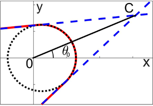
To illustrate, let us first re-consider an example of surface ring waves in a homogeneous fluid with a shear flow (Johnson Reference Johnson1990, Reference Johnson1997) from the viewpoint of the generalised formulation (2.24)–(2.26), and in dimensional form. In particular, let us choose the linear shear flow shown in figure 1. We take the density of the fluid, $\rho _0$, to be a constant, whilst the shear flow is given by $u_0 (z) = \gamma ({(z+h)}/{h})$, where $\gamma$ is a positive constant characterising the surface strength of the current.

Figure 1. Homogeneous fluid with a linear shear current.

We will use this example in order to formulate a rather general sufficient condition ensuring the absence of critical layers, and to introduce quantitative measures for the description of the deformation of the wavefront of a ring wave on a shear current. We will also examine the two-dimensional vertical structure of the ring waves described by the modal functions. This analysis is new since the formalism developed in Johnson (Reference Johnson1990, Reference Johnson1997) was not based on the ideas of modal decomposition.

On solving (2.24) subject to (2.26) we find

(2.28)\begin{equation} \phi = \frac{\varLambda(m^2 + m'^2)}{\rho}\int_{{-}h}^z \frac{1}{\hat F^2} \textrm{d} z = \frac{\varLambda (m^2 + m'^2)(z + h)}{\displaystyle \rho s \left [s - \gamma \frac{z+h}{h} (m\cos\theta - m' \sin\theta)\right ]},\end{equation}

where $\varLambda$ is a parameter which may depend on $\theta$. Then, to satisfy the condition (2.25), we find that the speed modifying function $m$ must satisfy the differential equation

(2.29)\begin{equation} m^2 + m'^2 = \frac{s}{gh} [s - \gamma (m\cos\theta - m' \sin\theta)].\end{equation}

Assuming the absence of a shear flow by setting $\gamma = 0$ and $m = 1$, we have from (2.29) that

(2.30)\begin{equation} s^2 = gh, \end{equation}

thus (2.29) becomes

(2.31)\begin{equation} m^2 + m'^2 = 1 - \frac{\gamma}{s} (m \cos\theta - m' \sin \theta). \end{equation}

This coincides with the generalised Burns condition for this linear shear flow (Johnson Reference Johnson1990, Reference Johnson1997) but is given in dimensional form. It is a nonlinear first-order differential equation which has a general solution of the form

(2.32)\begin{equation} m(\theta) = a \cos \theta + b(a) \sin \theta,\quad \mbox{where}\ b(a) ={\pm} \sqrt{1 - \frac{\gamma}{s} a - a^2}. \end{equation}

It was shown that the solution that describes a ring wave is in fact the envelope of the general solution (so-called singular solution of (2.31)) (Johnson Reference Johnson1990, Reference Johnson1997). This solution is found by requiring that ${\textrm {d} m}/{\textrm {d} a} = 0$, which implies $b'(a) = -({1}/{\tan \theta })$ and allows us to find the singular solution in the form

(2.33)\begin{equation} m(\theta) ={-}\frac{\gamma}{2\sqrt{gh}} \cos\theta \pm \sqrt{1+\frac{\gamma^2}{4gh}}. \end{equation}

The upper sign should be chosen for the outward propagating ring wave, so that $m > 0$ for all values of $\theta$. From this we can recover that, in the absence of a shear flow, with $\gamma = 0\ \textrm {m}\,\textrm {s}^{-1}$, $m(\theta )=1$, a condition that we stated for concentric waves. The general solution (2.32) and its singular solution (2.33) are shown in figure 2(a). The wavefronts for $\gamma = 0\ \textrm {m}\,\textrm {s}^{-1}$, $\gamma = 2\,\textrm {m}\,\textrm {s}^{-1}$ and $\gamma = 5\,\textrm {m}\,\textrm {s}^{-1}$ are shown in figure 2(b). Naturally, for $\gamma = 0\ \textrm {m}\,\textrm {s}^{-1}$, in the absence of a shear flow, the wavefront takes the form of a circle. Increasing the value of $\gamma$ elongates the wavefronts of surface waves in the direction of the current.

Figure 2. (a) The general solution (2.32) for $a =0,\ 0.2,\ 0.4,\ 0.6$ (blue, thin) with its envelope (2.33) (red, thick) for $\gamma = 5\,\textrm {m}\,\textrm {s}^{-1}$. (b) Wavefronts of surface ring waves. The black (solid) curve is for $\gamma = 0\,\textrm {m}\,\textrm {s}^{-1}$, the red (dash) curve for $\gamma = 2\,\textrm {m}\,\textrm {s}^{-1}$ and the blue (dot) curve for $\gamma = 5\,\textrm {m}\,\textrm {s}^{-1}$. Here, $g = 9.8\,\textrm {m}\,\textrm {s}^{-2}$, $h = 10$ m and $r m(\theta ) = 5000$ m.

A critical layer occurs when $\hat F(z, \theta ) = 0$. Consider $\hat F_{\theta } = - (u_0 - c) (m + m'') \sin \theta$. Let us assume that $u_0 - c > 0$, i.e. there are no current reversals, which is the case in the example above and in all subsequent examples. We shall consider a singular solution satisfying $m + m'' > 0$, i.e. an outward propagating wave. Indeed, such a wave in the absence of any current is described by $m = 1$, therefore $m+m'' > 0$ for a sufficiently weak current, by continuity. Then, $\hat F_\theta < 0$ if $\theta \in (0, {\rm \pi})$ and $\hat F_\theta > 0$ if $\theta \in ({\rm \pi} , 2 {\rm \pi})$. Therefore, $\hat F$ will reach a maximum at $\theta = 0$. Thus, to avoid critical layers we require

(2.34)\begin{equation} \hat F \le \hat F|_{\theta = 0} ={-} s + (u_0 - c) m(0) < 0, \end{equation}

implying $(u_0-c) m(0) < s$. Here, ${s}/{m(0)} \ge s$ is the downstream wave speed, implying

(2.35)\begin{equation} u_0 - c < s \le \frac{s}{m(0)}. \end{equation}

Thus, the inequality $u_0 - c < s$ is a simple, and rather general, sufficient condition for the absence of critical layers, generalising the condition formulated by Khusnutdinova & Zhang (Reference Khusnutdinova and Zhang2016a) for a piecewise-constant current. The inequality $u_0 - c < {s}/{m(0)}$ is less restrictive, and this is the necessary and sufficient condition. It requires the knowledge of $m(0)$. Both conditions are applicable to all examples in this paper, and there are no critical levels. In particular, for the present example, $u_0 = \gamma ({(z+h)}/{h})$, and we obtain the sufficient condition

(2.36)\begin{equation} \gamma < \sqrt{gh}. \end{equation}

The necessary and sufficient condition reads

(2.37)\begin{equation} \gamma < \frac{\sqrt{gh}}{\displaystyle - \frac{\gamma}{2 \sqrt{gh}} + \sqrt{1+ \frac{\gamma^2}{4 gh}}}. \end{equation}

Next, we shall introduce a measure of the deformation of the wavefront. This can be done globally, for the whole ring wave, considering the distance between the points on the wavefront in the downstream and upstream directions, i.e.

(2.38)\begin{equation} D_{\gamma} = \frac{st}{m(0)} + \frac{st}{m({\rm \pi})}, \end{equation}

and comparing this distance to a similar distance in the absence of the shear flow, $D_0 = 2st$. It is natural to consider the ratio

(2.39)\begin{equation} \frac{D_{\gamma}}{D_0} = \frac 12 \left (\frac{1}{m(0)} + \frac{1}{m({\rm \pi})} \right ). \end{equation}

Here, $m(\theta )$ is given by (2.33). The plot of this global measure as a function of the strength of the current is shown in figure 3(a). It might be also helpful to show the plots of the ratios of the speeds of the wavefront at $\theta = 0$ and $\theta = {\rm \pi}$ (downstream and upstream directions) to the speed $s$ in the absence of any current. This can be seen in figure 3(b), where the upstream speed has been shifted upwards by 2 units, for a better comparison with the downstream speed. Both plots give a clear indication of a significant elongation of the wavefront in the direction of the current.

Figure 3. (a) Relative distance between the points on the wavefronts of surface ring waves in downstream and upstream directions as a function of $\gamma$. (b) Relative speed of the wavefronts of surface ring waves in downstream and upstream directions as a function of $\gamma$. The blue (solid) curve is for $\theta = 0$ (downstream) and the red (dash) curve for $\theta = {\rm \pi}$ (upstream). Here, $g = 9.8\,\textrm {m}\,\textrm {s}^{-2}$ and $h = 10$ m. (The upstream speed has been shifted upwards by 2 units.).

However, in many satellite images the oceanic internal waves propagate as a part of a ring and not the whole ring (see, for example, figure 1 in Khusnutdinova & Zhang (Reference Khusnutdinova and Zhang2016a) or figure 13 in Apel Reference Apel2003). Therefore, it is desirable to introduce a local measure of the deformation of the wavefront. This can be done by introducing the geometric curvature of the wavefront, which in polar coordinates is given by (e.g. Da Cormo Reference Da Cormo2017)

(2.40)\begin{equation} k_{ \gamma} = \frac{|r^2 + 2 r'^2 - r r''|}{(r^2 + r'^2)^{3/2}}, \quad \mbox{where}\ r = r(\theta). \end{equation}

Applying this formula to $r(\theta ) = {st}/{m(\theta )}$ we obtain

(2.41)\begin{equation} k_{\gamma} = \frac{|m + m''|}{st \left [1 + \left ({\displaystyle \frac{m'}{m}} \right )^2 \right ]^{3/2}}. \end{equation}

In the absence of any current, $m(\theta )= 1$ and $k_0 (\theta ) = (st)^{-1}$. Taking the ratio,

(2.42)\begin{equation} \frac{k_{\gamma}}{k_0} = \frac{|m + m''|}{\left [1 + \left ({\displaystyle \frac{m'}{m}} \right )^2 \right ]^{3/2}}, \end{equation}

which in the present example gives

(2.43)\begin{equation} \frac{k_{\gamma} (\theta)}{k_0 (\theta)} = \frac{\sqrt{\displaystyle 1 + \frac{\gamma^2}{4 s^2}}}{ G^{3/2}}, \quad \mbox{where}\ G = 1 + \frac{\gamma^2}{4 s^2} \frac{\sin^2 \theta}{\displaystyle \left ( \sqrt{1 + \frac{\gamma^2}{4 s^2}} - \frac{\gamma \cos \theta}{2 s} \right )^2 }. \end{equation}

The plot of this local measure as a function of the strength of the current is shown for $\theta = 0, {{\rm \pi} }/{2}$ and ${\rm \pi}$ in figure 4. We can see that the curvature is growing in the upstream and downstream directions, while it is decreasing in a transverse direction, giving a clear indication (and quantitative measure) of the elongation of the wavefront compared with the concentric wavefront in the absence of the current.

Figure 4. Relative curvature of the wavefronts of surface ring waves in different directions as a function $\gamma$. The blue (solid) curve is for $\theta = 0$, the black (dash-dot) curve for $\theta = {{\rm \pi} }/{2}$ and the red (dash) curve for $\theta = {\rm \pi}$. Here, $g = 9.8\,\textrm {m}\,\textrm {s}^{-2}$ and $h = 10$ m.

Note that, in accordance with the Gauss–Bonnet theorem for closed convex curves (e.g. Da Cormo Reference Da Cormo2017), the curvature (a time-dependent function) satisfies the relation

(2.44)\begin{equation} \oint k_{\gamma}\,\textrm{d} s = 2{\rm \pi},\end{equation}

which yields the total curvature conservation law in the following general form:

(2.45)\begin{equation} \oint k_{\gamma} \,\textrm{d} s = \int_0^{2 {\rm \pi}} k_{\gamma} (\theta) \sqrt{r^2 + r'^2} \,\textrm{d}\theta = \int_0^{2 {\rm \pi}} \frac{m\ |m + m''|}{m^2 + m'^2} \textrm{d}\theta = 2{\rm \pi}. \end{equation}

This conservation law can be used, for example, to control the accuracy of computer assisted plots of the wavefronts of ring waves, which becomes essential in some complicated cases (in particular, we used it for the flows considered in § 5, having fixed an error in Khusnutdinova Reference Khusnutdinova2020).

It is also instructive to examine the two-dimensional structure of the modal function (2.28). Before we can do this, the parameter $\varLambda$ must be determined. We normalise $\phi$ by setting $\phi = 1$ at $z = 0$. This gives

(2.46)\begin{equation} \varLambda = \rho g, \end{equation}

which is independent of $\theta$. Thus,

(2.47)\begin{equation} \phi = \frac{g (m^2+m'^2) (z+h)}{\displaystyle s \left [\displaystyle s - \gamma \frac{z+h}{h} (m \cos \theta - m' \sin \theta)\right ] }, \end{equation}

and the modal function is shown in figure 5 for $\theta = 0, {\rm \pi}, {\rm \pi}/{2}$, i.e. in the downstream, upstream and orthogonal directions, respectively. The current has the effect of a similar magnitude in the downstream and upstream directions, while the effect in the orthogonal direction to the current is expectedly weak. We conclude that the vertical structure of the wave field is shifted towards the surface in the downstream direction, and towards the ocean bottom in the upstream direction.

Figure 5. Plots of the modal function (2.28) for $\gamma = 0\,\textrm {m}\,\textrm {s}^{-1}$ (black, solid), $\gamma = 2\,\textrm {m}\,\textrm {s}^{-1}$ (red, dash) and $\gamma = 5\,\textrm {m}\,\textrm {s}^{-1}$ (blue, dot). Here, $g = 9.8\,\textrm {m}\,\textrm {s}^{-2}$ and $h = 10$ m. (a) $\theta = 0$ (downstream); (b) $\theta = {\rm \pi}$ (upstream) and (c) $\theta = {\rm \pi}/2$ (orthogonal).

3. Derivation of modal equations from the formulation for plane waves

The aim of this section is to arrive at the modal equations (2.24)–(2.26) starting from the equations for the plane waves. This allows us to clarify the roles of the general solution of the angular adjustment equation and its envelope, provides a natural way of describing important properties of the ring waves (e.g. their group speed) and allows us to outline an analytical approach to constructing more general hybrid wavefronts consisting of an arc of a ring wave and two tangent plane waves.

Since the terms of interest are linear and in the long-wave regime, it is sufficient to consider only the linear long-wave equations. Relative to a background shear flow $u_{0}(z)$ and a background density field $\rho _{0}(z)$, the equations are in the same domain $-h < z < 0$, and in standard notation,

(3.1)$$\begin{gather} \rho_0 (u_t + u_0 u_x + u_{0z}w ) + p_x = 0, \end{gather}$$

(3.2)$$\begin{gather}\rho_0 (v_t + u_0 v_x ) + p_y = 0, \end{gather}$$

(3.3)$$\begin{gather}p_{z}+g\rho = 0 , \end{gather}$$

(3.4)$$\begin{gather}\rho_t + u_0 \rho_{x } + w\rho_{0z} = 0, \end{gather}$$

(3.5)$$\begin{gather}u_{x} + v_{y} + w_{z} = 0 , \end{gather}$$

(3.6)$$\begin{gather}\zeta_t + u_{0} \zeta_x - w =0 . \end{gather}$$

The boundary conditions are

(3.7)$$\begin{gather} p -g\rho_{0} \zeta = 0 \quad \hbox{at}\ z = 0, \end{gather}$$

(3.8)$$\begin{gather}w =0 \quad \hbox{at}\ z={-}h. \end{gather}$$

Since the only inhomogeneity is the $z$-dependence in $u_{0}, \rho _{0}$, it is convenient to look at the linear long-wave theory in Fourier space, for a disturbance proportional to $\exp {(\textrm {i}kx +\textrm {i}ly - \textrm {i}k\tilde ct)}$, i.e.

(3.9)\begin{equation} (u,v,w,p,\rho, \zeta) = (\tilde u, \tilde v, \tilde w, \tilde p,\tilde \rho, \tilde \zeta) \exp({\textrm{i} (k x + l y - k \tilde c t)}) + c.c. \end{equation}

Then (3.1)–(3.6) become, after eliminating $\tilde w, \tilde \rho$,

(3.10)$$\begin{gather} \rho_0 [-\textrm{i}k(\tilde c-u_0)(\tilde u + u_{0z }\tilde \zeta)] + \textrm{i}k\tilde p =0, \end{gather}$$

(3.11)$$\begin{gather}\rho_0 [-\textrm{i}k(\tilde c-u_0)\tilde v] + \textrm{i}l \tilde p =0, \end{gather}$$

(3.12)$$\begin{gather}\textrm{i}k\tilde u + \textrm{i}l\tilde v - \textrm{i}k[(\tilde c-u_0) \tilde \zeta]_z =0, \end{gather}$$

(3.13)$$\begin{gather}\rho_0 N^2 \tilde \zeta + \tilde p_z = 0. \end{gather}$$

Next, we use (3.11), (3.12) to eliminate $\tilde u, \tilde v$ and so obtain in place of (3.10), (3.11),

(3.14)\begin{equation} \rho_{0}[-\textrm{i}k(\tilde c-u_0)^2 \tilde \zeta_z] + \textrm{i}k \left (1 + \frac{l^2}{k^2 }\right ) \tilde p=0. \end{equation}

Together with (3.13) these equations form two equations for $\tilde \zeta , \tilde p$. The final step is to eliminate $\tilde p$ between (3.13) and (3.14) to obtain

(3.15)\begin{equation} [\rho_{0}(\tilde c-u_0)^2 \tilde \zeta_z ]_z + \rho_{0}N^2 \left (1 + \frac{l^2}{k^2} \right )\tilde \zeta = 0. \end{equation}

The boundary conditions (3.7), (3.8) are similarly reduced to

(3.16)$$\begin{gather} (\tilde c-u_0)^2 \tilde \zeta_z = \left (1+ \frac{l^2}{k^2} \right ) g \tilde \zeta \quad \hbox{at}\ z = 0, \end{gather}$$

(3.17)$$\begin{gather}\tilde \zeta =0 \quad \hbox{at}\ z={-}h. \end{gather}$$

Next, we can write $\tilde \zeta = A(k, l)\phi (z)$ and so

(3.18)\begin{equation} [\rho_0 (\tilde c-u_0)^2 \phi_z]_z + \rho_0 N^2 \left (1 + \frac{l^2}{k^2}\right )\phi = 0, \end{equation}

subject to the boundary conditions

(3.19)\begin{equation} (\tilde c-u_0)^2 \phi_z = g \left (1 + \frac{l^2 }{k^2 } \right )\phi \quad \hbox{at}\ z =0,\quad \hbox{and}\quad \phi = 0 \quad \hbox{at}\ z ={-}h. \end{equation}

The speed $\tilde c$ and the modal function now retain a dependence on $k, l$, which is removed in the one-dimensional case when $l =0$. The KP equation follows when $l^2 \ll k^2$ and again this reduces to the usual modal equation where, at leading order, $\tilde c$ is a constant. In the general case when there is a shear flow $u_{0}(z) \ne \hbox {const}$, the dispersion relation is not isotropic.

It is useful to note that the integral identity readily obtained from the modal equation in the case of continuous stratification,

(3.20) \begin{align} \mathcal{D} (\omega, \boldsymbol{k}) = \int_{{-}h}^{0}\rho_{0} \left [k^2 (\tilde c-u_0)^2 \phi_{z}^2 - N^{2}(k^2 + l^2)\phi^2\right]\textrm{d} z - [\rho_0 g (k^2 + l^2)\phi^2 ]_{z=0} = 0, \end{align}

can be regarded as the dispersion relation, recalling that $\omega =k \tilde c$ and $k (\tilde c - u_0) = \omega - ku_{0}$.

More generally, $k, l$ may be defined as local wavenumbers depending on $x, y$, in the spirit of Whitham (Reference Whitham1999), and then the wavefronts become the curves

(3.21)\begin{equation} S (x, y, t) = \hbox{const},\quad \mbox{where}\ k=S_x,\quad l = S_y,\enspace \omega ={-} S_t. \end{equation}

They can be determined by solving the equations

(3.22a–c)\begin{equation} k_t + \omega_x = 0,\quad l_t + \omega_y = 0,\quad k_y = l_x,\quad \hbox{where}\ \omega = \omega (k, l). \end{equation}

Here, the third equation is only required at $t=0$ since the first two equations imply that $(k_y - l_x)_t = 0$. Next, in order to change to a reference frame moving with a known speed $c$, we need to use a Galilean transformation which in effect replaces $u_{0}$ with $u_{0} - c$.

Let us now use the above to recover the modal equations for the ring waves described in the previous section. In polar coordinates, the wavefronts are described by

(3.23)\begin{equation} S=S(r, \theta, t) = \hbox{const}, \end{equation}

where $x = r\cos {\theta },\ y= r\sin {\theta }$. Then, we define

(3.24a,b)\begin{equation} \hat \gamma = S_r,\quad \hat \sigma = \frac{S_{\theta}}{r}, \end{equation}

where

(3.25a–c)\begin{equation} \hat \gamma_t + \omega_r = 0,\quad r \hat \sigma_t + \omega_{\theta} = 0,\quad \hat \gamma_{\theta}= (r \hat \sigma )_r. \end{equation}

The local wave vector $\boldsymbol {k} = (k, l)$ in Cartesian coordinates becomes the local wave vector in polar coordinates, $\boldsymbol {k} = \hat \gamma \hat {r} + \hat \sigma \hat {\theta }$ where $\hat {r} = (\cos {\theta }, \sin {\theta })$ and $\hat {\theta } = (-\sin {\theta }, \cos {\theta })$ are unit vectors in the radial and polar angle directions, respectively. Hence

(3.26a,b)\begin{equation} k = \hat \gamma \cos{\theta} - \hat \sigma \sin{\theta},\quad l = \hat \gamma \sin{\theta} + \hat \sigma \cos{\theta}.\end{equation}

We can define $\hat \gamma = \kappa \cos {\beta },\ \hat \sigma = \kappa \sin {\beta }$ so that $k= \kappa \cos {\alpha },\ l = \kappa \sin {\alpha }$, and $\kappa = |\boldsymbol {k}| = (\hat \gamma ^2 + \hat \sigma ^2 )^{1/2}$ is the wave vector magnitude. Here, $\alpha = \theta + \beta$, where $\beta$ is the angle between the vectors $\boldsymbol {k}$ and $\hat {r}$. Then, the modal equations (3.18), (3.19) become

(3.27)$$\begin{gather} [\rho_0 k^2 (\tilde c - u_0)^2 \phi_z ]_z + \rho_0 N^2 \kappa^2 \phi = 0, \end{gather}$$

(3.28)$$\begin{gather}k^2 (\tilde c - u_0)^2 \phi_z = g\kappa^2 \phi \quad \hbox{at}\ z =0,\quad \hbox{and}\quad \phi = 0 \quad \hbox{at}\ z ={-}h. \end{gather}$$

Here, $\kappa , k$ can be expressed in terms of $\hat \gamma , \hat \sigma ; \theta$, and the dispersion relation generally, for a piecewise-continuous stratification, can be expressed in the form

(3.29)\begin{equation} \omega (\hat \gamma, \hat \sigma; \theta) = k \tilde c(k, \kappa^2). \end{equation}

In the case of continuous stratification, the dispersion relation can be expressed in the form,

(3.30a,b)\begin{equation} \omega (\hat \gamma, \hat \sigma; \theta) = k \tilde c(\sec^2{\alpha}),\quad \sec{\alpha} = \frac{\kappa}{k}, \end{equation}

or in the integral form

(3.31)\begin{equation} \left.\begin{gathered} \mathcal{D} (\omega, \hat \gamma, \hat \sigma; \theta) = \int_{{-}h}^{0}\rho_{0}[k^2 (\tilde c - u_0)^2 \phi_{z}^2 - N^{2} \kappa^2 \phi^2]\textrm{d} z - [\rho_0 g \kappa^2 \phi^2 ]_{z=0} = 0, \\ k (\tilde c - u_0) = \omega - ku_{0} = \omega - (\hat \gamma \cos{\theta} - \hat \sigma \sin{\theta})u_{0},\quad \kappa^2 = \hat \gamma^2 + \hat \sigma^2. \end{gathered}\right\} \end{equation}

For instance, if we choose to write, as in the previous section,

(3.32)\begin{equation} S = m r - s t, \end{equation}

where $m = m(\theta )$ and $s$ is a constant speed in the absence of the shear flow, then

(3.33a–c)\begin{equation} \hat \gamma= m,\quad \hat \sigma = m' \quad \mbox{and} \quad \omega = s. \end{equation}

The wavefronts of the ring waves are given by $m r - s t = const$ , with

(3.34a–c)\begin{equation} \kappa^2 = m^2 + m'^2,\quad k = m \cos{\theta } - m' \sin{\theta },\quad l = m \sin \theta + m' \cos \theta. \end{equation}

The modal equations (3.27), (3.28) take the form

(3.35)$$\begin{gather} (\rho_0 \hat F^2 \phi_z )_z + \rho_0 N^2 (m^2 + m'^2)\phi = 0, \end{gather}$$

(3.36)$$\begin{gather}\hat F^2 \phi_z = g(m^2 + m'^2)\phi \quad \hbox{at}\ z =0,\quad \hbox{and}\quad \phi = 0 \quad \hbox{at}\ z ={-}h, \end{gather}$$

where

(3.37)\begin{equation} \hat F ={-} k (\tilde c - u_0) ={-}s + u_{0}(m \cos{\theta } - m' \sin{\theta }), \end{equation}

which in the reference frame moving with the speed $c$ becomes

(3.38)\begin{equation} \hat F ={-} k (\tilde c - u_0) ={-}s + (u_{0} - c) (m \cos{\theta } - m' \sin{\theta }). \end{equation}

These equations are equivalent to the modal equations (2.24)–(2.26) from the previous section. It is important to note that here the modal equations are defined locally, and the relevant solutions of the corresponding angular equation associated with the modal equations are members of the general solution, which clarifies their role as solutions describing the plane waves tangent to the ring wave. The existence of the far-field modal decomposition for the ring waves is a global result. The relevant solution is the singular solution of the same angular equation.

In the case of continuous stratification, the dispersion relation (3.29) with $\kappa , k$ given by (3.34a–c) takes the form

(3.39) \begin{equation} s = (m \cos{\theta } - m' \sin{\theta })\tilde c[(m^2 + m'^2)/ (m \cos{\theta } - m' \sin{\theta })^2], \end{equation}

and may be written in the integral form (3.31) as

(3.40) \begin{align} \mathcal{D} (s, m, m'; \theta )= \int_{{-}h}^{0}\rho_{0} [\hat F^2 \phi_{z}^2 - N^{2}(m^2 + m'^2)\phi^2]\,\textrm{d} z - [\rho_0 g (m^2 + m'^2)\phi^2 ]_{z=0} = 0. \end{align}

In general, the angular equation (3.39) forms a rather complicated ordinary differential equation for $m (\theta )$ since $\hat F = \hat F(z; \theta )$. We will analyse its solutions for the cases of a two-layered fluid with the linear current and a power-law upper-layer current in the next sections.

Here, we consider another simple example. Suppose that $N = \hbox {const}$. Then, for ${u_{0} (z) = 0}$, and in the Boussinesq and rigid-lid approximations, the solution of the modal equations is given by

(3.41)\begin{equation} \phi = \varLambda \sin \frac{n {\rm \pi}z}{h}, \quad \mbox{where}\ n = 1,2,3, \ldots, \end{equation}

where

(3.42)\begin{equation} m^2 + m'^2 = \left ( \frac{n {\rm \pi}s}{Nh} \right )^2. \end{equation}

The parameter $\varLambda$ can be used to normalise the modal function to be equal to one at some level of interest. Here, since there is no shear flow, $m=1$, and then (3.42) implies that

(3.43)\begin{equation} s = \frac{Nh}{{\rm \pi} n}, \quad \mbox{where}\ n = 1,2,3, \ldots, \end{equation}

describing the speeds of the concentric ring waves. It is instructive also to consider the general solution of (3.42), which is given by

(3.44)\begin{equation} m = a \cos \theta + b(a) \sin \theta, \quad \mbox{where}\ a^2 + b^2 = \left ( \frac{n {\rm \pi}s}{Nh} \right )^2, \end{equation}

as these solutions describe plane waves propagating at an arbitrary angle

(3.45)\begin{equation} S = m r - s t = [a \cos \theta + b(a) \sin \theta] r - s t = ax + b y - st, \end{equation}

where

(3.46)\begin{equation} s^2 = \frac{Nh}{{\rm \pi} n} \sqrt{a^2 + b^2},\quad a = k,\ b = l,\quad \mbox{and}\quad \boldsymbol{k} = (k, l). \end{equation}

Looking for a singular solution, we re-parametrise the general solution as

(3.47a,b)\begin{equation} m = \frac{n {\rm \pi}s}{Nh} \cos (\varTheta - \theta),\quad \left(a = \frac{n {\rm \pi}s}{Nh} \cos \varTheta,\ b = \frac{n {\rm \pi}s}{Nh} \sin \varTheta\right), \end{equation}

and then find the envelope of this general solution, by requiring that ${\textrm {d} m}/{\textrm {d} \varTheta } = 0,$ which immediately yields $m = 1$. The case when $u_0(z) = U_0 = \hbox {const}$ can be reduced to the previous case by a Galilean transformation, and therefore again describes concentric ring waves in a reference frame moving with the speed $c=U_0$.

Next, it is useful to obtain the group velocity and the wave action conservation law related to the ring waves. This can be done working with the local wave numbers given by the formulae (3.34a–c). The wave action conservation law is expressed by

(3.48)\begin{equation} \mathcal{A}_t + \boldsymbol{\nabla}\boldsymbol{\cdot} (\tilde{\boldsymbol{c}}_g \mathcal{A} ) = 0, \end{equation}

where the group velocity $\tilde {\boldsymbol {c}}_g = (\omega _k , \omega _l )$ and $\mathcal {A}$ is the wave action density (e.g. Whitham Reference Whitham1999), given in the long-wave limit by

(3.49)\begin{equation} \mathcal{A} = \int_{{-}h}^{0} \rho_{0} (\tilde c - u_0) |A|^2 \phi_{z}^2 \,\textrm{d} z. \end{equation}

In the case of continuous stratification, since $\omega =\omega (k,l)= k\tilde c = k\tilde c [(k^2 + l^2)/k^2]$, we have

(3.50)\begin{equation} \tilde{\boldsymbol{c}}_g = \left(\tilde c - \tilde c_{\hat \xi} \frac{2l^2}{k^2}, \tilde c_{\hat \xi}\frac{2l}{k}\right),\quad \hat \xi = 1 + \frac{l^2}{k^2 }. \end{equation}

The integral form (3.20) can be used to obtain

(3.51)\begin{equation} \mathcal{D}_{\omega} \tilde{\boldsymbol{c}}_g + \boldsymbol{\nabla}_{\boldsymbol{k}} \boldsymbol{\cdot} \mathcal{D} = 0. \end{equation}

As an example, we shall consider the outward propagating surface ring waves over a linear current shown in figure 1. The angular adjustment equation is given by (2.29) and can be rewritten in the form

(3.52)\begin{equation} \kappa^2 = \frac{s^2}{gh} - \frac{\gamma s}{gh} k, \end{equation}

leading, on choosing a positive root of the quadratic equation for $s$, to the formula

(3.53)\begin{equation} \omega = k \tilde c = s = \sqrt{gh \left ( \sigma^2 k^2 + l^2 \right )} + \frac{\gamma k}{2},\quad \sigma^2 = 1 + \frac{\gamma^2}{4gh}. \end{equation}

Then, we can define the phase velocity of the plane waves tangent to the ring waves as

(3.54)\begin{equation} \tilde{\boldsymbol{c}}_{\boldsymbol{p}} = \frac{\omega}{\kappa^2} \boldsymbol{k}, \end{equation}

where the local wave vector is given in Cartesian coordinates by

(3.55)\begin{align} \boldsymbol{k} &= (k, l) = (m \cos \theta - m' \sin \theta, m \sin \theta + m' \cos \theta) \nonumber\\ &= \left (- \frac{\gamma}{2 \sqrt{gh}} + \sigma \cos \theta, \sigma \sin \theta \right ), \end{align}

and in polar coordinates by

(3.56)\begin{equation} \boldsymbol{k} = (\hat \gamma, \hat \sigma) = (m, m') = \left ( \sigma -\frac{\gamma}{2\sqrt{gh}} \cos\theta, \frac{\gamma}{2 \sqrt{gh}} \sin \theta \right ). \end{equation}

The length of the local wave vector is

(3.57)\begin{equation} \kappa = \sqrt{k^2 + l^2} = \sqrt{\hat \gamma^2 + \hat \sigma^2} = \sqrt{m^2 + m'^2} = 1 + \frac{\gamma^2}{2gh} - \frac{\gamma}{\sqrt{gh}} \sigma \cos \theta. \end{equation}

Note that the projection of the local wave vector $\boldsymbol {k}$ on the radial direction (i.e. the radial wave number) is $\hat \gamma = \kappa \cos \beta = m(\theta ).$ This gives us the link between the vector phase velocity of the local plane wave tangent to the ring wave and the scalar velocity of the ring wave in a radial direction. Indeed, since the wavefront of the ring wave is described by $m(\theta ) r - s t = 0,$ the speed in the radial direction corresponding to the angle $\theta$ is given by $s/m(\theta ).$

Next, we calculate the group velocity of the local plane wave tangent to the ring wave to be, in Cartesian coordinates,

(3.58)\begin{equation} \tilde{\boldsymbol{c}}_{\boldsymbol{g}} = \left (\frac{\textrm{d} \omega}{\textrm{d} k}, \frac{\textrm{d} \omega}{\textrm{d} l} \right ) = {\left ( \frac{\gamma}{2} + \frac{\sqrt{gh} \sigma^2 k }{\sqrt{\sigma^2 k^2 + l^2}}, \frac{ \sqrt{gh}l}{\sqrt{\sigma^2 k^2 + l^2}} \right ),}\end{equation}

and in polar coordinates,

(3.59)\begin{align} \tilde c_g &= \left (\frac{\textrm{d} \omega}{\textrm{d} \hat \gamma}, \frac{\textrm{d} \omega}{\textrm{d} \hat \sigma} \right ) = \left ( \frac{\textrm{d}\omega}{\textrm{d} k} \cos \theta + \frac{\textrm{d}\omega}{\textrm{d} l} \sin \theta, - \frac{\textrm{d}\omega}{\textrm{d} k} \sin \theta + \frac{\textrm{d}\omega}{\textrm{d} l} \cos\theta \right ) \nonumber\\ &= \left (\frac{ \gamma}{2} \cos \theta + \frac{\sqrt{gh } \left (\hat \gamma + \dfrac{\gamma^2}{4gh} k \cos \theta \right )}{\sqrt{\sigma^2 k^2 + l^2}}, -\frac{ \gamma}{2} \sin \theta + \frac{gh \left (\hat \sigma - \displaystyle \frac{\gamma^2}{4gh} k \sin \theta \right )}{\sqrt{\sigma^2 k^2 + l^2}}\right ), \end{align}

where $k$ and $l$ are given by (3.26a,b). The dependence of the radial and tangential components of the group velocity of the ring wave on $\theta$ is shown in figure 6 for $\gamma = 0$, $\gamma = 2$ and $\gamma = 5\,\textrm {m}\,\textrm {s}^{-1}$.

Figure 6. The (a) radial component and (b) tangential component of the group velocity as functions of $\theta$ for $\gamma = 0\,\textrm {m}\,\textrm {s}^{-1}$ (black, solid), $\gamma = 2\,\textrm {m}\,\textrm {s}^{-1}$ (red, dash) and $\gamma = 5\,\textrm {m}\,\textrm {s}^{-1}$ (blue, dot). Here, $g = 9.8\,\textrm {m}\,\textrm {s}^{-2}$ and $h = 10$ m.

If there is no current, i.e. $\gamma = 0$, we have

(3.60)\begin{equation} \tilde{\boldsymbol{c}}_{\boldsymbol{g}} = \sqrt{gh} \left (\frac{k}{\kappa}, \frac{l}{\kappa} \right ) = \sqrt{gh} \left (\cos \alpha, \sin \alpha \right ) = \sqrt{gh} \frac{\boldsymbol{k}}{\kappa}. \end{equation}

The local group velocity of the ring wave is then simply $\sqrt {gh}$, it is the same in all radial directions and coincides with the local phase speed.

If $\gamma \ne 0$, it is useful to introduce a unit vector in the direction of the local wave vector, $\hat k = (k, l) / \kappa$ and a unit vector normal to $\hat k$, $\hat k^{\textrm {T}} = (-l, k)/\kappa$. Then, (3.58) can be expressed as

(3.61)\begin{align} \tilde c_g &= \left (\frac{\gamma k}{2 \kappa} + \frac{\sqrt{gh (\sigma^2 k^2 + l^2)}}{\kappa} \right ) \hat k - \left ( \frac{\gamma l}{2 \kappa} + \frac{\gamma^2kl}{4 \kappa \sqrt{gh (\sigma^2 k^2 + l^2)}} \right ) \hat k^{\textrm{T}} \nonumber\\ &= \frac{s}{\kappa} \hat k - \frac{l}{\kappa} \left ( \frac{\gamma}{2} + \frac{\gamma^2k}{4 \sqrt{gh (\sigma^2 k^2 + l^2)}} \right )\hat k^{\textrm{T}}. \end{align}

Thus, in general, the group velocity associated with a ring wave is not parallel to the local wave vector and therefore the group velocity is not aligned with the phase velocity when there is a shear flow. The phase and group velocity vectors $\tilde c_p$ and $\tilde c_g$ are shown for several values of $\theta$ in figure 7 for $\gamma = 0$ and $\gamma = 5\,\textrm {m}\,\textrm {s}^{-1}$. We note that the length of the group velocity vector, $|\tilde c_g|$, is equal to $s/m(\theta ^*)$, where $\tan \theta ^* = {\textrm {d}\omega }/{\textrm {d} k}/{\textrm {d}\omega }/{\textrm {d} l}$, giving us the link between the group velocity vector and the scalar velocity of the ring wave in a radial direction.

Figure 7. The phase velocity vector (red, dash) and group velocity vector (blue, solid) for several values of $\theta$ for (a) $\gamma = 0\,\textrm {m}\,\textrm {s}^{-1}$ and (b) $\gamma = 5\,\textrm {m}\,\textrm {s}^{-1}$. The corresponding wavefront (black, solid) $rm(\theta ) = s t$ is shown for $t = 1$ s. Here, $g = 9.8\,\textrm {m}\,\textrm {s}^{-2}$ and $h = 10$ m.

We will finish this section by outlining the construction of more general hybrid solutions which are formed by a part of an outward propagating ring wave and two tangent plane waves shown in figure 8. Similarly looking wavefronts are often present in satellite images of internal waves, see, for example, figure 13 in Apel (Reference Apel2003). They were considered for surface waves in the absence of a current by Ostrovsky & Shrira (Reference Ostrovsky and Shrira1976). Other related hybrid solutions have been discussed by Chakravarty & Kodama (Reference Chakravarty and Kodama2014), Khusnutdinova et al. (Reference Khusnutdinova, Klein, Matveev and Smirnov2013), Ostrovsky & Stepanyants (Reference Ostrovsky and Stepanyants2020) and Ryskamp, Hoefer & Biondini (Reference Ryskamp, Hoefer and Biondini2021) (see also the references therein).

Figure 8. Wavefronts of hybrid solutions for (a) $\theta _0 = 0$ (symmetric wavefront) and (b) $\theta _0 \ne 0$ (asymmetric wavefront). Here, $\alpha = 0.5$ and $\gamma = 5\,\textrm {m}\,\textrm {s}^{-1}$. The blue (dash) lines represent the tangent lines, the black (dot) curve is the ring wave and the red (solid) curve is the wavefront of a hybrid solution. Here, $g = 9.8\,\textrm {m}\,\textrm {s}^{-2}$, $h = 10$ m and $r m(\theta ) = 5000$ m.

Here, we will consider only a simple case of surface waves on the current $u_0 = \gamma ({(z+h)}/{h})$, but similar solutions can be constructed for all examples of surface and internal waves discussed in our paper. We are concerned only with the kinematics of such hybrid solutions, addressing the issue of finding the analytical description of the wavefronts shown in figure 8.

For this current, the angular adjustment equation has the form (2.31). Let us consider the full set of solutions (i.e. the set includes both the general and singular solutions) and let $m = m_0 + \tilde m$, where $m_0$ is the singular solution of (2.31). Let $\tilde m (\theta _0) = - \alpha$, with $\alpha > 0$. Substituting this into (2.31) we obtain

(3.62)$$\begin{gather} \tilde m'^2 = \sigma^2 - (\sigma + \tilde m)^2, \end{gather}$$

(3.63)$$\begin{gather}\tilde m(\theta_0) ={-} \alpha. \end{gather}$$

This problem has two solutions

(3.64)\begin{equation} \tilde m ={-} 2 \sigma \sin^2 \left (\frac{\theta - \theta_0}{2} \pm \arcsin \sqrt{\frac{\alpha}{2 \sigma}} \right ), \end{equation}

yielding the explicit formulae for two particular members of the general solution

(3.65)\begin{equation} m = \tilde a \cos \theta + \tilde b \sin \theta, \end{equation}

where

(3.66)$$\begin{gather} \tilde a ={-} \frac{\gamma}{2s} + \sigma \cos \left (2 \arcsin \sqrt{\frac{\alpha}{2 \sigma}} \pm \theta_0\right ), \end{gather}$$

(3.67)$$\begin{gather}\tilde b ={\pm} \sigma \sin \left (2 \arcsin \sqrt{\frac{\alpha}{2 \sigma}} \pm \theta_0\right ). \end{gather}$$

The physical nature of the two new solutions is clear if we recall that $A = A(m r - st),$ and therefore, using (3.65) for $m(\theta )$, we obtain

(3.68)\begin{equation} A = A(k x + l y - s t), \quad \mbox{where}\ {\boldsymbol{k}} = (k, l) = (\tilde a, \tilde b). \end{equation}

The two plane waves are a part of the general solution of (2.31). They are tangent to the ring wave at the points defined by the polar angles

(3.69)\begin{equation} \theta = \theta_0 \pm 2 \arcsin \sqrt{\frac{\alpha}{2 \sigma}}, \end{equation}

and intersect at the point $C$ as shown in figure 8. If the wavefront of the ring wave is given by $r = {st}/{m_0(\theta )}$, where $m_0(\theta )$ is the singular solution of (2.31), then the distance from the origin to the intersection point of the two tangent lines is given by

(3.70)\begin{equation} |OC| = \frac{st}{m_0(\theta_0)-\alpha}. \end{equation}

This description completely defines the tangent lines in terms of convenient parameters $\theta _0$ and $|OC|$, which can be extracted from observational data. Such a hybrid wavefront may propagate in a coordinated manner, with matched speeds and slopes at the junctions. Stability of outward propagating localised hybrid waves in the absence of a current was discussed by Ostrovsky & Shrira (Reference Ostrovsky and Shrira1976). Similarly looking internal waves, stably propagating outwards, have been observed by Stashchuk & Vlasenko (Reference Stashchuk and Vlasenko2009) in the numerical modelling of the satellite observations of the waves generated by a river plume, reported by Nash & Moum (Reference Nash and Moum2005).

4. Two-layer fluid with a linear shear current

4.1. Problem formulation and modal equations

We now consider a two-layered fluid with the free surface and the shear flow given by $u_0(z) = \gamma ({(z+h)}/{h})$ for some positive constant $\gamma$, as shown in figure 9. This is a generalisation of the example considered in the previous section.

Figure 9. Two-layer model with a linear shear current.

The modal equations are given by

(4.1)$$\begin{gather} \left( \frac{\rho_0 \hat F^2}{m^2+m'^2} \phi_{z} \right)_z - g \rho_{0z} \phi = 0, \end{gather}$$

(4.2)$$\begin{gather}\frac{\hat F^2}{m^2+m'^2}\phi _z - g \phi = 0 \quad\text{at}\ z=0, \end{gather}$$

(4.3)$$\begin{gather}\phi = 0 \quad \text{at}\ z={-}h, \end{gather}$$

where $\rho _0 = \rho _2 H(z+h) + (\rho _1 - \rho _2) H(z+d)$ and $H(z)$ is the Heaviside function. We choose $c$ to be equal to the speed of the shear flow at the bottom which gives $c=u_0(-h)=0$, thus

(4.4)\begin{equation} \hat F= \hat F(z; \theta)={-}s+\gamma \frac{z+h}{h} (m\cos \theta - m' \sin \theta). \end{equation}

When the value of $\theta$ is not specified, we shall write $\hat F(z; \theta )$ as simply $\hat F(z)$ where $-h \le z \le 0$, for brevity. On solving (4.1)–(4.3) we find that

(4.5)\begin{equation} \phi_1=\frac{\varLambda_1}{\rho_1 g}\left[1 + \frac{g (m^2+m'^2)z}{\hat F(0) \hat F(z)}\right],\quad -d < z< 0, \end{equation}

and

(4.6)\begin{equation} \phi_2 = \frac{\varLambda_2 (m^2+m'^2) (z+h)}{\rho_2 \hat F({-}h) \hat F(z)}, \quad -h < z <{-}d, \end{equation}

where $\varLambda _{1,2}$ are parameters dependent on $\theta$. Requiring the continuity of $\phi$ at the interface between the two layers ($z = -d$), we obtain

(4.7)\begin{equation} \varLambda_2 = \frac{\rho_2 \hat F[{-}h][\hat F(0) F({-}d) - g d (m^2 + m'^2)]}{\rho_1 g \hat F[0] (h-d) (m^2 + m'^2)} \varLambda_1. \end{equation}

Thus, the solution to the modal equations in the two layers is given, in dimensional form, by

(4.8)$$\begin{gather} \phi_1 = \varLambda \left[1+\frac{g (m^2+m'^2)z}{\hat F(0)\hat F(z)}\right], \quad -d < z< 0, \end{gather}$$

(4.9)$$\begin{gather}\phi_2 = \varLambda \left[\frac{\hat F(0)\hat F({-}d) - g d(m^2+m'^2)}{\hat F(0)\hat F(z)}\right]\frac{z+h}{h-d}, \quad -h < z <{-}d, \end{gather}$$

where $\varLambda = \varLambda _1 / \rho _1 g$.

Integrating (4.1) across the interface from $z = -d - \epsilon$ to $z=-d+\epsilon$ and considering the limit $\epsilon \to 0$, we obtain the jump condition

(4.10)\begin{equation} [\rho_0 \phi_z] \frac{\hat F^2({-}d) }{m^2+m'^2} = g [\rho_0] \phi({-}d), \end{equation}

which provides the angular adjustment equation for the ring waves, i.e. an equation defining both the speed in the absence of the current, and the speed modifying function $m(\theta )$ for the ring wave at all angles to the direction of the current, when the current is present

(4.11)\begin{align} & (\rho_2 - \rho_1) g^2 d (h-d) (m^2 + m'^2)^2 - \rho_2 g \hat F({-}d) [\hat F({-}h) d + \hat F(0) (h-d) ](m^2 + m'^2) \nonumber\\ &\quad +\rho_2 \hat F({-}h) \hat F(0) \hat F^2({-}d)=0. \end{align}

To find the wave speed $s$ in the absence of a shear flow we set $\gamma = 0$ and $m=1$. The dispersion relation takes the form of a bi-quadratic equation in $s$,

(4.12)\begin{equation} \rho_2 s^4 -\rho_2 g h s^2+(\rho_2-\rho_1) g^2 d (h-d)=0. \end{equation}

Thus the wave speed in the absence of a shear flow is given by

(4.13)\begin{equation} s^2 =\frac{\rho_2 g h \pm \sqrt{\varDelta_1}}{2\rho_2}, \end{equation}

where

(4.14)\begin{align} \varDelta_1 &= (\rho_2 g h)^2-4\rho_2(\rho_2-\rho_1)g^2d(h-d) \nonumber\\ &\geq (\rho_2 g h)^2-4\rho_2(\rho_2-\rho_1) g^2 \frac{h^2}{4} =\rho_1\rho_2 g^2 h^2 > 0. \end{align}

The upper sign corresponds to the surface mode and the lower sign to the slower internal mode. For example, if $\rho _1=1000$, $\rho _2=1020\,\textrm {kg}\,\textrm {m}^{-3}$, $h = 10$ and $d=5$ m, we obtain $s_{sur} \approx 9.88$ and $s_{int} \approx 0.69\,\textrm {m}\,\textrm {s}^{-1}$. In the estimate, we used the maximum of the function $d (h-d)$ on the interval $0 \le d \le h$.

With the shear flow present, (4.11) constitutes a nonlinear first-order differential equation for the function $m(\theta )$. We have

(4.15)\begin{equation} m^2+m'^2=\frac{\rho_2 g \hat F({-}d)[d \hat F({-}h)] + (h-d) \hat F(0)]\pm \sqrt{\varDelta_2}}{2(\rho_2-\rho_1) g^2 d (h-d)}, \end{equation}

where

(4.16)\begin{align} \varDelta_2 &= \rho_2 g \hat F({-}d) [d \hat F({-}h) + (h-d)\hat F(0)]^2 \nonumber\\ &\quad - 4(\rho_2-\rho_1) g^2 d (h-d) \rho_2 \hat F({-}h) \hat F(0) \hat F^2({-}d). \end{align}

We can show the positivity of $\varDelta _2$ in the absence of a shear flow. Indeed, when $\gamma =0$,

(4.17)\begin{align} \varDelta_2 &= s^4 g^2 [\rho_2^2 h^2 - 4\rho_2(\rho_2-\rho_1)d(h-d)] \geq s^4g^2\left[\rho_2^2 h^2-4\rho_2(\rho_2-\rho_1) \frac{h^2}{4}\right] \nonumber\\ &=s^4 g^2 \rho_1\rho_2 h^2 > 0, \end{align}

by the same argument presented above in proving that $\varDelta _1 > 0$. By continuity, this inequality will hold in the case of a sufficiently weak shear flow that we consider here.

We recall that the generalised Burns condition (Johnson Reference Johnson1990) for surface waves in a homogeneous fluid with this linear shear flow is given by (2.31), as discussed in § 2. We note that this equation can be recovered from (4.11) in the limit $d \rightarrow 0$.

4.2. Singular solution for the interfacial ring waves: rigid-lid approximation

We now impose the rigid-lid approximation at the surface to eliminate surface waves

(4.18)\begin{equation} \phi= 0 \quad \text{at}\ z=0. \end{equation}

The modal functions in the top and bottom layers now are, respectively,

(4.19)$$\begin{gather} \phi_1 = \frac{\varLambda (m^2+m'^2) z}{\hat F(0) \hat F(z)}, \quad -d < z < 0, \end{gather}$$

(4.20)$$\begin{gather}\phi_2 = \frac{\varLambda ({-}d) (m^2+m'^2)(z+h)}{\hat F(0) \hat F(z) (h-d)}, \quad -h < z <{-}d, \end{gather}$$

where, as before, $\varLambda$ is a parameter depending on $\theta$. The jump condition at the interface again provides the angular adjustment equation

(4.21)\begin{equation} m^2+m'^2 = \frac{\hat F({-}d) [\rho_1 \hat F(0) (h-d) + \rho_2 \hat F({-}h) d]}{(\rho_2 - \rho_1) g d (h-d)}. \end{equation}

Assuming that ${(\rho _2-\rho _1)}/{\rho _2} \ll 1$, we can show that, to leading order, the right-hand side of this equation is given by

(4.22)\begin{equation} \frac{\rho_2 h \hat F^2({-}d)}{(\rho_2 - \rho_1) g d (h-d)} > 0, \end{equation}

which by continuity will continue to hold for a sufficiently small $\gamma$.

Setting $\gamma =0$ and $m=1$, the speed of the waves in the absence of a shear flow is found as

(4.23)\begin{equation} s^2=\frac{(\rho_2-\rho_1) g d (h-d)}{\rho_1(h-d)+\rho_2 d} \geq 0, \end{equation}

and the angular adjustment equation (4.21) can be written in the form

(4.24)\begin{equation} m^2+m'^2= 1 + \frac{[\rho_1 (2 h - d) + \rho_2 d] ({-}s) + \rho_1 (h-d) \gamma M}{(\rho_2-\rho_1) g d h} \gamma M, \end{equation}

where $M=m\cos \theta -m' \sin \theta$. The general solution has the form (2.32), where

(4.25)\begin{equation} a^2+b^2 = 1 + \alpha^2 a^2 - \beta^2 a, \end{equation}

and

(4.26a,b)\begin{equation} \alpha^2 = \frac{\gamma ^2 \rho_1 (h-d)}{(\rho_2-\rho_1) g d h},\quad \beta^2 = \frac{\gamma s [\rho_1 (2h - d) + \rho_2 d]}{(\rho_2-\rho_1) g d h}. \end{equation}

The right-hand side is equal to $1$ for $\gamma = 0$, and by continuity it will remain positive for sufficiently weak currents considered here. Solving for $b$, we find

(4.27)\begin{equation} b ={\pm} \sqrt{1 - (1-\alpha^2) a^2 - \beta^2 a}, \end{equation}

where

(4.28)\begin{equation} a \in [a_1, a_2],\quad a_{1,2} ={-}\frac{\beta^2 \pm \sqrt{\beta^4 + 4 (1-\alpha^2)}}{2 (1-\alpha^2)}. \end{equation}

Here, we assume that the locus of parameters $a$ and $b$ is an ellipse, i.e. $1 - \alpha ^2 > 0$ implying

(4.29)\begin{equation} \gamma^2 < \frac{(\rho_2 - \rho_1) gdh}{\rho_1 (h-d)}, \end{equation}

i.e. we consider an elliptic regime, when a part of the ring can propagate upstream in the reference frame moving with the speed of the current at the bottom (Khusnutdinova Reference Khusnutdinova2020).

The general solution can be found in the form

(4.30)\begin{equation} m(\theta)=a\cos \theta \pm \sqrt{1 - (1-\alpha^2) a^2-\beta^2 a}\sin \theta, \end{equation}

and reparametrised as

(4.31)\begin{equation} m(\theta)= \frac{-\beta^2 + \sqrt{4 (1-\alpha^2) + \beta^4} \cos \phi}{2 (1-\alpha^2)} \cos \theta + \frac{\sqrt{ 4 (1-\alpha^2) + \beta^4}}{2 \sqrt{1-\alpha^2}} \sin \phi \sin \theta. \end{equation}

Then, the singular solution is found by requiring ${\textrm {d} m}/{\textrm {d} \phi } = 0$, which yields

(4.32)\begin{equation} \tan \phi = \sqrt{1-\alpha^2} \tan \theta. \end{equation}

Finally, the singular solution corresponding to the outward propagating ring wave takes the form

(4.33) \begin{equation} m = \frac{1}{2 (1-\alpha^2)} [ - \beta^2 \cos \theta + \sqrt{[4 (1-\alpha^2) + \beta^4] [\cos^2 \theta + (1-\alpha^2) \sin^2 \theta]}]. \end{equation}

4.3. Singular solutions for surface and interfacial ring waves: free surface

If we do not make the rigid-lid approximation, the required singular solution cannot be found in the form $m = m(\theta )$, but it can be found in parametric form $m = m(a), \theta = \theta (a)$. On substitution of $m(\theta )=a\cos \theta +b(a)\sin \theta$ into (4.15) we obtain

(4.34)\begin{equation} a^2+b^2 = \frac{\rho_2 g \left({-}s+\dfrac{\gamma}{h} (h-d) a\right)[d ({-}s) + (h-d) ({-}s + \gamma a)] \pm \sqrt{\varDelta_3}}{2(\rho_2-\rho_1) g^2 d (h-d)}, \end{equation}

where

(4.35)\begin{align} \varDelta_3 &= \left(\rho_2 g \left({-}s+\frac{\gamma}{h} (h-d) a\right) [d ({-}s) + (h-d) ({-}s + \gamma a)]\right)^2 \nonumber\\ &\quad - 4 (\rho_2 - \rho_1) g^2 d (h-d) \rho_2 ({-}s) ({-}s + \gamma a) \left({-}s + \frac{\gamma}{h} (h-d) a\right)^2. \end{align}

We can show that when $\gamma = 0$, $\varDelta _3 \ge \rho _1 \rho _2 s^4 g^2 h^2 > 0$. Thus, by continuity, the solutions will exist for a sufficiently weak shear flow.

The singular solution $m=m(\theta )$ takes the form

(4.36)$$\begin{gather} m(\theta)=a\cos\theta +b(a)\sin\theta, \end{gather}$$

(4.37)$$\begin{gather}b'(a)={-}1/\tan\theta, \end{gather}$$

(4.38)$$\begin{gather}a^2+b^2(a)=\frac{\rho_2 g \left({-}s+\dfrac{\gamma}{h} (h-d) a\right)[d ({-}s) + (h-d) ({-}s + \gamma a)] \pm \sqrt{\varDelta_3}}{2(\rho_2-\rho_1) g^2 d (h-d)}, \end{gather}$$

where the upper sign corresponds to the interfacial mode, and the lower sign to the surface mode.

Let us denote

(4.39)\begin{equation} a^2+b^2(a)= \frac{\rho_2 g \left({-}s+\dfrac{\gamma}{h} (h-d) a\right) [d ({-}s) + (h-d) ({-}s + \gamma a)] \pm \sqrt{\varDelta_3}}{2(\rho_2-\rho_1) g^2 d (h-d)} = Q. \end{equation}

The solution of the inequality $b^2=Q-a^2 \geq 0$ determines the domain of $a \in [a_{min},a_{max}]$. We are interested in an outward propagating ring wave, thus we require $m(\theta ) > 0$. In order to keep the positivity of $m(\theta )$ everywhere, $a$ must take both positive and negative values, therefore the interval $[a_{min},a_{max}]$ should be chosen such that it contains the point $a=0$. Following Khusnutdinova & Zhang (Reference Khusnutdinova and Zhang2016a) (for details see Appendix B), we find that

(4.40)\begin{equation} m(a)={-}\frac{aQ_a-2Q}{\sqrt{(Q_a-2a)^2+4b^2}}, \end{equation}

and

(4.41) \begin{equation} \text{sign}(b)= \begin{cases} 1 & \text{if}\ \theta \in (0,{\rm \pi}),\\ -1 & \text{if}\ \theta \in ({\rm \pi},2{\rm \pi}). \end{cases}\end{equation}

Therefore, if $\theta \in (0,{\rm \pi} )$, then

(4.42)$$\begin{gather} b=\sqrt{Q-a^2}, \end{gather}$$

(4.43)$$\begin{gather}\tan\theta ={-}\frac{2\sqrt{Q-a^2}}{Q_a-2a}, \end{gather}$$

and we let

(4.44) \begin{equation} \theta =\begin{cases} \displaystyle \arctan \left( -\frac{2\sqrt{Q-a^2}}{Q_a-2a} \right) & \text{if}\ Q_a-2a<0,\\ \displaystyle \arctan \left( -\frac{2\sqrt{Q-a^2}}{Q_a-2a} \right) + {\rm \pi}& \text{if}\ Q_a-2a>0. \end{cases} \end{equation}

Likewise, if $\theta \in ({\rm \pi} ,2{\rm \pi} )$, the solution is obtained using the symmetry of the problem, and is explicitly given by

(4.45)$$\begin{gather} b={-}\sqrt{Q-a^2}, \end{gather}$$

(4.46)$$\begin{gather}\tan\theta =\frac{2\sqrt{Q-a^2}}{Q_a-2a}, \end{gather}$$

where we let

(4.47) \begin{equation} \theta = \begin{cases} \displaystyle \arctan \left( \frac{2\sqrt{Q-a^2}}{Q_a-2a} \right) +{\rm \pi} & \text{if}\ Q_a-2a>0,\\ \displaystyle \arctan \left( \frac{2\sqrt{Q-a^2}}{Q_a-2a} \right) + 2{\rm \pi} & \text{if}\ Q_a-2a<0. \end{cases} \end{equation}

The function $m(\theta )$ is shown in figure 10 for both the surface and interfacial mode for a range of different shear flow strengths before it is used to plot the wavefronts of the surface and interfacial waves described by $rm(\theta )=5000$ m in figures 11(a) and 11(b). We keep $\rho _1=1000$, $\rho _2=1020\,\textrm {kg}\,\textrm {m}^{-3}$ and $d=5$ m as before.

Figure 10. Plots of the function $m(\theta )$ for the surface (a) and interfacial (b) modes. (a) Surface mode: $\gamma = 0\,\textrm {m}\,\textrm {s}^{-1}$ (black, solid), $\gamma = 2\,\textrm {m}\,\textrm {s}^{-1}$ (red, dash) and $\gamma = 5\,\textrm {m}\,\textrm {s}^{-1}$ (blue, dot). (b) Interfacial mode: $\gamma = 0\,\textrm {m}\,\textrm {s}^{-1}$ (black, solid), $\gamma = 0.5\,\textrm {m}\,\textrm {s}^{-1}$ (red, dash) and $\gamma = 1\,\textrm {m}\,\textrm {s}^{-1}$ (blue, dot).

Figure 11. Plots of the wavefronts for the surface (a) and the interfacial (b) modes. (a) Surface mode: $\gamma = 0\,\textrm {m}\,\textrm {s}^{-1}$ (black, solid), $\gamma = 2\,\textrm {m}\,\textrm {s}^{-1}$ (red, dash) and $\gamma = 5\,\textrm {m}\,\textrm {s}^{-1}$ (blue, dot). (b) Interfacial mode: $\gamma = 0\,\textrm {m}\,\textrm {s}^{-1}$ (black, solid), $\gamma = 0.5\,\textrm {m}\,\textrm {s}^{-1}$ (red, dash) and $\gamma = 1\,\textrm {m}\,\textrm {s}^{-1}$ (blue, dot).

For these values, the approximate solution (4.33) for the internal waves that arose from applying the rigid-lid approximation is compared with the exact solution given by (4.36)–(4.38) in figure 12 for $\gamma =0.5$ and $\gamma = 1\,\textrm {m}\,\textrm {s}^{-1}$. The solutions are very close, although the agreement is slightly worse for larger values of $\gamma$.

It is clear from figure 11(a) that the surface wavefronts here share the same qualitative characteristics as the surface wavefronts presented in § 2, i.e. the wavefronts become elongated in the direction of the shear flow as the strength of the shear flow increases. It is also clear from figure 11(b) that the interfacial wavefronts do not become elongated. To quantify the weak deformation of the wavefront in that case we shall use the global and local measure introduced in § 2.

The relative distance between points on the wavefronts in the upstream and downstream direction given previously by (2.39) are plotted, for both modes, in figure 13 as a function of $\gamma$. The speed of the wavefronts in the downstream and upstream directions is shown in figure 14, while the relative curvature is shown in figure 15.

The relative distance between the points on the wavefronts in the downstream and upstream directions increases for the surface ring waves which indicates elongation of the wavefront in the direction of the flow, and gently decreases for the interfacial waves, thus indicating a slight squeezing of the wavefront in the direction of the flow. Note that figure 15 for the curvature of the wavefronts is more instructive than figure 14 for the speeds in the downstream and upstream directions, indicating again elongation of the surface ring wave and a small squeezing of the wavefront of the interfacial wave. Unlike the strong squeezing reported in the case of a piecewise-constant current, the effect is very weak in that case, and the interfacial wavefront is mainly convected by the flow. It is known that the plane interfacial waves on a constant vorticity current are stable (e.g. Chesnokov et al. Reference Chesnokov, El, Gavrilyuk and Pavlov2017; Barros & Voloch Reference Barros and Voloch2020), and there is no long-wave instability unlike the case of the piecewise-constant current discussed earlier. We think that this explains the difference in the behaviour of the wavefronts of interfacial ring waves in these two examples. In § 5 we shall shed more light on the deformation of wavefronts of interfacial waves by considering a family of power-law upper-layer currents approaching the piecewise-constant current as a limiting case.

To plot the modal functions, we need to choose the parameter $\varLambda$ by normalising $\phi$. We do this by requiring $\phi (0;\theta ) = 1$ for the case of the surface mode, and $\phi (-d;\theta ) = 1$ for the interfacial mode. From the modal functions (4.8), (4.9) with the free surface conditions and (4.19), (4.20) with the rigid-lid conditions we can see that applying the normalisation for the interfacial mode at $z = -d$ allows us to find $\varLambda$ as a function of $\theta$, i.e. the normalisation can be performed simultaneously for all directions.

The exact solutions for the surface mode in the two-layer case is shown in figure 16 along with the counterpart of this solution in the case of a homogeneous fluid shown previously in figure 5.

Also in figure 16 are the modal functions for the interfacial mode obtained with the rigid-lid approximation and also with the free surface condition. There is virtually no difference between the two solutions, which should be expected as we have shown in figure 12 that $m(\theta )$ for the rigid-lid and exact solutions are in good agreement.

Figure 12. Plots of the function $m(\theta )$ for the interfacial mode: rigid-lid approximation (blue, solid) and exact (red, dash).

Figure 13. Relative distance between the points on the wavefronts of (a) surface ring waves and (b) interfacial ring waves in downstream and upstream directions as a function of $\gamma$.

Figure 14. Relative speed of the wavefronts of (a) surface ring waves and (b) interfacial ring waves as a function of $\gamma$. The blue (solid) curve is for $\theta = 0$ and the red (dash) curve for $\theta = {\rm \pi}$.

Figure 15. Relative curvature of the wavefronts of (a) surface ring waves and (b) interfacial ring waves in different directions as a function of $\gamma$. The blue (solid) curve is for $\theta = 0$, the black (dash-dot) curve for $\theta = {{\rm \pi} }/{2}$ and the red (dash) curve for $\theta ={\rm \pi}$.

Figure 16. Plots of the modal functions of the surface mode for a homogenous fluid (HF) and a two-layer fluid with a free surface (2L) (a,c,e) with shear flow strengths of $\gamma = 0\,\textrm {m}\,\textrm {s}^{-1}$ (HF blue, solid) (2L red, dash), $\gamma = 2\,\textrm {m}\,\textrm {s}^{-1}$ (HF black, solid) (2L pink, dot) and $\gamma = 5\,\textrm {m}\,\textrm {s}^{-1}$ (HF brown, solid) (2L green, dash dot), and plots of the modal function of the interfacial mode with the free surface (FS) and in the rigid-lid (RL) approximation (b,d,f) with shear flow strengths of $\gamma = 0\,\textrm {m}\,\textrm {s}^{-1}$ (RL blue, solid) (FS red, dash), $\gamma = 0.5\,\textrm {m}\,\textrm {s}^{-1}$ (RL black, solid) (FS pink, dot) and $\gamma = 1\,\textrm {m}\,\textrm {s}^{-1}$ (RL brown, solid) (FS green, dash dot), for different values of $\theta$. (a,b) $\theta = 0$; (c,d) $\theta = {\rm \pi}/2$ and (e,f) $\theta = {\rm \pi}$.

For both modes, the effect of the parallel shear flow is expectedly small in the orthogonal direction. The vertical structure of the wave field is shifted towards the ocean surface in the upstream direction, and towards the ocean bottom in the downstream direction. It gradually changes between these two extremes as $\theta$ changes from $0$ (downstream) to ${\rm \pi}$ (upstream). For the interfacial mode, the variation of $\phi$ in the upstream direction is larger in the bottom layer, but in the downstream direction it is larger in the upper layer. Overall, there are significant differences in the behaviour of all modal functions in the downstream, orthogonal and upstream directions, and the wave field becomes strongly three-dimensional with the increasing strength of the shear flow.

5. Two-layer fluid with a power-law upper-layer current

In this section we consider a family of upper-layer currents

(5.1) \begin{equation} u_0 (z) = \left\{\begin{array}{@{}ll} \displaystyle \gamma \left (\dfrac{z+d}{d} \right )^{\alpha}, & \mbox{if}\ -d < z < 0, \\ 0, & \mbox{if}\ -h < z <{-}d, \end{array}\right. \end{equation}

see figure 17. The current tends towards a piecewise-constant current in the limit $\alpha \to 0$.

Figure 17. Two-layer model with a power-law upper-layer current given by (5.1). (a) Two-layer fluid with an upper-layer current ($\alpha > 1$). (b) Upper-layer current with $\alpha = 1$ (red, dash), $\alpha = 1/2$ (blue, dot), $\alpha = 1/5$ (pink, solid) and $\alpha = 0$ (green, dash-dot).

Here, we will consider surface waves in the approximation of a homogeneous fluid with that current, and interfacial waves in the rigid-lid approximation, extending the analysis developed in Khusnutdinova (Reference Khusnutdinova2020). The emphasis is on the global and local characterisation of the deformation of the wavefronts introduced in § 2. We note that the problem can be also handled analytically with the free surface condition, but the formulae become more cumbersome and are not shown here.

5.1. Surface waves in a homogeneous fluid

Solving the modal equations (2.24)–(2.26) with $N^2 = 0$ and requiring the continuity of the modal function at $z=-d$, we obtain, in respective layers,

(5.2)$$\begin{gather} \phi_1(z) = \frac{\varLambda}{g} \left [1 - g (m^2 + m'^2) \int_{z}^0 \frac{\textrm{d} z}{\hat F_1^2}\right ], \quad -d < z < 0, \end{gather}$$

(5.3)$$\begin{gather}\phi_2(z) = \frac{\varLambda \left [1 - g(m^2 + m'^2) \displaystyle\int_{{-}d}^0 \dfrac{\textrm{d} z}{\hat F_1^2}\right ]}{g (h-d)} (z+h), \quad -h < z <{-}d , \end{gather}$$

where $\hat F_1 = -s + \gamma ({(z+d)}/{d})^{\alpha } (m \cos \theta - m' \sin \theta )$, and $\varLambda$ is a parameter which can be used to normalise the modal function to be equal to 1 at the surface. Requiring continuity of the derivative with respect to $z$, $\phi _{1z} = \phi _{2z}$ at $z = -d$, we obtain the angular adjustment equation for $m(\theta )$

(5.4)\begin{equation} \left (1 + \frac{gh}{h-d} \int_{{-}d}^0 \frac{\textrm{d} z}{\hat F_1^2} \right ) (m^2 + m'^2) = \frac{h}{h-d}. \end{equation}

Here, the integral can be expressed in terms of the hypergeometric function ${}_2F_1$ (e.g. Wolfram Mathematica 12.1.1.0)

(5.5)\begin{equation} \int_{{-}d}^0 \frac{\textrm{d} z}{\hat F_1^2} = \frac{\textrm{d}}{s^2}\ {}_2F_1 \left(2, \frac{1}{\alpha}, 1 + \frac{1}{\alpha}, \frac{\gamma}{s} (m \cos \theta - m' \sin \theta) \right ), \end{equation}

yielding the equation

(5.6)\begin{equation} m^2 + m'^2 = \frac{h}{\displaystyle h-d + \frac{dgh}{s^2} {}_2F_1 \left (2, \frac{1}{\alpha}, 1 + \frac{1}{\alpha}, \frac{\gamma}{s} (m \cos \theta - m' \sin \theta) \right )}. \end{equation}

First, when $\gamma = 0$, we have $m = 1$ and ${}_2F_1 (2, {1}/{\alpha }, 1 + {1}/{\alpha }, 0 ) = 1$, yielding $s^2 = gh.$ Next, the general solution of (5.6) can be found in the form $m = a \cos \theta + b(a) \sin \theta ,$ where

(5.7)\begin{equation} a^2 + b^2 = \frac{h}{\displaystyle h-d+d\ {}_2F_1\left (2, \frac{1}{\alpha}, 1 + \frac{1}{\alpha}, \frac{\gamma}{s} a\right )}, \end{equation}

and the singular solution can be found in parametric form by requiring ${\textrm {d} m}/{\textrm {d} a} = 0$, which yields

(5.8)$$\begin{gather} b(a) = \sqrt{\frac{h}{h-d + s^2 I(a)} - a^2} , \end{gather}$$

(5.9) $$\begin{gather}\theta(a) = \left\{\begin{array}{@{}ll} \arctan \dfrac{2b [h-d+s^2 I(a)]^2}{2a [h-d+s^2 I(a)]^2 + s^2 h I'(a)}, & \mbox{if}\ a \in[a_0, a_{max}]\ \left(\displaystyle \theta \in \left [0, \dfrac{\rm \pi}{2}\right ]\right ), \\ \arctan \dfrac{2b [h-d+s^2 I(a)]^2}{2a [h-d+s^2 I(a)]^2 + s^2 h I'(a)} + {\rm \pi}, & \mbox{if}\ a \in[a_{min}, a_0]\left(\displaystyle \theta \in \left [\dfrac{\rm \pi}{2}, {\rm \pi}\right ] \right ), \end{array}\right. \end{gather}$$

where

(5.10)$$\begin{gather} I(a) = \frac{d}{s^2}\ {}_2F_1 \left (2, \frac{1}{\alpha}, 1 + \frac{1}{\alpha}, \frac{\gamma a}{s} \right ), \end{gather}$$

(5.11)$$\begin{gather}I'(a) = \frac{d}{\alpha a s^2} \left [ \frac{1}{\displaystyle \left (1 - \frac{\gamma a}{s} \right )^2} - {}_2F_1 \left (2, \frac{1}{\alpha}, 1 + \frac{1}{\alpha}, \frac{\gamma a}{s}\right ) \right ], \end{gather}$$

and $[a_{min}, a_{max}]$ is the interval where $b(a)$ is real valued, i.e.

(5.12)\begin{equation} \frac{h}{h-d + s^2 I(a)} - a^2 \ge 0. \end{equation}

The interval must contain zero in order to have $m(\theta ) > 0$ for all $\theta$. It is sufficient to define the solution for $\theta \in [0, {\rm \pi}]$ because of the symmetry of the problem (see § 4). The value $a_0$ corresponds to $\theta = {{\rm \pi} }/{2}$, and is found from the equation

(5.13)\begin{equation} 2a [h-d+s^2 I(a)]^2 + s^2h I'(a)] = 0. \end{equation}

We note that, for many values of $\alpha$, the hypergeometric function featured in the solution reduces to elementary functions, e.g.

(5.14)$$\begin{gather} {}_2F_1(2,1,2, z) = \frac{1}{1-z} \quad (\alpha = 1), \end{gather}$$

(5.15)$$\begin{gather}{}_2F_1(2,1/2,3/2, z) = \frac{1}{2(1-z)} + \frac{\textrm{arctanh}\ \sqrt{z}}{2 \sqrt{z}} \quad (\alpha = 2), \end{gather}$$

(5.16)$$\begin{gather}{}_2F_1(2,2,3, z) = \frac{2[{-}z - \log(1-z) + z \log (1-z)]}{({-}1+z)z^2} \quad (\alpha = 1/2) \end{gather}$$

(e.g. Wolfram Mathematica 12.1.1.0).

5.2. Internal waves in the rigid-lid approximation

Solving the modal equations (4.1)–(4.3) with $\rho _0 = \rho _2 H(z+h) + (\rho _1 - \rho _2) H(z+d)$ and the free surface condition replaced with the rigid-lid approximation (4.18), we obtain, requiring the continuity of the modal function at $z=-d$,

(5.17)$$\begin{gather} \phi_1(z) ={-} \tilde \varLambda (m^2 + m'^2) \int_{z}^0 \frac{\textrm{d} z}{\hat F_1^2}, \quad -d < z < 0, \end{gather}$$

(5.18)$$\begin{gather}\phi_2(z) ={-} \frac{\tilde \varLambda (z+h)}{h-d} (m^2 + m'^2) \int_{{-}d}^0 \frac{\textrm{d} z}{\hat F_1^2}, \quad -h < z <{-}d , \end{gather}$$

where $\hat F_1 = -s + \gamma ({(z+d)}/{d})^{\alpha } (m \cos \theta - m' \sin \theta )$, and $\tilde \varLambda$ is a parameter which is used to normalise the modal function to be equal to 1 at the interface.

The jump condition at $z = -d$ gives an angular adjustment equation for $m(\theta )$

(5.19)\begin{equation} (\rho_2 - \rho_1) g (h-d) (m^2 + m'^2) \int_{{-}d}^0 \frac{\textrm{d} z}{\hat F_1^2} = \rho_1 (h-d) + \rho_2 s^2 \int_{{-}d}^0 \frac{\textrm{d} z}{\hat F_1^2}, \end{equation}

yielding the equation

(5.20)\begin{equation} m^2 + m'^2 = \frac{\rho_1 (h-d) + \rho_2 s^2 I[M(\theta)]}{(\rho_2 - \rho_1) g (h-d) I[M(\theta)]}, \end{equation}

where $M(\theta ) = m \cos \theta - m' \sin \theta$ and $I[M(\theta )] = ({d}/{s^2})\ {}_2F_1 (2, {1}/{\alpha }, 1 + {1}/{\alpha }, ({\gamma }/{s}) M(\theta ) )$.

When $\gamma = 0$, we have $m = 1$ and ${}_2F_1 (2, {1}/{\alpha }, 1 + {1}/{\alpha }, 0) = 1$, recovering the formula (4.23) for the speed $s$ of concentric waves in the absence of any current.

Next, the general solution of (5.20) is found in the form $m = a \cos \theta + b(a) \sin \theta ,$ where

(5.21)\begin{equation} a^2 + b^2 = \frac{\rho_1 (h-d) + \rho_2 s^2 I(a)}{(\rho_2 - \rho_1) g (h-d) I(a)}, \end{equation}

and the singular solution is found in parametric form by requiring ${\textrm {d} m}/{\textrm {d} a} = 0$, which yields, for $\theta \in [0, {\rm \pi}]$,

(5.22)$$\begin{gather} b(a) = \sqrt{\frac{\rho_1 (h-d) + \rho_2 s^2 I(a)}{(\rho_2 - \rho_1) g (h-d) I(a)} - a^2} , \end{gather}$$

(5.23) $$\begin{gather}\theta(a) = \left\{\begin{array}{@{}ll} \arctan \dfrac{2b (\rho_2 - \rho_1) g [I(a)]^2}{2a (\rho_2 - \rho_1) g [I(a)]^2 + \rho_1 I'(a)}, & \mbox{if}\ a \in[a_0, a_{max}]\ \left (\displaystyle \theta \in \left [0, \dfrac{\rm \pi}{2}\right ]\right ), \\ \arctan \dfrac{2b (\rho_2 - \rho_1) g [I(a)]^2}{2a (\rho_2 - \rho_1) g [I(a)]^2 + \rho_1 I'(a)} + {\rm \pi}, & \mbox{if}\ a \in[a_{min}, a_0] \left(\displaystyle \theta \in \left [\dfrac{\rm \pi}{2}, {\rm \pi}\right ]\right ), \end{array}\right . \end{gather}$$

where $I(a)$ and $I'(a)$ are given by (5.10) and (5.11), respectively. It is sufficient to define the solution for $\theta \in [0, {\rm \pi}]$ because of the symmetry of the problem. The interval $[a_{min}, a_{max}]$ is the interval where $b$ is real valued, i.e.

(5.24)\begin{equation} \frac{\rho_1 (h-d) + \rho_2 s^2 I(a)}{(\rho_2 - \rho_1) g (h-d) I(a)} - a^2 \ge 0. \end{equation}

The interval must contain zero in order to have $m > 0$ for all $\theta$. The value $a_0$ corresponds to $\theta = {\rm \pi}/2$ and is found from the condition

(5.25)\begin{equation} 2a (\rho_2 - \rho_1) g [I(a)]^2 + \rho_1 I'(a) = 0. \end{equation}

When $\alpha = 1$ the singular solution can be rewritten in the form

(5.26)\begin{equation} m = \sqrt{1 + \left (\frac{\rho_1 \gamma s}{2 (\rho_2 - \rho_1) g d} \right )^2} - \frac{\rho_1 \gamma s}{2 (\rho_2 - \rho_1) g d} \cos \theta. \end{equation}

Plots of the wavefronts described by $rm(\theta ) = 5000$ m of surface ring waves in a homogeneous fluid and the interfacial ring waves in a two-layer fluid in the rigid-lid approximation are shown in figure 18 for a set values of $\gamma$ and different values of $\alpha$. We keep $\rho _1=1000$, $\rho _2=1020\,\textrm {kg}\,\textrm {m}^{-3}$ and $d=5$ m, as before.

Figure 18. Plots of the wavefronts for the surface mode in a homogeneous fluid (a) and interfacial mode of a two-layer fluid with rigid-lid approximation (b). The current is given by (5.1). (a) Surface mode: $\gamma = 0\,\textrm {m}\,\textrm {s}^{-1}$ (black, solid), and $\gamma = 5\,\textrm {m}\,\textrm {s}^{-1}$ with $\alpha = 0.5$ (blue, dot), $\alpha = 1$ (red, dash) and $\alpha = 2$ (green, dash-dot). (b) Interfacial mode: $\gamma = 0\,\textrm {m}\,\textrm {s}^{-1}$ (black, solid), and $\gamma = 0.5\,\textrm {m}\,\textrm {s}^{-1}$ with $\alpha = 0.5$ (blue, dot), $\alpha = 1$ (red, dash) and $\alpha = 2$ (green, dash-dot).

The wavefronts of surface ring waves show the same qualitative features as in our previous two examples and become elongated in the direction of the flow. It is not immediately clear from figure 18(b) if the wavefronts at the interface are elongated or squeezed, and we shall use the quantitative measure introduced in § 2 to clarify that.

The relative distance and curvature of the wavefronts in the downstream direction (see § 2 for the definitions) are shown in figures 19 and 20, respectively. Whilst the properties of the surface wavefronts show similar features to our previous examples, we note from figures 19(b) and 20(b) that, for $\alpha =1$ and $\alpha = 2$, the relative distance and curvature increase with $\gamma$, but both decrease for $\alpha = 0.5$. This indicates that there is some critical value $\alpha _{crit}$ between $0.5$ and $1$ where the wavefronts transition from elongation to squeezing. Thus for $\alpha > \alpha _{crit}$ the wavefronts are elongated and for $\alpha < \alpha _{crit}$ the wavefronts are squeezed.

Figure 19. Relative distance between the points on the wavefronts in the downstream and upstream directions as a function of $\gamma$ for (a) surface ring waves in a homogeneous fluid and (b) interfacial ring waves in a two-layer fluid with rigid-lid approximation with $\alpha = 0.5$ (blue, dot), $\alpha = 1$ (red, dash) and $\alpha = 2$ (green, dash-dot). Here, $g = 9.8\,\textrm {m}\,\textrm {s}^{-2}$ and $h = 10$ m.

Figure 20. Relative curvature between the points on the wavefronts in the downstream and upstream directions as a function of $\gamma$ for (a) surface ring waves in a homogeneous fluid and (b) interfacial ring waves in a two-layer fluid with rigid-lid approximation with $\alpha = 0.5$ (blue, dot), $\alpha = 1$ (red, dash) and $\alpha = 2$ (green, dash-dot). Here, $g = 9.8\,\textrm {m}\,\textrm {s}^{-2}$ and $h = 10$ m.

The value of $\alpha _{crit}$ can be seen in figure 21 where the curvature in the downstream direction is plotted as a function of $\alpha$ for different values of $\gamma$. Squeezing is observed where curvature is less than 1, elongation where curvature is greater than 1 and $\alpha _{crit}$ is located where the curvature equals 1. From figure 21(a), the value of $\alpha _{crit}$ is smaller for weaker currents given the same value of $d$, and from figure 21(b) we see that the value of $\alpha _{crit}$ is smaller for smaller values of $d$ (i.e. when the interface is closer to the surface). The corresponding currents are shown in figures 21(c) and 21(d).

Figure 21. Plots of the relative curvature for interfacial wavefronts as a function of $\alpha$ for (a) different values of $\gamma$ and (b) different values of $d$. The value of $\alpha _{crit}$ is located where the curvature equals 1 (horizontal grey dash). The corresponding currents are shown below in (c,d), respectively,with $\alpha = \alpha _{crit}$. The light blue (horizontal) lines show the surface, interface and bottom of the fluid in each case: (a) $\gamma = 0.1\,\textrm {m}\,\textrm {s}^{-1}$ (blue, dot), $\gamma = 0.3\,\textrm {m}\,\textrm {s}^{-1}$ (red, dash) and $\gamma = 0.5\,\textrm {m}\,\textrm {s}^{-1}$ (green, dash-dot) with $d = 0.5$ m; (b) $d = 7$ m (blue, dot), $d = 5$ m (green, dash-dot) and $d = 3$ m (red, dash) with $\gamma = 0.5\,\textrm {m}\,\textrm {s}^{-1}$. (c) Currents for $d = 0.5$ m with ${\gamma = 0.1\,\textrm {m}\,\textrm {s}^{-1}}$ (blue, dot), $\gamma = 0.3\,\textrm {m}\,\textrm {s}^{-1}$ (red, dash) and ${\gamma = 0.5\,\textrm {m}\,\textrm {s}^{-1}}$ (green, dash-dot), all with $\alpha = \alpha _{crit}$; (d) currents for $\gamma = 0.5\,\textrm {m}\,\textrm {s}^{-1}$ with $d = 7$ m (blue, dot), $d = 5$ m (green, dash-dot) and $d = 3$ m (red, dash), all with $\alpha = \alpha _{crit}$.

The modal function of the two-layered fluid with upper-layer current given by (5.17) and (5.18) is plotted in figure 22 in the downstream, upstream and orthogonal directions. Naturally, all functions are almost the same in the lower layer, where there is no current. Once again, the effect of the shear flow is least in the orthogonal direction. Similar qualitative features are observed in the downstream and upstream directions as with the linearly increasing current, and the vertical structure is again strongly three-dimensional.

Figure 22. Plots of the modal functions (5.17) and (5.18) for $\gamma = 0\,\textrm {m}\,\textrm {s}^{-1}$ (black, solid) and $\gamma = 0.5\,\textrm {m}\,\textrm {s}^{-1}$ with $\alpha = 0.5$ (blue, dot), $\alpha = 1$ (red, dash) and $\alpha = 2$ (green, dash-dot). Here, 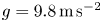$g = 9.8\,\textrm {m}\,\textrm {s}^{-2}$ and $h = 10$ m: (a) $\theta = 0$ (downstream); (b) $\theta = {\rm \pi}$ (upstream) and (c) $\theta = {\rm \pi}/2$ (orthogonal).

The squeezing of the interfacial wavefronts with decreasing $\alpha$ can be seen in figure 23(a). The effect is strengthened considerably when the density jump is smaller (i.e. when the interfacial waves are slower) which we achieve by decreasing $\rho _2$ from $1020$ to $1006\,\textrm {kg}\,\textrm {m}^{-3}$. The wavefronts are plotted in figure 23(b) for the same values of $\gamma$ and $\alpha$ as in figure 23(a). In all cases, $\gamma < {s}/{m(0)}$, i.e. there are no critical layers.