


1. Introduction
The existence of an interface between two fluid molecules or a fluid element and a solid substrate generates interfacial tension: a state function that depends on the temperature, fluid electric charge density and fluid composition, for example (Scriven Reference Scriven1960). Therefore, a variation of temperature, concentration, electric charge density, and so on, along an interface creates an interfacial tension gradient, which leads to Marangoni flow. If temperature fluctuations create a gradient in the interfacial tension, the phenomenon is called the thermocapillary effect or thermal Marangoni effect. Likewise, electro-capillarity, the solutal Marangoni effect, and so on, also exist depending on the genesis of the flow. Thermocapillary (TC) flow is noted to influence several practically relevant processes, such as in weld pools (Ramanan & Korpela Reference Ramanan and Korpela1990), in liquid combustion processes (Prokofiev & Smolyakov Reference Prokofiev and Smolyakov2019), during crystal growth (Cuvelier & Driessen Reference Cuvelier and Driessen1986), in droplet coalescence (Rother & Davis Reference Rother and Davis1999) and during bubble migration (Chen & Lee Reference Chen and Lee1992).
The thermal Marangoni effect is important for understanding and manipulating liquid–liquid systems. The constant formation of dimples on unevenly heated silicone-oil films (mean thickness varying from 0.125 to 1.684 mm) was experimentally studied and was reported to be due to the TC effect (Burelbach, Bankoff & Davis Reference Burelbach, Bankoff and Davis1990). Liu and Roux (Reference Liu and Roux1998) explored the TC flow in a molten B2O3-GaAs binary system, and Binghong et al. (Reference Binghong, Qiushen, Liang, Yonglong and Wenrui2002) studied TC flows in a two-layer binary system of paraffin and 2 FC-70 inclusive of air entrainment. During the IML2 mission of Spacelab aboard the US Space Shuttle, Georis et al. (Reference Georis, Hennenberg, Lebon and Legros1999) conducted microgravity experiments to examine the TC effect in a sandwiched liquid film (ternary-liquid) system. Alexeev, Roisman & Stephan (Reference Alexeev, Roisman and Stephan2005) and Fath et al. (Reference Fath, Horn, Roisman, Stephan and Bothe2015) explored the TC effect in a microchannel due to wall topology, both experimentally and numerically. Microscale particle image velocimetry is generally used to visualize the flow pattern within such systems (Amador et al. Reference Amador, Ren, Tabak, Alapan, Yasa and Sitti2019). These microfluidic devices exploiting the TC effect can be used for precision clinical assays at the point of care.
The Marangoni effect has also been studied mathematically owing to the rich physics it offers. Birikh (Reference Birikh1966) reported an exact solution for the TC convection of a planar horizontal liquid layer, for a constant temperature gradient at the boundaries. Sen and Davis (Reference Sen and Davis1982) theoretically explored the steady TC flow of liquid in a two-dimensional rectangular slot with a free top surface using the asymptotic approach. Tan, Bankoff & Davis (Reference Tan, Bankoff and Davis1990) employed the long-wave theory to study a thin liquid film's TC flow over a flat surface, subjected to the two-dimensional periodic (spatially varying) temperature distribution. Pendse & Esmaeeli (Reference Pendse and Esmaeeli2010) semi-analytically solved the Navier–Stokes and energy equations to explain the thermal Marangoni flow in a binary-liquid system. They considered a periodic thermal stimulus at the lower surface, while the upper surface was maintained at a uniform temperature.
The standard methodologies employed to obtain a theoretical solution for the flow dynamics at small scales are lubrication-theory-based models (Saprykin, Trevelyan, Koopmans, & Kalliadasis Reference Saprykin, Trevelyan, Koopmans and Kalliadasis2007; Frumkin & Oron Reference Frumkin and Oron2016; Pham, Cheng, & Kumar Reference Pham, Cheng and Kumar2017) and the asymptotic approach (Strani, Piva, & Graziani Reference Strani, Piva and Graziani1983; Chan, Chen & Mazumder Reference Chan, Chen and Mazumder1988). Numerous types of convections caused by buoyancy or the TC force have been effectively studied using asymptotic theory. Poulikakos & Bejan (Reference Poulikakos and Bejan1983) studied flows in an attic heated from below, while Cormack, Leal & Imberger (Reference Cormack, Leal and Imberger1974) considered buoyancy-driven flows in a rectangular container delimited by differently heated lateral walls.
Several past TC studies are mainly focused on instability analysis (Smith & Davis Reference Smith and Davis1983; Goussis & Kelly Reference Goussis and Kelly1990; Mercier & Normand Reference Mercier and Normand1996; Burguete Reference Burguete2001). Oron and Nepomnyashchy (Reference Oron and Nepomnyashchy2004) investigated the beginning of Marangoni instability in a binary-liquid system with a non-deformable interface under the influence of the Soret effect. Patne, Agnon & Oron (Reference Patne, Agnon and Oron2021) performed a stability analysis in a liquid layer with an imposed oblique temperature gradient. Thermal instability due to Bénard convection is also explored (Eckert, Bestehorn, & Thess Reference Eckert, Bestehorn and Thess1998; Tomita & Abe Reference Tomita and Abe2000; Schatz & Neitzel Reference Schatz and Neitzel2001). However, we assume low capillary number flow in the current study, which leads to a stable TC flow in the liquid layers with nearly flat interfaces.
Most of the theoretical analysis performed on TC assumes no-slip conditions at the walls (Pimputkar & Ostrach Reference Pimputkar and Ostrach1980; Liu & Roux Reference Liu and Roux1998; Pendse & Esmaeeli Reference Pendse and Esmaeeli2010; Agrawal, Das & Dhar Reference Agrawal, Das and Dhar2022). Although a few works are reported on the TC flow in microchannels with wall slip boundary conditions, they are primarily focused on the stability analysis of the system (Tiwari & Davis Reference Tiwari and Davis2014; Kowal, Davis, & Voorhees Reference Kowal, Davis and Voorhees2018; Chattopadhyay, Mukhopadhyay, Barua, & Gaonkar Reference Chattopadhyay, Mukhopadhyay, Barua and Gaonkar2021). Ghosh and Chakraborty (Reference Ghosh and Chakraborty2012) observed that the introduction of patterned wettability at the microchannel walls prompts mixing in an electroosmotic flow. Here, we explore the role of the interplay of the patterned wall wettability and the TC effect by the periodic wall thermal stimuli on the mixing dynamics.
Owing to the importance and controllability of the TC effect, we aim to harness its capabilities for fluidic actuation and solute transport in microscale fluid handling systems. This study theoretically explores the TC effect in a ternary-liquid system due to periodic wall thermal stimuli within a microchannel with patterned wall wettability. Such a system appears in certain modern technologies working with intricate multilayer systems. One such example is a crystal formation technique used in space laboratory missions called the liquid encapsulation crystal growth technique (Ratke, Walter & Feuerbacher Reference Ratke, Walter and Feuerbacher1996). This technique produces high quality crystals by sandwiching the melt between fluid layers. The present work aims to understand the interplay of the periodic thermal stimuli, wall wettability patterns and the fluids’ thermophysical properties in the system's mixing phenomenon. Given the importance of the mixing process and to obtain quick sample processing at small scales, numerous experimental, numerical and theoretical analyses have been performed to understand the TC-driven flow in multilayer systems (Nepomnyashchy & Simanovskii Reference Nepomnyashchy and Simanovskii1999; Shevtsova et al. Reference Shevtsova, Simanovskii, Nepomnyashchy and Legros2005; Simanovskii Reference Simanovskii2007). However, none of the earlier works address the role of surface wettability of the microchannel walls. Also, the past works on the TC effect in multilayer systems are restricted to directional temperature gradients, and do not consider periodic thermal boundary conditions on the confining walls, which justifies the novelty of the present work.
We solve the decoupled energy and Navier–Stokes equation for a ternary-liquid system by employing the perturbation method to obtain the temperature and the streamfunction distribution within the microchannel. The mathematical analyses are performed under the assumption of negligible Marangoni number and flat interfaces. Our study also confirms the credibility of the above assumptions by evaluating the Marangoni and the capillary numbers for the problem using the characteristic parameters. Further, we also obtain an estimated profile of the interfaces, which reveals that the interfacial deformation is negligible relative to the system length scales. Lastly, the transport of solute in the system is numerically explored.
2. Description of the physical system
Our study considers a ternary-liquid system which is sandwiched between the two parallel plates of a microchannel in microgravity conditions. The participating fluids are assumed to be immiscible with each other. A typical example of such a combination of fluids is mentioned in table 1. The bottom and the top walls are exposed to periodic thermal stimuli:  $\overline {{T_l}} (1 + {\delta _l}\cos (\alpha (\bar{x}/\overline {{l_c}} )) + \delta _l^2\cos (2\alpha (\bar{x}/\overline {{l_c}} )))$ and $ \overline {{T_u}} (1 + {\delta _u}\cos (\alpha (\bar{x}/\overline {{l_c}} ) + \theta ) + \delta _u^2\cos (2\alpha (\bar{x}/\overline {{l_c}} ) + 2\theta ))$, where $\overline {{T_l}} /\overline {{T_u}} $, $\overline {{l_c}} $, $\alpha $ and $\theta $ are the mean temperature, characteristic length scale and oscillation constants, and ${\delta _i}({\sim} O(0.1))$ is the perturbation parameter (here, $i = l\ \textrm{and}\ u$ represent the bottom and the top walls, respectively) (figure 1). Usually, any periodic function can be written as the summation of n harmonic terms using Fourier series, where n is an integer whose value tends to infinity. Inspired by the Fourier expansion, we have considered a temperature function up to the second harmonics. Although a few past works are reported to consider periodic wall temperature up to the first harmonic (Pendse & Esmaeeli Reference Pendse and Esmaeeli2010; Agrawal et al. Reference Agrawal, Das and Dhar2022), in this study we have deemed the second-harmonic function to illustrate how to accommodate for the higher-order terms. Further, the inclusion of the second harmonic in the thermal boundary condition is a mathematical requirement of the problem to incorporate the periodic behaviour of wall slip in the subsequent analysis. The symbols with an overhead bar represent the dimensional quantities and those without a bar are dimensionless quantities (normalized by their corresponding reference values) in the subsequent analysis.
Table 1. Details of immiscible ternary-liquid system.


Figure 1. The ternary-liquid layers in a micro-conduit with periodic thermal stimuli applied at the channel walls. Here, coordinate axes  $\bar{x}$ and $\bar{y}$ represent the axial and the lateral directions of the microchannel, respectively, and $\bar{a},\bar{b},\bar{c}$ denote the thicknesses of the fluid layers. The expressions for wall temperature and slip velocities are shown in the figure.
We consider patterned wettability at the walls, which creates slip boundary conditions as
 \begin{equation}{\bar{u}^a}{|_{\bar{y} ={-} (\bar{b}/2 + \bar{a})}} = \bar{\gamma }(\epsilon + {\delta _l}\cos (\alpha x)){\left. {\frac{{\partial {\bar{u}^a}}}{{\partial \bar{y}}}} \right|_{\bar{y} ={-} (\bar{b}/2 + \bar{a})}},\end{equation}
and
 \begin{equation}{\bar{u}^c}{|_{\bar{y} = (\bar{b}/2 + \bar{c})}} ={-} \bar{\gamma }(\epsilon + {\delta _u}\cos (\alpha x + \theta )){\left. {\frac{{\partial {\bar{u}^c}}}{{\partial \bar{y}}}} \right|_{\bar{y} = (\bar{b}/2 + \bar{c})}},\end{equation}
where  ${\bar{u}^a}$ and ${\bar{u}^c}$ are the velocity of the bottom and the top layers, respectively. $\bar{\gamma }$ and $\epsilon $ are slip parameters such that $\epsilon \ll {\delta _l}\ (\textrm{or}\ {\delta _u})$. Hence, $\bar{\gamma }{\delta _l}/\overline {{l_c}} $ and $\bar{\gamma }{\delta _u}/\overline {{l_c}} $ represent the normalized slip length $({l_s})$ at the bottom and the top walls, respectively. It is to be noted that the wall wettability patterns can be created independently of the wall temperature via chemical etching in practice. In the present analysis, we choose the wall slip to be in phase with the corresponding wall temperature for mathematical ease. Further, we have observed in our earlier work (Agrawal, Das & Dhar Reference Agrawal, Das and Dhar2023) that the influence of a periodic wavenumber and the phase of the wall slip is minimal compared with the slip length, the effect of which is discussed in detail in this paper (see § 4.3).
The mathematical analysis performed in the present work is based on two critical assumptions: (a) the governing non-dimensional numbers i.e. Reynolds number  $(Re = \overline {\rho V{l_c}} /\bar{\mu })$, capillary number $(Ca = \overline {\mu V} /\bar{\sigma })$ and Marangoni number $(Ma ={-} \overline {{\sigma _T}{l_c}\Delta T} /\overline {\mu {D_t}} \sim \overline {V{l_c}} /\overline {{D_t}} )$, as $\bar{V}\sim{-} \overline {{\sigma _T}\Delta T} /\bar{\mu }$ for TC flow (Pendse & Esmaeeli Reference Pendse and Esmaeeli2010), are much smaller than 1. Here, $\bar{\rho }$, $\bar{\mu }$, $\bar{\sigma }$, $\overline {{\sigma _T}} $ and $\overline {{D_t}} $ represent the fluid density, viscosity, surface tension coefficient, temperature coefficient of the surface tension and thermal diffusivity and $\bar{V}$, $\overline {{l_c}} $ and $\overline {\Delta T} $ are the characteristic velocity, length and temperature difference of the system. (b) The fluid–fluid interfaces remain undeformed and flat during the dynamics. The characteristic values of the problem's governing non-dimensional numbers can be determined using the typical values of the parameters. The usual orders of the length scale and the velocity in a microchannel are $10\ \mathrm{\mu }\textrm{m}$ and ${10^{ - 4}}\ \textrm{m}\ {\textrm{s}^{ - 1}}$, respectively (Das & Chakraborty Reference Das and Chakraborty2018). Taking the thermophysical properties of water at $300\ \textrm{K}$ ( $\bar{\rho } = 997\ \textrm{kg}\ {\textrm{m}^{ - 3}}$, $\bar{\mu } = 0.00086\ \textrm{Ns}\ {\textrm{m}^{ - 2}}$, $\bar{\sigma } = 0.072\ \textrm{N}\ {\textrm{m}^{ - 1}}$, $\overline {{D_t}} = 1.5 \times {10^{ - 7}}\ {\textrm{m}^2}\ {\textrm{s}^{ - 1}}$) (Bergman et al. Reference Bergman, Lavine, Incropera and Dewitt2011), the non-dimensional numbers can be evaluated as: $Re\sim {10^{ - 3}}$, $Ca\sim {10^{ - 6}}$ and $Ma\sim {10^{ - 3}}$. The credibility of the second assumption (flat and undeformed interfaces) is demonstrated by obtaining the estimated profiles of the deformed interfaces in a later part of the paper.
Further, we have assumed stable parallel flows in the three liquid layers as it is well established in the literature that an instability arises in a multilayer system only above a critical value of the Marangoni number  $(Ma)$, which is usually of the order of ${\sim} O({10^3})$. For instance, the stability analysis performed by Simanovskii (Reference Simanovskii2007) demonstrates that the critical value of the Marangoni number $(Ma)$ to incite instability is $Ma = 1250$ for a 47v2 silicone-oil–water–7v2 silicone-oil system, and $Ma = 450$ for an air–ethylene glycol–fluorinert FC75 system. Since the order of the Marangoni number in the present analysis is ${\sim} O({10^3})$, stable parallel flows can be comfortably considered.
3. Mathematical description of the system
3.1. Thermal transport analysis
We obtain the approximate analytical solution for the system by appealing to the asymptotic perturbation approach. We solve the energy equation in the limiting case of small Marangoni number (or Péclet number), which reduces the governing differential equation to the Laplacian of the temperature field, as
 \begin{equation}{\nabla
^2}{\bar{T}^i}(x,y) = 0,\quad \textrm{where}\ i = a,b,c\ \textrm{and}\ {\nabla ^2} = \frac{{{\partial ^2}}}{{\partial
{x^2}}} + \frac{{{\partial ^2}}}{{\partial
{y^2}}}.\end{equation}
\begin{equation}{\nabla
^2}{\bar{T}^i}(x,y) = 0,\quad \textrm{where}\ i = a,b,c\ \textrm{and}\ {\nabla ^2} = \frac{{{\partial ^2}}}{{\partial
{x^2}}} + \frac{{{\partial ^2}}}{{\partial
{y^2}}}.\end{equation}
Here,
 \begin{align}
{\bar{T}^i}(x,y) = \left\{{\begin{array}{@{}ll@{}} {{\bar{T}^a}(x,y); }&{ - a - \dfrac{b}{2} < y < - \dfrac{b}{2}}\\
{{\bar{T}^b}(x,y);}&{ - \dfrac{b}{2} < y < \dfrac{b}{2}}\\ {{\bar{T}^c}(x,y); }&{\dfrac{b}{2} <
y < \dfrac{b}{2} + c} \end{array}}\right.,\end{align}
\begin{align}
{\bar{T}^i}(x,y) = \left\{{\begin{array}{@{}ll@{}} {{\bar{T}^a}(x,y); }&{ - a - \dfrac{b}{2} < y < - \dfrac{b}{2}}\\
{{\bar{T}^b}(x,y);}&{ - \dfrac{b}{2} < y < \dfrac{b}{2}}\\ {{\bar{T}^c}(x,y); }&{\dfrac{b}{2} <
y < \dfrac{b}{2} + c} \end{array}}\right.,\end{align}
where a, b and c represent the properties of the lower, the middle and the upper liquid layers, respectively. Boundary conditions available to solve the above partial differential equation (3.1) are:
(a) Bottom wall surface temperature
(3.3) \begin{equation}{\bar{T}^a}{|_{y ={-} (b/2 + a)}} = \overline {{T_l}} (1 + {\delta _l}\cos (\alpha x) + \delta _l^2\cos (2\alpha x)).\end{equation}
(b) Top wall surface temperature
(3.4)\begin{equation}{\bar{T}^c}{|_{y = (b/2 + c)}} = \overline {{T_u}} (1 + {\delta _u}\cos (\alpha x + \theta ) + \delta _u^2\cos (2\alpha x + 2\theta )).\end{equation}(c) Temperature at the separating interface between fluid ‘
$a$’ and fluid ‘$b$’
(3.5)\begin{equation}{\bar{T}^a}{|_{y ={-} b/2}} = {\bar{T}^b}{|_{y ={-} b/2}}.\end{equation}(d) Temperature at the separating interface between fluid ‘
$b$’ and fluid ‘$c$’
(3.6)\begin{equation}{ {{\bar{T}^b}} |_{y = b/2}} = { {{\bar{T}^c}} |_{y = b/2}}.\end{equation}(e) Heat flux across the separating interface between fluid ‘
$a$’ and fluid ‘$b$’
(3.7)\begin{equation}{\bar{\lambda }^a}{\left. {\frac{{\partial {\bar{T}^a}}}{{\partial y}}} \right|_{y ={-} b/2}} = {\bar{\lambda }^b}{\left. {\frac{{\partial {\bar{T}^b}}}{{\partial y}}} \right|_{y ={-} b/2}}.\end{equation}(f ) Heat flux across the separating interface between fluid ‘
$b$’ and fluid ‘$c$’
(3.8)\begin{equation}{\bar{\lambda }^b}{\left. {\frac{{\partial {\bar{T}^b}}}{{\partial y}}} \right|_{y = b/2}} = {\bar{\lambda }^c}{\left. {\frac{{\partial {\bar{T}^c}}}{{\partial y}}} \right|_{y = b/2}}.\end{equation}


Here,  ${\bar{\lambda }^i}$ represents the thermal conductivity of fluid ‘ $i$’. We solve the required partial differential equation (2.1) to obtain the temperature distribution within the microchannel by an asymptotic approach using the perturbation method, as
 \begin{equation}{\bar{T}^i} = \bar{T}_0^i + {\delta _l}\bar{T}_1^i + {\delta _u}\bar{T}_2^i + {\delta _l}{\delta _u}\bar{T}_3^i + {\delta _l}^2\bar{T}_4^i + {\delta}_u^2\bar{T}_5^i,\quad \textrm{where}\ i = a,b,c.\end{equation}
Now, the governing equation for each term can be written as
 \begin{equation}{\nabla ^2}\bar{T}_j^i(x,y) = 0;\quad \textrm{where}\ i = a,b,c;j = 0\unicode{x2013} 5;\quad \textrm{and}\quad {\nabla ^2} = \frac{{{\partial ^2}}}{{\partial {x^2}}} + \frac{{{\partial ^2}}}{{\partial {y^2}}}.\end{equation}
The modified boundary conditions are summarized in table 2.
Table 2. Modified boundary conditions for the temperature field.

A close observation of the boundary conditions mentioned in table 2 reveals that the zeroth-order term of the temperature field is a function of ‘y’  $(\bar{T}_0^i(\kern0.7pt y))$ and is obtained by solving the second-order ordinary differential equation $({\textrm{d}^2}\bar{T}_0^i(\kern0.7pt y)/\textrm{d}{y^2} = 0)$, which gives
 \begin{align}
\bar{T}_0^i(\kern0.7pt y) = \left\{
\begin{aligned}
\bar{T}_0^a(\kern0.7pt y) &= \dfrac{{({{\bar{T}}_u} - {{\bar{T}}_l})y}}{{c\!\left( {\dfrac{{{\lambda_a}}}{{{\lambda_c}}}} \right) + b\!\left( {\dfrac{{{\lambda_a}}}{{{\lambda_b}}}} \right) + a}}\notag\\
&\quad + \dfrac{{2{{\bar{T}}_l}c\!\left( {\dfrac{{{\lambda_a}}}{{{\lambda_c}}}} \right) +
2{{\bar{T}}_l}b\!\left( {\dfrac{{{\lambda_a}}}{{{\lambda_b}}}} \right) - {{\bar{T}}_l}b + 2{{\bar{T}}_u}a + {{\bar{T}}_u}b}}{{2\left( {c\!\left(
{\dfrac{{{\lambda_a}}}{{{\lambda_c}}}} \right) + b\!\left( {\dfrac{{{\lambda_a}}}{{{\lambda_b}}}} \right) + a} \right)}},\quad
- a - \dfrac{b}{2} < y < - \dfrac{b}{2}\notag\\
\bar{T}_0^b(\kern0.7pt y) &= \dfrac{{({{\bar{T}}_u} -
{{\bar{T}}_l})\left( {\dfrac{{{\lambda_a}}}{{{\lambda_b}}}}
\right)y}}{{c\!\left( {\dfrac{{{\lambda_a}}}{{{\lambda_c}}}}
\right) + b\!\left( {\dfrac{{{\lambda_a}}}{{{\lambda_b}}}}
\right) + a}}\notag\\ &\quad + \dfrac{{2{{\bar{T}}_l}c\!\left(
{\dfrac{{{\lambda_a}}}{{{\lambda_c}}}} \right) +
{{\bar{T}}_l}b\!\left( {\dfrac{{{\lambda_a}}}{{{\lambda_b}}}}
\right) + {{\bar{T}}_u}b\!\left(
{\dfrac{{{\lambda_a}}}{{{\lambda_b}}}} \right) +
2{{\bar{T}}_u}a}}{{2\left( {c\!\left(
{\dfrac{{{\lambda_a}}}{{{\lambda_c}}}} \right) + b\!\left(
{\dfrac{{{\lambda_a}}}{{{\lambda_b}}}} \right) + a}
\right)}},\quad - \dfrac{b}{2} < y < \dfrac{b}{2}\notag\\
\bar{T}_0^c(\kern0.7pt y) &= \dfrac{{({{\bar{T}}_u} -
{{\bar{T}}_l})\left( {\dfrac{{{\lambda_a}}}{{{\lambda_c}}}}
\right)y}}{{c\!\left( {\dfrac{{{\lambda_a}}}{{{\lambda_c}}}}
\right) + b\!\left( {\dfrac{{{\lambda_a}}}{{{\lambda_b}}}}
\right) + a}}\notag\\ &\quad + \dfrac{{{{\bar{T}}_l}b\!\left(
{\dfrac{{{\lambda_a}}}{{{\lambda_c}}}} \right) +
2{{\bar{T}}_l}c\!\left(
{\dfrac{{{\lambda_a}}}{{{\lambda_c}}}} \right) -
{{\bar{T}}_u}b\!\left( {\dfrac{{{\lambda_a}}}{{{\lambda_c}}}}
\right) + 2{{\bar{T}}_u}b\!\left(
{\dfrac{{{\lambda_a}}}{{{\lambda_b}}}} \right) +
2{{\bar{T}}_u}a}}{{2\left( {c\!\left(
{\dfrac{{{\lambda_a}}}{{{\lambda_c}}}} \right) + b\!\left(
{\dfrac{{{\lambda_a}}}{{{\lambda_b}}}} \right) + a}
\right)}},\quad\dfrac{b}{2} < y < \dfrac{b}{2} + c.
\end{aligned} \right.\end{align}
\begin{align}
\bar{T}_0^i(\kern0.7pt y) = \left\{
\begin{aligned}
\bar{T}_0^a(\kern0.7pt y) &= \dfrac{{({{\bar{T}}_u} - {{\bar{T}}_l})y}}{{c\!\left( {\dfrac{{{\lambda_a}}}{{{\lambda_c}}}} \right) + b\!\left( {\dfrac{{{\lambda_a}}}{{{\lambda_b}}}} \right) + a}}\notag\\
&\quad + \dfrac{{2{{\bar{T}}_l}c\!\left( {\dfrac{{{\lambda_a}}}{{{\lambda_c}}}} \right) +
2{{\bar{T}}_l}b\!\left( {\dfrac{{{\lambda_a}}}{{{\lambda_b}}}} \right) - {{\bar{T}}_l}b + 2{{\bar{T}}_u}a + {{\bar{T}}_u}b}}{{2\left( {c\!\left(
{\dfrac{{{\lambda_a}}}{{{\lambda_c}}}} \right) + b\!\left( {\dfrac{{{\lambda_a}}}{{{\lambda_b}}}} \right) + a} \right)}},\quad
- a - \dfrac{b}{2} < y < - \dfrac{b}{2}\notag\\
\bar{T}_0^b(\kern0.7pt y) &= \dfrac{{({{\bar{T}}_u} -
{{\bar{T}}_l})\left( {\dfrac{{{\lambda_a}}}{{{\lambda_b}}}}
\right)y}}{{c\!\left( {\dfrac{{{\lambda_a}}}{{{\lambda_c}}}}
\right) + b\!\left( {\dfrac{{{\lambda_a}}}{{{\lambda_b}}}}
\right) + a}}\notag\\ &\quad + \dfrac{{2{{\bar{T}}_l}c\!\left(
{\dfrac{{{\lambda_a}}}{{{\lambda_c}}}} \right) +
{{\bar{T}}_l}b\!\left( {\dfrac{{{\lambda_a}}}{{{\lambda_b}}}}
\right) + {{\bar{T}}_u}b\!\left(
{\dfrac{{{\lambda_a}}}{{{\lambda_b}}}} \right) +
2{{\bar{T}}_u}a}}{{2\left( {c\!\left(
{\dfrac{{{\lambda_a}}}{{{\lambda_c}}}} \right) + b\!\left(
{\dfrac{{{\lambda_a}}}{{{\lambda_b}}}} \right) + a}
\right)}},\quad - \dfrac{b}{2} < y < \dfrac{b}{2}\notag\\
\bar{T}_0^c(\kern0.7pt y) &= \dfrac{{({{\bar{T}}_u} -
{{\bar{T}}_l})\left( {\dfrac{{{\lambda_a}}}{{{\lambda_c}}}}
\right)y}}{{c\!\left( {\dfrac{{{\lambda_a}}}{{{\lambda_c}}}}
\right) + b\!\left( {\dfrac{{{\lambda_a}}}{{{\lambda_b}}}}
\right) + a}}\notag\\ &\quad + \dfrac{{{{\bar{T}}_l}b\!\left(
{\dfrac{{{\lambda_a}}}{{{\lambda_c}}}} \right) +
2{{\bar{T}}_l}c\!\left(
{\dfrac{{{\lambda_a}}}{{{\lambda_c}}}} \right) -
{{\bar{T}}_u}b\!\left( {\dfrac{{{\lambda_a}}}{{{\lambda_c}}}}
\right) + 2{{\bar{T}}_u}b\!\left(
{\dfrac{{{\lambda_a}}}{{{\lambda_b}}}} \right) +
2{{\bar{T}}_u}a}}{{2\left( {c\!\left(
{\dfrac{{{\lambda_a}}}{{{\lambda_c}}}} \right) + b\!\left(
{\dfrac{{{\lambda_a}}}{{{\lambda_b}}}} \right) + a}
\right)}},\quad\dfrac{b}{2} < y < \dfrac{b}{2} + c.
\end{aligned} \right.\end{align}
Using the variable separation approach to replace  $\bar{T}_j^i(x,y) = X_j^i(x)Y_j^i(\kern0.7pt y)$ in (3.10) for the higher-order terms of the temperature field and noticing the periodicity of the temperature boundary conditions along the axial direction, we obtain
 \begin{gather}\frac{{{\textrm{d}^2}Y_j^i(\kern0.7pt y)}}{{\textrm{d}{y^2}}}
- n_j^{{i^2}}Y_j^i(\kern0.7pt y) = 0\quad \textrm{and}\quad
\frac{{{\textrm{d}^2}X_j^i(x)}}{{\textrm{d}\kern 0.06em {x^2}}} +
n_j^{{i^2}}X_j^i(x) =
0,\end{gather}
\begin{gather}\frac{{{\textrm{d}^2}Y_j^i(\kern0.7pt y)}}{{\textrm{d}{y^2}}}
- n_j^{{i^2}}Y_j^i(\kern0.7pt y) = 0\quad \textrm{and}\quad
\frac{{{\textrm{d}^2}X_j^i(x)}}{{\textrm{d}\kern 0.06em {x^2}}} +
n_j^{{i^2}}X_j^i(x) =
0,\end{gather}
 \begin{gather}\textrm{i}\textrm{.e}\textrm{.}\ Y_j^i(\kern0.7pt y)
= \bar{A}_j^i\cosh (n_j^iy) + \bar{B}_j^i\sinh
(n_j^iy)\quad \textrm{and}\quad X_j^i(x) = \bar{C}_j^i\cos
(n_j^ix) + \bar{D}_j^i\sin (n_j^ix),\end{gather}
\begin{gather}\textrm{i}\textrm{.e}\textrm{.}\ Y_j^i(\kern0.7pt y)
= \bar{A}_j^i\cosh (n_j^iy) + \bar{B}_j^i\sinh
(n_j^iy)\quad \textrm{and}\quad X_j^i(x) = \bar{C}_j^i\cos
(n_j^ix) + \bar{D}_j^i\sin (n_j^ix),\end{gather}
 \begin{gather}\textrm{i}\textrm{.e}\textrm{.}\ \bar{T}_j^i(x,y) = (\bar{A}_j^i\cosh (n_j^iy) + \bar{B}_j^i\sinh (n_j^iy))(\bar{C}_j^i\cos (n_j^ix) + \bar{D}_j^i\sin (n_j^ix)).\end{gather}
Here,  $\bar{A}_j^i,B_j^i,C_j^i,\bar{D}_j^i\ \textrm{and}\ n_j^i$ are arbitrary constants. By comparing the wall temperatures, evaluated by the general formula derived above (3.14) with the applied thermal stimuli, the general expressions for the temperature terms can be simplified, as mentioned in table 3.
Table 3. Expressions for different terms of the temperature field.

The values of the constants  $A_j^i$ and $B_j^i$, where $i = a,b,c\ \textrm{and}\ j = 1\unicode{x2013} 5$, are determined by applying the boundary conditions mentioned in table 2. The expressions of the constants obtained are intricated functions of the characteristic parameters and, hence, are not provided here to maintain the brevity of the paper. However, the behaviour of the temperature field and its dependence on different parameters are presented in § 4.1.
3.2. Hydrodynamic analysis
The temperature field obtained in the previous section clearly indicates the existence of interfacial temperature gradients along both the separating interfaces. We also know that the interfacial surface tensions are strong and inverse functions of the temperature (Kou et al. Reference Kou, Li, Zhang, Xu, Zhang, Shao, Ma, Deng and Li2019). The variation in the surface tension thus produced acts as a driving force to create periodic circulations (TC flow) of the participating fluids in the microchannel. We solve the continuity and the Navier–Stokes equations under the creeping flow assumption to obtain the flow characteristics of the TC flow, which are given as
 \begin{equation}\bar{\nabla}{\bar{\boldsymbol{u}}^i} = 0\quad \textrm{and}\quad - \bar{\nabla }{\bar{p}^i} + {\bar{\mu }^i}{\bar{\nabla }^2}{\bar{\boldsymbol{u}}^i} = 0,\quad \textrm{where}\ i = a,b,c.\end{equation}
Here,  ${\bar{\boldsymbol{u}}^i},{\bar{p}^i}\ \textrm{and}\ {\bar{\mu }^i}$ represent the velocity field, the pressure distribution and the fluid's dynamic viscosity. The above two equations (3.15) can be merged into a single governing equation by introducing the streamfunction $({\bar{\psi }^i}(x,y))$, which is defined as
 \begin{equation}{\bar{u}^i} = \frac{{\partial {\bar{\psi }^i}(x,y)}}{{\overline {{l_c}} \partial y}}\quad \textrm{and}\quad {\bar{v}^i} ={-} \frac{{\partial {\bar{\psi }^i}(x,y)}}{{\overline {{l_c}} \partial x}},\quad \textrm{where}\ i = a,b,c.\end{equation}
Here,  ${\bar{u}^i}$ and ${\bar{v}^i}$ are the horizontal and the vertical component of the velocity of the fluid ‘ $i$’. The existence of the streamfunction identically satisfies the continuity equation. Now, by substituting the velocities as a function of the streamfunction in the Navier–Stokes equation and taking the curl of the whole equation, we obtain
 \begin{equation}{\nabla ^4}{\bar{\psi }^i}(x,y) = \frac{{{\partial ^4}{\bar{\psi }^i}(x,y)}}{{\partial {x^4}}} + 2\frac{{{\partial ^4}{\bar{\psi }^i}(x,y)}}{{\partial {x^2}\partial {y^2}}} + \frac{{{\partial ^4}{\bar{\psi }^i}(x,y)}}{{\partial {y^4}}} = 0,\quad \textrm{where}\ i = a,b,c.\end{equation}
Here,
 \begin{equation}
{\bar{\psi }^i}(x,y) = \left\{{\begin{array}{@{}ll@{}}
{{\bar{\psi }^a}(x,y),}&{- a - \dfrac{b}{2} < y < - \dfrac{b}{2}}\\
{{\bar{\psi }^b}(x,y), }&{ - \dfrac{b}{2} < y < \dfrac{b}{2}}\\
{{\bar{\psi }^c}(x,y),}&{\dfrac{b}{2} < y <
\dfrac{b}{2} + c} \end{array}}
\right..\end{equation}
\begin{equation}
{\bar{\psi }^i}(x,y) = \left\{{\begin{array}{@{}ll@{}}
{{\bar{\psi }^a}(x,y),}&{- a - \dfrac{b}{2} < y < - \dfrac{b}{2}}\\
{{\bar{\psi }^b}(x,y), }&{ - \dfrac{b}{2} < y < \dfrac{b}{2}}\\
{{\bar{\psi }^c}(x,y),}&{\dfrac{b}{2} < y <
\dfrac{b}{2} + c} \end{array}}
\right..\end{equation}
The governing equation for the streamfunction (3.17) is constrained to the boundary conditions mentioned below:
(a) Wall slip velocities
(3.19a)\begin{gather}{\left. {\frac{{\partial {\bar{\psi }^a}(x,y)}}{{\partial y}}} \right|_{y ={-} (b/2 + a)}} = \gamma (\epsilon + {\delta _l}\cos (\alpha x)){\left. {\frac{{{\partial^2}{\bar{\psi }^a}(x,y)}}{{\partial {y^2}}}} \right|_{y ={-} (b/2 + a)}},\end{gather}(3.19b)\begin{gather}{\left. {\frac{{\partial {\bar{\psi }^c}(x,y)}}{{\partial y}}} \right|_{y = (b/2 + c)}} ={-} \gamma (\epsilon + {\delta _u}\cos (\alpha x + \theta )){\left. {\frac{{{\partial^2}{\bar{\psi }^c}(x,y)}}{{\partial {y^2}}}} \right|_{y = (b/2 + c)}}.\end{gather}(b) No-penetration boundary condition across the walls
(3.20)\begin{equation}{\left. {\frac{{\partial {\bar{\psi }^a}(x,y)}}{{\partial x}}} \right|_{y ={-} (b/2 + a)}} = {\left. {\frac{{\partial {\bar{\psi }^c}(x,y)}}{{\partial x}}} \right|_{y = (b/2 + a)}} = 0.\end{equation}(c) No-slip boundary condition at the fluid-fluid interfaces
(3.21a,b)\begin{align}{\left. {\frac{{\partial {\bar{\psi }^a}(x,y)}}{{\partial y}}} \right|_{y ={-} b/2}} = {\left. {\frac{{\partial {\bar{\psi }^b}(x,y)}}{{\partial y}}} \right|_{y ={-} b/2}}\quad \textrm{and}\quad {\left. {\frac{{\partial {\bar{\psi }^b}(x,y)}}{{\partial y}}} \right|_{y = b/2}} = {\left. {\frac{{\partial {\bar{\psi }^c}(x,y)}}{{\partial y}}} \right|_{y = b/2}}.\end{align}(d) No-penetration boundary condition at the fluid-fluid interfaces
(3.22a,b)\begin{align}{\left. {\frac{{\partial {\bar{\psi }^a}(x,y)}}{{\partial x}}} \right|_{y ={-} b/2}} = {\left. {\frac{{\partial {\bar{\psi }^b}(x,y)}}{{\partial x}}} \right|_{y ={-} b/2}} = 0\quad \textrm{and}\quad {\left. {\frac{{\partial {\bar{\psi }^b}(x,y)}}{{\partial x}}} \right|_{y = b/2}} = {\left. {\frac{{\partial {\bar{\psi }^c}(x,y)}}{{\partial x}}} \right|_{y = b/2}} = 0.\end{align}(e) Shear stress balance at the interfaces
(3.23a)\begin{gather}{\left. {{\bar{\mu }^a}\left( {\frac{{{\partial^2}{\bar{\psi }^a}}}{{\partial {y^2}}} - \frac{{{\partial^2}{\bar{\psi }^a}}}{{\partial {x^2}}}} \right)} \right|_{y ={-} b/2}} - {\left. {{\bar{\mu }^b}\left( {\frac{{{\partial^2}{\bar{\psi }^b}}}{{\partial {y^2}}} - \frac{{{\partial^2}{\bar{\psi }^b}}}{{\partial {x^2}}}} \right)} \right|_{y ={-} b/2}} = \overline {{\sigma _T}{l_c}} {\left. {\frac{{\partial \bar{T}}}{{\partial x}}} \right|_{y ={-} b/2}},\end{gather}(3.23b)We obtain the solution for the streamfunction by the perturbation method, assuming\begin{gather}{\left. {{\bar{\mu }^b}\left( {\frac{{{\partial^2}{\bar{\psi }^b}}}{{\partial {y^2}}} - \frac{{{\partial^2}{\bar{\psi }^b}}}{{\partial {x^2}}}} \right)} \right|_{y = b/2}} - {\left. {{\bar{\mu }^c}\left( {\frac{{{\partial^2}{\bar{\psi }^c}}}{{\partial {y^2}}} - \frac{{{\partial^2}{\bar{\psi }^c}}}{{\partial {x^2}}}} \right)} \right|_{y = b/2}} = \overline {{\sigma _T}{l_c}} {\left. {\frac{{\partial \bar{T}}}{{\partial x}}} \right|_{y = b/2}}.\end{gather}(3.24)\begin{equation}{\bar{\psi }^i} = {\delta _l}\bar{\psi }_1^i + {\delta _u}\bar{\psi }_2^i + {\delta _l}{\delta _u}\bar{\psi }_3^i + {\delta _l}^2\bar{\psi }_4^i + {\delta _u^2}\bar{\psi }_5^i,\quad \textrm{where}\ i = a,b,c.\end{equation}


By observing the boundary conditions, we choose approximate forms for the different terms of the streamfunction, as mentioned in table 4. The governing differential equations for each term of the series expansion of the streamfunction (3.24) are mentioned in table 5 and the corresponding boundary conditions are provided in the Appendix (see tables 7 and 8). The term-wise boundary conditions are obtained by substituting the general form of each term in ((3.19)–(3.23)) and then comparing the coefficients of the perturbation parameters.
Table 4. General forms for the different terms of the streamfunction.

Table 5. The term-wise governing differential equations of the streamfunction.

The general solution for  $g_j^i(\kern0.7pt y),\ \textrm{where}\ i = a,b,c\ \textrm{and}\ j = 1\unicode{x2013} 5$, is obtained by choosing $g_j^i(\kern0.7pt y) = {e^{q_j^iy}}$ to convert the governing differential equation into its characteristic form, as
 \begin{align}q_j^{{i^4}} - 2{\alpha ^2}q_j^{{i^2}} + {\alpha ^4} &= 0,\quad \textrm{where}\ i = a,b,c\ \textrm{and}\ j = 1,2,\end{align}
 \begin{align}q_j^{{i^4}} - 8{\alpha ^2}q_j^{{i^2}} + 16{\alpha ^4} &= 0,\quad \textrm{where}\ i = a,b,c\ \textrm{and}\ j = 3\unicode{x2013} 5,\end{align}
which gives  ${(q_j^{{i^2}} - {\alpha ^2})^2} = 0$ or $q_j^i ={\pm} \alpha $ for $j = 1, 2$ and ${(q_j^{{i^2}} - 4{\alpha ^2})^2} = 0$ or $q_j^i ={\pm} 2\alpha \ \textrm{for}\ j = 3\unicode{x2013} 5$. Therefore, the general solution of the above biharmonic equation (3.24) is given by
 \begin{equation}g_j^i(\kern0.7pt y) = (P_j^i + Q_j^iy)\cosh (m\alpha y) + (R_j^i + S_j^iy)\sinh (m\alpha y),\quad \textrm{where}\ i = a,b,c.\end{equation}
Here,  $m = 1$ for $j = 1, 2$ and $m = 2$ for $j = 3\unicode{x2013} 5$. We assume the general form of $h_j^i(\kern0.7pt y)$ to be $E_j^iy + F_j^i{y^2}$, as adopted by Ghosh and Chakraborty (Reference Ghosh and Chakraborty2012) in an allied problem. The constants $P_j^i,Q_j^i,R_j^i,S_j^i,E_j^i\ \textrm{and}\ F_j^i$ are determined by appealing to the boundary conditions mentioned in the Appendix (tables 7 and 8). The expressions of the constants are involved functions of the parameters and, hence, are not provided in the manuscript to maintain its brevity. However, the dependences of the streamfunction (or the flow velocity) on different parameters are discussed in detail in § 4.2.
3.3. Interface deformation dynamics
The asymptotic solutions obtained in the previous sections are valid for small governing non-dimensional numbers  $(Ma,Re\ \textrm{and}\ Ca)$ and flat (or undeformed) fluid–fluid interfaces. The credibility of the first assumption $(\textrm{i}\textrm{.e}\textrm{.}\ \textrm{negligible}\ Ma,Re\ \textrm{and}\ Ca)$ is discussed in § 2. Even though the small magnitude of Ca guarantees that the extent of deformations occurring in the interfaces is negligible, we obtain the deformed profiles of the two fluid–fluid interfaces using the results for the hydrodynamic characteristics to support the assumption of flat and undeformed interfaces. Knowing the velocity field in the microchannel, the deformation of the interfaces can be estimated by using the normal stress balance across the interfaces, as
 \begin{equation}(({\overline {{\tau _{yy}}} ^a} - {\overline {{\tau _{yy}}} ^b}) - ({\bar{p}^a} - {\bar{p}^b})){|_{y ={-} b/2}} = \overline {{\sigma _l}{\kappa _l}} ,\end{equation}
and
 \begin{equation}(({\overline {{\tau _{yy}}} ^b} - {\overline {{\tau _{yy}}} ^c}) - ({\bar{p}^b} - {\bar{p}^c})){|_{y = b/2}} = \overline {{\sigma _u}{\kappa _u}} ,\end{equation}
where  $\overline {{\tau _{yy}}} ={-} 2\bar{\mu }({\partial ^2}\bar{\psi }(x,y)/\partial \bar{x}\partial \bar{y})$ is the normal stress, $\bar{p}$ the pressure distribution, $\overline {{\sigma _l}} /\overline {{\sigma _u}} $ the surface tension coefficient at the lower/upper interfaces and $\overline {{\kappa _l}} /\overline {{\kappa _u}} $ the local curvature of the deformed interfaces; $\bar{\kappa }$ is defined such that it is positive for the case where the centre of curvatures of the interfaces falls below them and is given by
 \begin{equation}{\bar{\kappa }_i} = \frac{{\dfrac{{{\textrm{d}^2}{{\bar{y}}_i}}}{{\textrm{d}{\bar{x}^2}}}}}{{{{\left( {1 + {{\left( {\dfrac{{\textrm{d}{{\bar{y}}_i}}}{{\textrm{d}\kern0.06em \bar{x}}}} \right)}^2}} \right)}^{3/2}}}}\sim \frac{{{\textrm{d}^2}{{\bar{y}}_i}}}{{\textrm{d}{\bar{x}^2}}}\sim \frac{1}{{{{\bar{l}}_c}}}\frac{{{\textrm{d}^2}{y_i}}}{{\textrm{d}\kern 0.06em {x^2}}},\quad \textrm{where}\ i = l,u.\end{equation}
Here,  ${\bar{y}_i}$ is the vertical displacement of the interfaces relative to their initial undeformed position, and $l/u$ denotes the lower/upper interface. It is also discussed in the literature (Pendse & Esmaeeli Reference Pendse and Esmaeeli2010) that, for $Ca \ll 1$, the interfacial deformation is small enough to assume $(1 + {(\textrm{d}{\bar{y}_i}/\textrm{d}\kern0.06em \bar{x})^2})\sim 1$.
The extended expression of the normal stress  $(\overline {{\tau _{yy}}} )$ is given by
 \begin{equation}{\overline {{\tau _{yy}}} ^i} = \overline {{\tau _{yy}}} _1^i{\delta _l} + \overline {{\tau _{yy}}} _2^i{\delta _u} + \overline {{\tau _{yy}}} _3^i{\delta _l}{\delta _u} + \overline {{\tau _{yy}}} _4^i\delta _l^2 + \overline {{\tau _{yy}}} _5^i\delta _u^2,\quad \textrm{where}\ i = a,b,c.\end{equation}
Here, the different terms of the asymptotic series of the normal stress can be represented as
 \begin{align} & {\begin{bmatrix} {\dfrac{{\overline {{\tau_{yy}}}_1^i}}{{\cos (\alpha x)}}}\\
{\dfrac{{\overline {{\tau_{yy}}}_2^i}}{{\cos (\alpha x +
\theta )}}}\\ {\dfrac{{\overline {{\tau_{yy}}}_3^i}}{{4\cos
(2\alpha x + \theta )}}}\\ {\dfrac{{\overline
{{\tau_{yy}}}_4^i}}{{4\cos (2\alpha x)}}}\\
{\dfrac{{\overline {{\tau_{yy}}}_5^i}}{{4\cos (2\alpha x +
2\theta )}}} \end{bmatrix}} \nonumber\\ & \quad ={-}
\frac{{2{\bar{\mu}^i}\alpha }}{{{{\overline {{l_c}}
}^2}}}\begin{bmatrix} {(S_1^iy +
R_1^i)\alpha + Q_1^i} & {(Q_1^iy + P_1^i)\alpha +
S_1^i} & 0 & 0\\ {(S_2^iy + R_2^i)\alpha + Q_2^i} & {(Q_2^iy +
P_2^i)\alpha + S_2^i} & 0 & 0\\ 0 & 0 & {(S_3^iy + R_3^i)\alpha +
\dfrac{{Q_3^i}}{2}} & {(Q_3^iy + P_3^i)\alpha +
\dfrac{{S_3^i}}{2}}\\ 0 & 0 & {(S_4^iy + R_4^i)\alpha +
\dfrac{{Q_4^i}}{2}} & {(Q_4^iy + P_4^i)\alpha +
\dfrac{{S_4^i}}{2}}\\ 0 & 0 & {(S_5^iy + R_5^i)\alpha +
\dfrac{{Q_5^i}}{2}} & {(Q_5^iy + P_5^i)\alpha +
\dfrac{{S_5^i}}{2}} \end{bmatrix}\nonumber\\ & \qquad\times \begin{bmatrix}
{\cosh (\alpha y)}\\ {\sinh
(\alpha y)}\\ {\cosh (2\alpha y)}\\ {\sinh (2\alpha y)}
\end{bmatrix}.
\end{align}
\begin{align} & {\begin{bmatrix} {\dfrac{{\overline {{\tau_{yy}}}_1^i}}{{\cos (\alpha x)}}}\\
{\dfrac{{\overline {{\tau_{yy}}}_2^i}}{{\cos (\alpha x +
\theta )}}}\\ {\dfrac{{\overline {{\tau_{yy}}}_3^i}}{{4\cos
(2\alpha x + \theta )}}}\\ {\dfrac{{\overline
{{\tau_{yy}}}_4^i}}{{4\cos (2\alpha x)}}}\\
{\dfrac{{\overline {{\tau_{yy}}}_5^i}}{{4\cos (2\alpha x +
2\theta )}}} \end{bmatrix}} \nonumber\\ & \quad ={-}
\frac{{2{\bar{\mu}^i}\alpha }}{{{{\overline {{l_c}}
}^2}}}\begin{bmatrix} {(S_1^iy +
R_1^i)\alpha + Q_1^i} & {(Q_1^iy + P_1^i)\alpha +
S_1^i} & 0 & 0\\ {(S_2^iy + R_2^i)\alpha + Q_2^i} & {(Q_2^iy +
P_2^i)\alpha + S_2^i} & 0 & 0\\ 0 & 0 & {(S_3^iy + R_3^i)\alpha +
\dfrac{{Q_3^i}}{2}} & {(Q_3^iy + P_3^i)\alpha +
\dfrac{{S_3^i}}{2}}\\ 0 & 0 & {(S_4^iy + R_4^i)\alpha +
\dfrac{{Q_4^i}}{2}} & {(Q_4^iy + P_4^i)\alpha +
\dfrac{{S_4^i}}{2}}\\ 0 & 0 & {(S_5^iy + R_5^i)\alpha +
\dfrac{{Q_5^i}}{2}} & {(Q_5^iy + P_5^i)\alpha +
\dfrac{{S_5^i}}{2}} \end{bmatrix}\nonumber\\ & \qquad\times \begin{bmatrix}
{\cosh (\alpha y)}\\ {\sinh
(\alpha y)}\\ {\cosh (2\alpha y)}\\ {\sinh (2\alpha y)}
\end{bmatrix}.
\end{align}
The constants  $P_j^i,Q_j^i,R_j^i\ \textrm{and}\ S_j^i$ are as defined for the streamfunction, where $i = a,b,c$ and $j = 1\unicode{x2013} 5$. Further, the pressure distribution is obtained by partially integrating the $x\ \textrm{and}\ y$ momentum equations (3.15) and combining the results. The final expression of the pressure distribution in the microchannel is given by
 \begin{equation}{\bar{p}^i} = \bar{p}_1^i{\delta _l} + \bar{p}_2^i{\delta _u} + \bar{p}_3^i{\delta _l}{\delta _u} + \bar{p}_4^i\delta _l^2 + \bar{p}_5^i\delta _u^2,\quad \textrm{where}\ i = a,b,c.\end{equation}
Here, the different terms of the asymptotic series of the pressure distribution can be represented as
 \begin{align} &\begin{bmatrix} {\dfrac{{\bar{p}_1^i}}{{\cos
(\alpha x)}}}\\ {\dfrac{{\bar{p}_2^i}}{{\cos (\alpha x +
\theta )}}}\\ {\dfrac{{\bar{p}_3^i}}{{2\cos (2\alpha x +
\theta )}}}\\ {\dfrac{{\bar{p}_4^i}}{{2\cos (2\alpha
x)}}}\\ {\dfrac{{\bar{p}_5^i}}{{2\cos (2\alpha x + 2\theta
)}}} \end{bmatrix} \nonumber\\ &\quad ={-} \frac{{2{\bar{\mu}^i}\alpha
}}{{{{\overline {{l_c}} }^2}}}\begin{bmatrix} {Q_1^i} & {S_1^i} & 0 & 0\\
{Q_2^i}&{S_2^i} & 0 & 0\\ 0 & 0 & {Q_3^i} & {S_3^i}\\
0 & 0 & {Q_4^i} & {S_4^i}\\ 0 & 0 & {Q_5^i} & {S_5^i} \end{bmatrix}\begin{bmatrix} {\cosh (\alpha y)}\\
{\sinh (\alpha y)}\\ {\cosh (2\alpha y)}\\ {\sinh (2\alpha
y)} \end{bmatrix},\quad \textrm{where}\ i = a,b,c\ \textrm{and}\ j = 1\unicode{x2013}
5.\end{align}
\begin{align} &\begin{bmatrix} {\dfrac{{\bar{p}_1^i}}{{\cos
(\alpha x)}}}\\ {\dfrac{{\bar{p}_2^i}}{{\cos (\alpha x +
\theta )}}}\\ {\dfrac{{\bar{p}_3^i}}{{2\cos (2\alpha x +
\theta )}}}\\ {\dfrac{{\bar{p}_4^i}}{{2\cos (2\alpha
x)}}}\\ {\dfrac{{\bar{p}_5^i}}{{2\cos (2\alpha x + 2\theta
)}}} \end{bmatrix} \nonumber\\ &\quad ={-} \frac{{2{\bar{\mu}^i}\alpha
}}{{{{\overline {{l_c}} }^2}}}\begin{bmatrix} {Q_1^i} & {S_1^i} & 0 & 0\\
{Q_2^i}&{S_2^i} & 0 & 0\\ 0 & 0 & {Q_3^i} & {S_3^i}\\
0 & 0 & {Q_4^i} & {S_4^i}\\ 0 & 0 & {Q_5^i} & {S_5^i} \end{bmatrix}\begin{bmatrix} {\cosh (\alpha y)}\\
{\sinh (\alpha y)}\\ {\cosh (2\alpha y)}\\ {\sinh (2\alpha
y)} \end{bmatrix},\quad \textrm{where}\ i = a,b,c\ \textrm{and}\ j = 1\unicode{x2013}
5.\end{align}
By observing the form of the normal stress and the pressure distribution, we take approximate forms of the normalized interfacial profiles, as
 \begin{align}
{y_i} &= {a_{i1}}\cos
(\alpha x) + {a_{i2}}\cos (\alpha x + \theta ) +
{a_{i3}}\textrm{cos(}2\alpha x + \theta \textrm{)} +
{a_{i4}}\cos (2\alpha x)\nonumber\\ &\quad + {a_{i5}}\textrm{cos(}2\alpha x+
2\theta \textrm{)},\quad \textrm{where}\ i =
l,u.\end{align}
\begin{align}
{y_i} &= {a_{i1}}\cos
(\alpha x) + {a_{i2}}\cos (\alpha x + \theta ) +
{a_{i3}}\textrm{cos(}2\alpha x + \theta \textrm{)} +
{a_{i4}}\cos (2\alpha x)\nonumber\\ &\quad + {a_{i5}}\textrm{cos(}2\alpha x+
2\theta \textrm{)},\quad \textrm{where}\ i =
l,u.\end{align}
Here,  $l\ \textrm{and}\ u$ represent the lower and the upper interfaces, respectively. Now, by substituting the expressions of the normal stress, the pressure distribution and the approximate form of the interfacial profile in (3.27), we obtain the approximate profiles of the deformed interfaces $({y_i})$. The detailed expressions of the coefficients are intricate functions of the parameters involved and, hence, are not provided here to maintain the paper's conciseness. However, the influence of crucial parameters on the interfacial deformation is discussed in the results section (§ 4.3).
3.4. Solute transport analysis
The periodic nature of the flow field within the microchannel leads to the circular (or vortical) motion of the fluid molecules in each liquid layer. These disturbances created within the fluid layers can be exploited to attain the efficient mixing of chemical reagents in the solvent fluid layer. In this section, we understand the solute transport and mixing mechanism in each fluid layer by solving the species transport equation, which is given in normalized form as
 \begin{equation}{u^i}\frac{{\partial {C^i}}}{{\partial x}} + {v^i}\frac{{\partial {C^i}}}{{\partial y}} = \frac{1}{{Pe}}\left( {\frac{{{\partial^2}{C^i}}}{{\partial {x^2}}} + \frac{{{\partial^2}{C^i}}}{{\partial {y^2}}}} \right),\quad \textrm{where}\ i = a,b,c.\end{equation}
Here,  ${C^i}(x,y)$ is the normalized solute concentration in fluid ‘ $i$’ and $Pe = \overline {V{l_c}} /\overline {{D_c}} $ is the Péclet number, where $\bar{V},\overline {{l_c}} \ \textrm{and}\ \overline {{D_c}} $ are the characteristic velocity, system length scale and species diffusion coefficient, respectively. The governing equation for the species transport is subjected to the following boundary conditions: we study the solute transport analysis by performing numerical simulation using the commercial solver COMSOL Multiphysics. The ‘transport of dilute species’ model under the ‘chemical species transport’ physics coupled with steady-state nonlinear solver (stationary solution) is used to solve the species transport equation in model wizard. Discretization of the geometry is done using extremely fine mesh grids by the physics-controlled mesh selection tool. The velocity distribution obtained in the previous analysis is used to define the flow pattern in the domain. The Dirichlet boundary condition at the inlet and the no-flux boundary conditions at the interfaces and the walls are applied to the flow domain (refer to table 6). The outlet condition for the species transport problem remains unknown as it depends on the flow pattern (Tang, Yang, Chai, & Gong Reference Tang, Yang, Chai and Gong2004). However, the convective flux boundary condition at the outlet is employed to perform the mixing simulation for liquid layers with large length to width ratio $(L/i\sim 12.5)$, where $i = a,b,c$ and L is the length of the channel (Das, Tilekar, Wangikar, & Patowari Reference Das, Tilekar, Wangikar and Patowari2017).
Table 6. Boundary conditions available to solve species transport equation.

4. Results and discussions
4.1. Validation of the approximate analytical solution with the literature
We validate the thermal and hydrodynamic part of the present study with the work of Pendse & Esmaeeli (Reference Pendse and Esmaeeli2010). The normalized temperature across the interface at  $x = 0$ is plotted for the present study and is compared with the reference work (figure 2a). The temperature is normalized as $T = (\bar{T} - \overline {{T_{min}}} )/(\overline {{T_{max}}} - \overline {{T_{min}}} )$, where $\bar{T}$, $\overline {{T_{min}}} $ and $\overline {{T_{max}}} $ are the local, the minimum and the maximum temperature in the Kelvin scale at the $x = 0$ location. A slight deviation in the two temperature profiles is observed as $y \to 0$. This ambiguity is attributed to the fact that the reference work is performed on a binary-liquid system, while we worked on a ternary-liquid system, and the result is validated for a limiting case of a nearly zero but finite thickness of the middle layer. However, the axial velocity profile (normalized) for the reduced model of the present study at $x = 0.25$ coincides with the same of the reference work, which proves the credibility of the current model (refer to figure 2b). The normalized velocity is given by $U = \bar{u}/\overline {{U_{max}}} $, where $\bar{u}$ and $\overline {{U_{max}}} $ are the local and the maximum velocity at the $x = 0.25$ line. The solute transport is validated by comparing the normalized concentration variation across the microchannel length at two axial locations $({x^\ast } = 2.2\ \textrm{and}\ {x^\ast } = 47.8,\ \textrm{where}\ {x^\ast } = \bar{x}/\bar{b})$ with that of Wu & Nguyen (Reference Wu and Nguyen2005). Here, the concentration is normalized with its maximum value at the corresponding axial location (see figure 2c). To perform the comparison, we adopted the same velocity profile of the base fluid in our model as taken in the reference work.

Figure 2. Validation of the mathematical formulations made in the present study for (a) the thermal, (b) the hydrodynamic and (c) the species transport analysis.

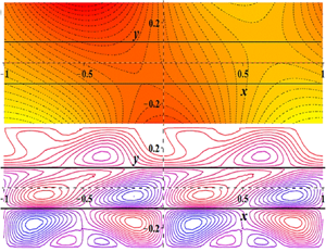
Figure 3. Thermal contours in the microchannel for different values of the phase difference between the wall thermal stimuli: (a)  $\theta = 0$, (b) $\theta = {\rm \pi}/2$ and (c) $\theta = {\rm \pi}$. Here, $T = (\bar{T} - \overline {{T_{min}}} )/(\overline {{T_{max}}} - \overline {{T_{min}}} )$. Parametric detail: $\overline {{T_l}} = 300\ \textrm{K},\overline {{T_u}} = 310\ \textrm{K},\alpha = 2{\rm \pi} ,$ $a:b:c = 1:1:1,{\lambda _a}:{\lambda _b}:{\lambda _c} = 1:1:1\ \textrm{and}\ {\delta _l} = {\delta _u} = 0.1$.

Figure 4. Interfacial temperatures for the ternary-liquid system for different values of the phase difference between the wall thermal stimuli at (a) the upper interface and (b) the lower interface. Here,  $T = (\bar{T} - \overline {{T_{min}}} )/(\overline {{T_{max}}} - \overline {{T_{min}}} )$. Parametric detail: $\overline {{T_l}} = 300\ \textrm{K},\overline {{T_u}} = 310\ \textrm{K},\alpha = 2{\rm \pi} ,$ $a:b:c = 1:1:1,{\lambda _a}:{\lambda _b}:{\lambda _c} = 1:1:1\ \textrm{and}\ {\delta _l} = {\delta _u} = 0.1$.

Figure 5. Streamfunction distribution in the microchannel, and its dependence on the phase difference and wall slip. Here,  $\psi = (\bar{\psi } - \overline {{\psi _{min}}} )/(\overline {{\psi _{max}}} - \overline {{\psi _{min}}} )$. Parametric detail: $\overline {{T_l}} = 300\ \textrm{K},\overline {{T_u}} = 310\ \textrm{K},\alpha = 2{\rm \pi} ,a:b:c $ $= 1:1:1,{\lambda _a}:{\lambda _b}:{\lambda _c} = 1:1:1,{\sigma _T} ={-} {10^{ - 4}}\ \textrm{N}\ \textrm{m}{\textrm{K}^{ - 1}},$ ${\mu _a}:{\mu _b}:{\mu _c} = 1:1:1,\mathrm{\epsilon } = {10^{ - 3}}\ \textrm{and}\ {\delta _l} = {\delta _u} = 0.1$.

Figure 6. Streamfunction distribution in the microchannel, and its dependence on the film thickness ratio of the three liquid layers and wall slip conditions. Here,  $\psi = (\bar{\psi } - \overline {{\psi _{min}}} )/(\overline {{\psi _{max}}} - \overline {{\psi _{min}}} )$. Parametric detail: $\overline {{T_l}} = 300\ \textrm{K},\overline {{T_u}} = 310\ \textrm{K},\alpha = 2{\rm \pi} ,$ $\theta = {\rm \pi}/2,{\lambda _a}:{\lambda _b}:{\lambda _c} = 1:1:1,{\sigma _T} ={-} {10^{ - 4}}\ \textrm{N}\ \textrm{m}{\textrm{K}^{ - 1}},$ ${\mu _a}:{\mu _b}:{\mu _c} = 1:1:1,\mathrm{\epsilon } = {10^{ - 3}}\ \textrm{and}\ {\delta _l} = {\delta _u} = 0.1$.
4.2. Thermal transport
To demonstrate the origin of the Marangoni convection, we first present the steady-state temperature distribution in the microchannel for the system configuration shown in figure 1. Figure 3 shows the distribution of the isotherms and its dependence on the phase difference between the two thermal stimuli applied at the top and the bottom wall  $(\theta )$. The plot is prepared by keeping the other influencing parameters fixed as: $\overline {{T_l}} = 300\ \textrm{K},\overline {{T_u}} = 310\ \textrm{K},\alpha = 2{\rm \pi} ,$ $a:b:c = 1:1:1,{\lambda _a}:{\lambda _b}:{\lambda _c} = 1:1:1\ \textrm{and}\ {\delta _l} = {\delta _u} = 0.1$. The local temperature is normalized using its extremums in the flow domain to make the charts more illuminating and understandable $(T = (\bar{T} - \overline {{T_{min}}} )/(\overline {{T_{max}}} - \overline {{T_{min}}} ))$. Due to the equal thermal conductivity and film thickness of the three fluid layers, the oscillation behaviours of the top and the bottom wall temperatures are replicated in the adjacent fluid layers, whereas the middle layer exhibits an intermediate pattern. Since the cause of the Marangoni convection is the interfacial temperature gradient, it is more important to understand the thermal behaviour of the interfaces. Therefore, we plot the variation of the temperatures at the two interfaces and explore their dependence on the phase difference between the two wall temperatures $(\theta )$ (refer to figure 4). The parametric combination chosen to prepare figure 4 is the same as that for figure 3. A lateral drift of the temperature profile is observed with changes in the thermal phase difference for the upper interface. However, the influence is marginal in the lower interface. The reason for this observation is the fact that the changes in the phase difference are incorporated by altering the top wall thermal stimulus, and due to equal thermal conductivity and film thickness of the fluid layers, the temperature of both the interfaces are decided by the walls closer to them.

Figure 7. Interfacial velocity profiles and their dependence on the film thickness ratio of the three liquid layers and wall slip conditions: (a) upper interface and (b) lower interface. Here,  $U = \bar{u}/\overline {{U_{max}}}$. Parametric detail: ${\mu _a}:{\mu _b}:{\mu _c} = 1:1:1,\mathrm{\epsilon } = {10^{ - 3}}\ \textrm{and}\ {\delta _l} = {\delta _u} = 0.1$ ${\mu _a}:{\mu _b}:{\mu _c} = 1:1:1,\mathrm{\epsilon } = {10^{ - 3}}\ \textrm{and}\ {\delta _l} = {\delta _u} = 0.1$.

Figure 8. Streamfunction distribution in the microchannel, and its dependence on the thermal conductivity ratio of the three liquid layers and wall slip conditions. Here,  $\psi = (\bar{\psi } - \overline {{\psi _{min}}} )/(\overline {{\psi _{max}}} - \overline {{\psi _{min}}} )$. Parametric detail: $\overline {{T_l}} = 300\ \textrm{K},\overline {{T_u}} = 310\ \textrm{K},\alpha = 2{\rm \pi} ,\theta = {\rm \pi} /2,a:b:c$ $= 1:1:1,{\sigma _T} ={-} {10^{ - 4}}\ \textrm{N}\ \textrm{m}{\textrm{K}^{ - 1}},{\mu _a}:{\mu _b}:{\mu _c}$ $= 1:1:1,\mathrm{\epsilon } = {10^{ - 3}}\ \textrm{and}\ {\delta _l} = {\delta _u} = 0.1$.
4.3. Hydrodynamic transport
We observe in the previous section that the periodic thermal stimuli provided at the walls incite periodic interfacial temperature profiles, which create variations in the interfacial tensions leading to the Marangoni or the TC effect. Further, the oscillatory nature of the gradients in the interfacial temperature or the interfacial tension prompt the circular (or vortical) motion of the fluid molecules, stimulating better mixing within the system. It is also observed that the patterned wettability at the walls can augment the flow pattern in a microchannel to enhance the mixing performance (Ghosh & Chakraborty Reference Ghosh and Chakraborty2012).
In our study, we explore the interplay of the patterned wall slip and thermal stimuli to obtain enhanced mixing in a microchannel. Figure 5 presents the streamfunction distribution for different thermal (or slip) phase differences  $(\theta )$ and compares the results for the no-slip and a finite slip $({l_s} = 0.1)$ condition at the microchannel walls (other parameters: ${\mu _a}:{\mu _b}:{\mu _c} = 1:1:1,\mathrm{\epsilon } = {10^{ - 3}}\ \textrm{and}\ {\delta _l} = {\delta _u} = 0.1$ ${\mu _a}:{\mu _b}:{\mu _c} = 1:1:1,\mathrm{\epsilon } = {10^{ - 3}}\ \textrm{and}\ {\delta _l} = {\delta _u} = 0.1$). It is observed that, while churning of the fluid molecules is restricted to the middle layer for the no-slip condition, it occurs in all three fluid layers when a finite slip is present at the walls. While the cause of the churning effect in the middle layer is attributed to the phase difference between the two interfacial temperatures, it is due to the interaction of the patterned wall slip and the periodic TC in the top and the bottom fluid layers. Further, the distortion of the vortices in the top and the bottom fluid layers due to patterned slip facilitates the mixing occurrence at larger length scales, which otherwise is confined to the local vortices. It is also noted that, although the changes in the thermal (or slip) phase difference $(\theta )$ have no serious effect on the mixing dynamics of the top and the bottom layer, they significantly alter the same in the middle layer. For the non-zero $\theta $, the vortex enveloping phenomenon is observed in the middle layer, resulting in better mixing, which is missing for $\theta = 0$. However, the mixing performance in the middle layer does not seem to be affected much by the wall slip conditions.

Figure 9. Interfacial velocity profiles and its dependence on the relative thermal conductivity of the three liquid layers and wall slip conditions: (a) upper interface and (b) lower interface. Here,  $U = \bar{u}/\overline {{U_{max}}} $. Parametric detail: $\overline {{T_l}} = 300\ \textrm{K},\overline {{T_u}} = 310\ \textrm{K},\alpha = 2{\rm \pi} ,\theta$ $= {\rm \pi}/2,a:b:c = 1:1:1,{\sigma _T} ={-} {10^{ - 4}}\ \textrm{N}\ \textrm{m}{\textrm{K}^{ - 1}},$ ${\mu _a}:{\mu _b}:{\mu _c} = 1:1:1,\mathrm{\epsilon } = {10^{ - 3}}\ \textrm{and}\ {\delta _l} = {\delta _u} = 0.1$.
We also plot the streamfunction distribution in the three liquid layers for different film thickness ratios (figure 6) to investigate the other possibilities of mixing intensification. The same parametric combination is used to prepare figure 6 as for figure 5, except that the phase difference is fixed to  $\theta = {\rm \pi}/2$ and the film thickness ratio is varied. It is observed that the fluid flows in the top layer of figure 6(b) and the bottom layer of figure 6(f) are highly chaotic and, hence, provide better mixing outcomes. The relatively large length scales enable better interplay of the wall slip and the interfacial TC effect in the cited cases. However, such a kind of vortex interaction is not observed in the absence of wall slip and, hence, the length scales at which mixing is occurring are restricted to the local diameters of the vortices (refer to figures 6a, 6c and 6e). To further understand the flow dynamics within the system, we plot the interfacial velocity profiles as a function of the film thickness ratio and the wall slip condition (refer to figure 7). The oscillation amplitude of the velocity seems to exhibit an inverse relation with its distance from the nearest wall. This is because the axial temperature gradient and, hence, the velocity at the interfaces due to TC is decided by the nearest wall thermal stimulus.

Figure 10. Streamfunction distribution in the microchannel, and its dependence on the phase difference  $(\theta )$ and wall slip conditions in a binary-liquid system. Here, $\psi = (\bar{\psi } - \overline {{\psi _{min}}} )/(\overline {{\psi _{max}}} - \overline {{\psi _{min}}} )$. Parametric detail: $\overline {{T_l}} = 300\ \textrm{K},\overline {{T_u}} = 310\ \textrm{K},\alpha = 2{\rm \pi} ,a:c$ $= 1:1,{\lambda _a}:{\lambda _c} = 1:1,{\sigma _T} ={-} {10^{ - 4}}\ \textrm{N}\ \textrm{m}{\textrm{K}^{ - 1}},$ ${\mu _a}:{\mu _c} = 1:1,\mathrm{\epsilon } = {10^{ - 3}}\ \textrm{and}\ {\delta _l} = {\delta _u} = 0.1$.

Figure 11. Streamfunction distribution in the microchannel, and its dependence on the film thickness ratio  $(a:c)$ and wall slip conditions in a binary-liquid system. Here, $\psi = (\bar{\psi } - \overline {{\psi _{min}}} )/(\overline {{\psi _{max}}} - \overline {{\psi _{min}}} )$. Parametric detail: $\overline {{T_l}} = 300\ \textrm{K},\overline {{T_u}} = 310\ \textrm{K},\alpha = 2{\rm \pi} ,\theta = {\rm \pi}/2,a:c = 1:1,{\sigma _T}$ $={-} {10^{ - 4}}\ \textrm{N}\ \textrm{m}{\textrm{K}^{ - 1}},{\mu _a}:{\mu _c} = 1:1,\mathrm{\epsilon } = {10^{ - 3}}\ \textrm{and}\ {\delta _l} = {\delta _u} = 0.1$.
Our study also explores the influence of the thermal conductivity ratio of the three fluid layers on the flow dynamics. A careful observation of figure 8 reveals that the flow strength is comparatively less in the liquid layer having lower thermal conductivity. This is due to the fact that the origin of the flow is based on the diffusion of the heat flux from the wall to the interfaces, which is directly proportional to the thermal conductivity of the medium. However, the disorder of the flow pattern suggests that better mixing is obtained in the fluid layer with a lower thermal conductivity as the mixing performance in the top and the bottom fluid layers is governed by the wall slip, and it dominates for a weak TC flow.

Figure 12. Streamfunction distribution in the microchannel, and its dependence on the relative thermal conductivity of the participating fluids  $({\lambda _a}:{\lambda _c})$ and wall slip conditions in a binary-liquid system. Here, $\psi = (\bar{\psi } - \overline {{\psi _{min}}} )/(\overline {{\psi _{max}}} - \overline {{\psi _{min}}} )$. Parametric detail: $\overline {{T_l}} = 300\ \textrm{K},\overline {{T_u}} = 310\ \textrm{K},\alpha = 2{\rm \pi} ,\theta = {\rm \pi}/2,{\lambda _a}:{\lambda _c} = 1:1,{\sigma _T}$ $={-} {10^{ - 4}}\ \textrm{N}\ \textrm{m}{\textrm{K}^{ - 1}},{\mu _a}:{\mu _c} = 1:1,\mathrm{\epsilon } = {10^{ - 3}}\ \textrm{and}\ {\delta _l} = {\delta _u} = 0.1$.
The variation of the interfacial velocity profiles as a function of the relative thermal conductivity of the fluid layers for slip and no-slip conditions at the walls is shown in figure 9. As expected, the magnitude of the interfacial velocity is large when the fluid layer, which is positioned between the interface and the wall, has higher thermal conductivity. It is also noted that no significant influence of the wall slip is observed in both the interfacial velocities. This explains the earlier observation that the mixing performance of the middle layer does not seem to alter much by changing the wall slip conditions (see figures 5, 6, and 7). Further, a comparative observation of figures 6 and 8, and figures 7 and 9 reveals that the impacts of the fluids’ thermal conductivity and film thickness ratios are reversed but equally authoritative, as follows from Fourier's law of heat conduction  $(q^{\prime\prime} = \lambda (\partial T/\partial n))$.

Figure 13. Interfacial deformation and its dependence on the relative film thickness of the three liquid layers and wall slip conditions: (a) upper interface and (b) lower interface. Here,  ${y_i} = {\bar{y}_i}/\overline {{l_c}}$, where $i = l,u$. Parametric detail: $\overline {{T_l}} = 300\ \textrm{K},\overline {{T_u}} = 310\ \textrm{K},\alpha = 2{\rm \pi} ,\theta = {\rm \pi}/2,{\lambda _a}:{\lambda _b}:{\lambda _c}$ $= 1:1:1,{\sigma _T} ={-} {10^{ - 4}}\ \textrm{N}\ \textrm{m}{\textrm{K}^{ - 1}},{\mu _a}:{\mu _b}:{\mu _c}$ $= 1:1:1,\mathrm{\epsilon } = {10^{ - 3}}\ \textrm{and}\ {\delta _l} = {\delta _u} = 0.1$.
We continue the discussion by focusing on a binary-liquid system that is created when the middle layer thickness tends to zero  $(b \to 0)$ in a simplified model of the current issue. Figure 10 shows the streamfunction distribution and how it depends on the phase difference $(\delta )$ and wall slip conditions in a binary-liquid system. It is observed from figure 10 that the relative shift of the streamline contours in different liquid layers, which appeared in ternary-liquid system for non-zero $\theta $ value (see figure 5), is missing in the binary-liquid system. This observation can be understood by noting that the flow is generated at the interfaces due to gradients in interfacial temperatures. Two interfaces exist for a ternary-liquid system whose temperature fluctuations are decided mainly by the nearest wall. Hence, the temperature of the two interfaces will have phase differences for non-zero $\theta $, leading to distortion of vortices in the middle layer and a visible shift in streamline contours in the top and the bottom liquid layer. However, whenever a phase difference exists between the two wall temperatures, the presence of a single interface in the binary-liquid system shifts streamline contours in both liquid layers by an equal amount. Hence, the relative displacement between the streamline contours in the top and bottom layers is zero. However, there is a net displacement of streamline contours in both of the liquid layers with respect to the $y = 0$ line. Further, in the absence of wall slip, the system's mixing performance does not appear to be dependent on $\delta $.

Figure 14. Comparison of the steady-state species distribution in a fully developed laminar flow and the Marangoni flow. Here,  $C = (\bar{C} - \overline {{C_{min}}} )/(\overline {{C_{max}}} - \overline {{C_{min}}} )$. Other parametric detail: $\overline {{T_l}} = 300\ \textrm{K},\overline {{T_u}} = 310\ \textrm{K},\alpha = 2{\rm \pi} ,\theta = {\rm \pi}/2,a:b:c = 1:1:1,{\lambda _a}:{\lambda _b}:{\lambda _c}$ $= 1:1:1,{\sigma _T} ={-} {10^{ - 4}}\ \textrm{N}\ \textrm{m}{\textrm{K}^{ - 1}},{\mu _a}:{\mu _b}:{\mu _c} = 1:1:1,{l_s}$ $= 0.1,\mathrm{\epsilon } = {10^{ - 3}}\ \textrm{and}\ {\delta _l} = {\delta _u} = 0.1$.
A close observation of figures 10(b) and 10(f) reveals that the presence of a phase difference  $(\theta )$ in the boundary conditions leads to net transport of the fluids in the axial direction. The influence of the relative film thickness and the relative thermal conductivity of the participating fluids is also demonstrated in figures 11 and 12, respectively. It is clear that the vortex distortion is only discernible for slip boundary conditions at the walls. Consequently, the interaction between the system's thermal stimuli and wall wettability can be comfortably attributed for this result. Better mixing is attained in a fluid layer with a larger thickness, similar to the ternary-liquid system for a configuration with varied fluid layer film thicknesses.

Figure 15. Species concentration distribution in the middle liquid layer across the microchannel length at different axial locations. Here,  $\bar{x}$ is in μm, ${y^\ast } = \bar{y}/\bar{b}$ and $C = (\bar{C} - \overline {{C_{min}}} )/(\overline {{C_{max}}} - \overline {{C_{min}}} )$. Other parametric detail: $\overline {{T_l}} = 300\ \textrm{K},\overline {{T_u}} = 310\ \textrm{K},\alpha = 2{\rm \pi} ,\theta = {\rm \pi}/2,a:b:c = 1:1:1,{\lambda _a}:{\lambda _b}:{\lambda _c} $ $= 1:1:1,{\sigma _T} ={-} {10^{ - 4}}\ \textrm{N}\ \textrm{m}{\textrm{K}^{ - 1}},{\mu _a}:{\mu _b}:{\mu _c}$ $= 1:1:1,{l_s} = 0.1,\mathrm{\epsilon } = {10^{ - 3}}\ \textrm{and}\ {\delta _l} = {\delta _u} = 0.1$.

Figure 16. Validation of the mathematical formulations with the numerical simulations: (a) thermal result, (b) hydrodynamic result. Parametric detail:  $\overline {{T_l}} = \overline {{T_u}} = 300\ \textrm{K},{\delta _l} = {\delta _u} = 0.1,\alpha = 2{\rm \pi} ,\theta = 0,x = 0.3$.
It is also observed that the flow dynamics is not significantly influenced by the thermal conductivity ratio of the fluid layers, as may be inferred from figure 12. Earlier, it was found that the flow strength for the fluid layer with significantly lower thermal conductivity was low for a ternary-liquid system (see figure 8). This observation was attributed to insufficient heat conduction from the wall to the closest interface. However, since there is only one interface in a binary-liquid system, heat diffusion through the fluid layer with the higher thermal conductivity determines the variation in interfacial temperature.
4.4. Interface deformation behaviour
In this section, we explain the credibility of the flat and undeformed interface assumption. Figure 13 presents the profiles of the deformed interfaces obtained by using the previous solutions on the streamfunction distribution (other parameters:  $= 1:1:1,{\sigma _T} ={-} {10^{ - 4}}\ \textrm{N}\ \textrm{m}{\textrm{K}^{ - 1}},{\mu _a}:{\mu _b}:{\mu _c}$ $= 1:1:1,\mathrm{\epsilon } = {10^{ - 3}}\ \textrm{and}\ {\delta _l} = {\delta _u} = 0.1$ $= 1:1:1,{\sigma _T} ={-} {10^{ - 4}}\ \textrm{N}\ \textrm{m}{\textrm{K}^{ - 1}},{\mu _a}:{\mu _b}:{\mu _c}$ $= 1:1:1,\mathrm{\epsilon } = {10^{ - 3}}\ \textrm{and}\ {\delta _l} = {\delta _u} = 0.1$). The effect of the film thickness ratio and the wall slip boundary conditions on the interfacial deformation is also demonstrated. The most critical observation drawn from figure 13 is the order of the deformation relative to the system length scale $({y_i} = {\bar{y}_i}/\overline {{l_c}} \sim {10^{ - 3}})$. The small deformation of the interfaces, despite the presence of circular motion of the participating fluids, is attributed to the low capillary number $(Ca\sim {10^{ - 6}})$ in the present study. The deformation of the interface is small enough to be neglected relative to the system length scale. It is also observed that the wall slip's influence on the interfaces’ deformed profile is imperceptible. However, the deformed interfaces’ profiles seem to depend on the film thickness ratio. The extent of deformation is inversely related to its distance from the closest wall.

Figure 17. Velocity contours in the ternary-liquid system for the discrete wall temperature conditions, obtained from numerical solutions. The colour bar shown is in logarithmic scale. Parametric detail: bottom and top layers are kerosene oil, middle layer is water,  $\overline {{T_l}} = 300\ \textrm{K},\overline {{T_u}} = \left\{{\begin{array}{@{}c} {340\ \textrm{K}\ \textrm{for}\ N + 0.75 < x < N + 1.25}\\ {315 \ \textrm{K}\ \textrm{for}\ N + 0.25 < x < N + 0.75} \end{array}} \right.\!\!\!\!.$
4.5. Solute transport
To consolidate the point that an enhanced mixing is obtained by the interplay of the TC effect and the patterned wettability, we compare the steady-state species distribution in a microchannel due to a fully developed laminar flow and the thermal Marangoni flow (refer to figure 14). The other involved parameters are kept fixed to perform the analysis  $(\overline {{T_l}} = 300\ \textrm{K},\overline {{T_u}} = 310\ \textrm{K},\alpha = 2{\rm \pi} ,\theta = {\rm \pi}/2,a:b:c = 1:1:1,{\lambda _a}:{\lambda _b}:{\lambda _c}$ $= 1:1:1,{\sigma _T} ={-} {10^{ - 4}}\ \textrm{N}\ \textrm{m}{\textrm{K}^{ - 1}},{\mu _a}:{\mu _b}:{\mu _c}$ $= 1:1:1,\mathrm{\epsilon } = {10^{ - 3}}\ \textrm{and}\ {\delta _l} = {\delta _u} = 0.1)$. The order of the Péclet number $(Pe)$ for the solute transport analysis is ${\sim} O(1)$. To make the comparison more realistic, we take the thicknesses of the three fluid layers in our study and that of the film undergoing fully developed laminar flow to be the same (4 μm). A discrete inlet concentration profile (table 6) is provided in both cases, and how fast the uniformity in the species concentration across the cross-section is attained is explored. We found that the mixing length (length scale required to attain full mixing) for the fully developed flow is 10 times larger than that for the thermal Marangoni flow. The transverse diffusion or dispersion determines the species transport across the microchannel axis in a fully developed flow as the flow is unidirectional, and there is no convection current in this direction. However, the circular motion due to the periodic thermal stimuli enables the species convection in both the lateral and the transverse direction in the Marangoni convection.

Figure 18. Interfacial temperatures of the ternary-liquid system for the discrete wall temperature conditions: (a) the upper interface and (b) the lower interface. Here,  $T = (\bar{T} - \overline {{T_{min}}} )/(\overline {{T_{max}}} - \overline {{T_{min}}} )$. Parametric detail: bottom and top layers are kerosene oil, middle layer is water, $\overline {{T_l}} = 300\ \textrm{K}, \overline {{T_u}} = \left\{ {\begin{array}{@{}c} {340\ \textrm{K}\ \textrm{for}\ N + 0.75 < x < N + 1.25}\\ {315\ \textrm{K}\ \textrm{for}\ N + 0.25 < x < N + 0.75} \end{array}} \right.\!\!\!\!.$
To extend the discussion further, we also plot the cross-sectional variation of the species concentration profiles for the TC flow at different the axial locations (see figure 15). The other parametric detail is kept the same as that for figure 14. The study is presented only for the middle fluid layer as similar behaviour is shown by the other two liquid layers as well (which is also clear from figure 14). The uniformity of the solute concentration is obtained within  $2\ \mathrm{\mu }\textrm{m}$ of axial transport from the inlet, which manifests the rapid mixing ability of the present configuration.

Figure 19. Interfacial velocities of the ternary-liquid system for the discrete wall temperature conditions: (a) the upper interface and (b) the lower interface. Here,  $U = \bar{u}/\overline {{U_{max}}} $. Parametric detail: bottom and top layers are kerosene oil, middle layer is water, $\overline {{T_l}} = 300\ \textrm{K},\overline {{T_u}} = \left\{ {\begin{array}{@{}c} {340\ \textrm{K}\ \textrm{for}\ N + 0.75 < x < N + 1.25}\\ {315\ \textrm{K}\ \textrm{for}\ N + 0.25 < x < N + 0.75} \end{array}} \right.\!\!\!\!.$
It is to be noted here that the quantitative comparisons of the mixing performance for the different parametric combinations is not provided in the present work as the study is restricted to steady-state analysis. Since there is no net flow in the present configuration due to periodic boundary conditions, the steady-state species distribution within each fluid layer becomes independent of the wall slip condition. However, it is predicted from the streamfunction distributions (shown in figures 5, 6, 8, 10, 11 and 12) that the time scale to reach the steady condition would be much shorter if the patterned slip condition is imposed at the microchannel walls. The quantitative justification for the arguments can be provided by performing transient analysis of the problem, which is beyond the scope of the present paper.
5. Numerical simulations
We also validate the analytical solutions for the thermal and hydrodynamic transport with the finite-element-based numerical simulations performed in COMSOL Multiphysics. The thickness and periodic length (length of the computational domain) of the three liquid layers are  $20\ \mathrm{\mu }\textrm{m}$ and $100\ \mathrm{\mu }\textrm{m}$, respectively. The origin of the coordinate system is located at the centre of the middle layer. The flow domain is discretized using the structured mesh formation with the maximum grid size of $0.5\ \mathrm{\mu }\textrm{m}$. The patterned wall thermal stimuli, as shown in figure 1 with no-slip conditions, are applied at the confining walls (with $\overline {{T_l}} = \overline {{T_u}} = 300\ \textrm{K},{\delta _l} = {\delta _u} = 0.1,\alpha = 2{\rm \pi} ,\theta = 0$), and the properties of the liquid layers are taken to be same as those in the analytical solution. Further, periodic conditions are used at the lateral boundaries of the computational domain. The Marangoni effect couples the heat transfer and laminar flow module in the simulations, and the phase field method is employed to track the interfaces. The temperature and velocity variations across the interfaces at an axial location of $30\ \mathrm{\mu }\textrm{m}$ or $x = 0.3$ (normalized dimension) are compared for the analytical and the numerical solutions in figure 16. The temperature and the velocity are normalized with their corresponding maximum values to make the comparison.
We extend the numerical simulations performed to a discrete wall temperature condition applied to the kerosene oil–water–kerosene oil system, so that the simulation results can be experimentally replicated in the future. The top wall temperature is taken to be of the square wave form (5.1) and the bottom wall temperature is kept constant at  $300\ \textrm{K}$. The contour plot for the velocity field along with the streamlines is shown in figure 17 and the interfacial temperature and velocity profiles in figures 18 and 19, respectively,
 \begin{equation}\overline {{T_u}} =
\left\{ {\begin{array}{@{}l@{}} {340\ \textrm{K}\quad
\textrm{for}\ N + 0.75 < x < N + 1.25}\\ {315\
\textrm{K}\quad \textrm{for}\ N + 0.25 < x < N + 0.75}
\end{array},\quad \textrm{where}\ N\ \textrm{is}\
\textrm{an}\ \textrm{integer}\textrm{.}}
\right.\end{equation}
\begin{equation}\overline {{T_u}} =
\left\{ {\begin{array}{@{}l@{}} {340\ \textrm{K}\quad
\textrm{for}\ N + 0.75 < x < N + 1.25}\\ {315\
\textrm{K}\quad \textrm{for}\ N + 0.25 < x < N + 0.75}
\end{array},\quad \textrm{where}\ N\ \textrm{is}\
\textrm{an}\ \textrm{integer}\textrm{.}}
\right.\end{equation}
Further, we obtain the steady-state species distribution in the fluid layers for a Dirichlet inlet concentration condition as taken for the analytical solution (table 6). The species transport equation is solved via the ‘transport of dilute species’ module of the COMSOL Multiphysics. We present the contour plot of the steady-state concentration distribution and the transverse variation of the local species concentration at different axial positions for the middle layer in figure 20. Similar distributions were observed for the top and bottom layers, and, hence, the results are presented only for the middle layer to avoid repetition. The coordinate axes are normalized using the thickness of the middle layer to make the figures more informative  $({x^\ast } = \bar{x}/\bar{b},{y^\ast } = \bar{y}/\bar{b})$. The transverse variation of the species concentration becomes negligible after ${x^\ast } = 0.5$, demonstrating the good mixing performance of the system due to the vortical motions.

Figure 20. Species concentration distribution in the middle liquid layer: (a) contour plot of C, (b) transverse variation of C at different axial locations. Here,  ${x^\ast } = \bar{x}/\bar{b}$, ${y^\ast } = \bar{y}/\bar{b}$ and $C = (\bar{C} - \overline {{C_{min}}} )/(\overline {{C_{max}}} - \overline {{C_{min}}} )$. Parametric detail: bottom and top layers are kerosene oil, middle layer is water, $\overline {{T_l}} = 300\ \textrm{K}, \overline {{T_u}} = \left\{ {\begin{array}{@{}c@{}} {340\ \textrm{K}\ \textrm{for}\ N + 0.75 < x < N + 1.25}\\ {315\ \textrm{K}\ \textrm{for}\ N + 0.25 < x < N + 0.75} \end{array}} \right.$.
6. Conclusions
In this study, we explore the interplay of the periodic thermal stimuli and patterned wettability at the microchannel walls to enhance the mixing performance of the ternary-liquid system. We consider first- and second-harmonic periodic profiles for the wall slip and temperature boundary conditions. The inclusion of the second harmonic in the thermal boundary condition is a mathematical requirement of the problem to incorporate the periodic behaviour of the wall slip in the subsequent analysis. An asymptotic approach is applied to obtain a semi-analytical solution to the decoupled energy and Navier–Stokes equation by the perturbation technique. We determine the controlling non-dimensional numbers  $(Re \sim {10^{ - 3}},Ma \sim {10^{ - 3}}\ \textrm{and}\ Ca \sim {10^{ - 6}})$ by using an order of magnitude analysis, to explain the applicability of the decoupled governing equations. Our study is based on the crucial premise that the interfaces remain nearly undeformed, which is later confirmed by obtaining approximate profiles of the interfaces. The deformation undergone by the interfaces is ${y_i} = {\bar{y}_i}/\overline {{l_c}} \sim {10^{ - 3}}$, which is negligible compared with the system length scale. We have also performed numerical simulations for the thermal and hydrodynamic transport of a ternary-liquid system and compared the results with the analytical solutions. Further, the numerical simulation is extended to discrete wall temperatures (square wave form) and the corresponding flow characteristics are presented.
The circular motion generated by the oscillating nature of the driving stimuli provides excellent blending in all three fluid layers. The mixing effectiveness of the suggested arrangement is consolidated by comparing the species transport in the present study and the fully developed laminar flow. To obtain the steady-state species distribution in the microchannel for a discrete inlet concentration, the species transport equation is numerically solved in COMSOL Multiphysics for both the present flow pattern and the fully developed flow. The mixing length in the present model is found to be 10 times shorter than that in the fully developed flow, indicating better mixing performance. The enhanced mixing obtained in our work is ascribed to the convective transport of the solute particles across the microchannel axis by the circular vortices, which are missing in a fully developed laminar flow.
In order to achieve the best configuration for the current system, we further investigate the impact of various parameters. The wettability pattern of the walls has a significant impact on the mixing performance in the fluid layers that are in direct contact with them. The patterned wall slip interacts with the TC formed at the interfaces to distort the flow vortices in the top and bottom fluid layers, enhancing the churning effect. The thermal conductivity and film thickness of the fluid layers also seemed to have significant impacts on the mixing dynamics of the top and bottom fluid layers. However, we find that the aforementioned characteristics have no appreciable influence on the middle layer's ability to mix, which can instead be modulated by altering the phase difference between the thermal (or slip) stimuli at the two walls. Lastly, we illustrate the flow dynamics in a binary-liquid system using a simplified model with zero middle layer  $(b \to 0)$.
Funding
The authors thank IIT Kharagpur for supporting the work through internal funds.
Declaration of interests
The authors report no conflict of interest.
Appendix
Table 7. The boundary conditions to obtain solutions for  $g_j^i(\kern0.7pt y)$.

Table 8. The boundary conditions to obtain solutions for  $h_j^i(\kern0.7pt y)$.


