


1. Introduction
Yield-stress fluid flows through porous media are inherent to many industries including filtration, oil and gas, mining (Frigaard, Paso & de Souza Mendes Reference Frigaard, Paso and de Souza Mendes2017) and also numerous other applications such as biomedical treatments (Keating, Hajducka & Harper Reference Keating, Hajducka and Harper2003). Although in the case of Newtonian fluids many aspects of flows in porous media are well-discussed in the literature, when it comes to yield-stress fluids, our understanding of the phenomenon is limited mainly because modelling this problem is cumbersome due to the computational costs and/or the complexity of the experiments needed to carry out the analysis.
To overcome these barriers, several studies focused on pore-scale features of this problem (Bleyer & Coussot Reference Bleyer and Coussot2014; Shahsavari & McKinley Reference Shahsavari and McKinley2016; De Vita et al. Reference De Vita, Rosti, Izbassarov, Duffo, Tammisola, Hormozi and Brandt2018; Bauer et al. Reference Bauer, Talon, Peysson, Ly, Batôt, Chevalier and Fleury2019; Waisbord et al. Reference Waisbord, Stoop, Walkama, Dunkel and Guasto2019; Chaparian et al. Reference Chaparian, Izbassarov, De Vita, Brandt and Tammisola2020), however, it is yet unclear how to link/upscale the studies in microscale to macroscale, especially due to the nonlinearity of the constitutive equations which renders the bulk transport properties unpredictable from pore-scale dynamics. Nevertheless, in the intricate transport mechanism of yield-stress fluids through porous media, several mutual features can be identified regardless of the scales on which the previous studies are focused. In a number of studies (Talon & Bauer Reference Talon and Bauer2013; Liu et al. Reference Liu, De Luca, Rosso and Talon2019; Chaparian & Tammisola Reference Chaparian and Tammisola2021; Talon Reference Talon2022), four regimes are detected in terms of flow rate ( $Q$)-applied pressure gradient ( $\Delta P/L$): (i) when the applied pressure gradient is less than a critical pressure gradient ( $\Delta P_c/L$), there is no flow ( $Q=0$); (ii) if the applied pressure gradient slightly exceeds the critical value, the flow is extremely localised in a channel and the flow rate linearly scales with the excessive pressure gradient where other parts of the fluid are quiescent; (iii) the third regime emerges when the applied pressure gradient increases, more and more channels appear (moderate values of pressure gradient) and the flow rate scales quadratically with the excessive applied pressure gradient; (iv) finally, when the applied pressure gradient is much higher than the critical value, the flow rate again scales linearly with the excessive pressure gradient.
Although these generic features/scales have been evidenced in a large number of studies, still the lack of an inclusive Darcy type expression for bulk properties is evident. The very first step for finding such a generic model is to thoroughly understand the pressure gradient threshold and more generally the yield limit which scaffolds any further progression of this aim.
In spite of the previous efforts to address the yield limit of the current problem (Liu et al. Reference Liu, De Luca, Rosso and Talon2019; Chaparian et al. Reference Chaparian, Izbassarov, De Vita, Brandt and Tammisola2020; Fraggedakis, Chaparian & Tammisola Reference Fraggedakis, Chaparian and Tammisola2021), mostly the findings are case dependent, thereby limiting their application for more complicated practical systems. As discussed, in this limit the flow is extremely heterogeneous, hence, pore-scale studies are not fully reliable since they do not contain any statistical data in ‘real’ porous media where a wider range of length scales are involved. Thus, in the present study, the aim is to derive a theoretical model based on yield-stress fluid flows principles and then validate the proposed model with exhaustive simulations.
To this end, we construct our porous media by randomly distributed obstacles of various shapes and lengths to avoid any biased results. Namely, three major types of obstacles are considered: circles, squares and polygons. Then, fluid flow simulations based on the adaptive augmented Lagrangian approach (Roquet & Saramito Reference Roquet and Saramito2003; Glowinski & Wachs Reference Glowinski and Wachs2011) are performed which is shown to be a reliable tool for investigating the present problem, especially at the yield limit where non-regularised rheology is essential (Frigaard & Nouar Reference Frigaard and Nouar2005). To be fit for purpose, both monodispersed and bidispersed systems are considered. We have recently delved into the study of monodispersed circular obstacles by means of pore-network approaches where a large data set has been generated (Fraggedakis et al. Reference Fraggedakis, Chaparian and Tammisola2021). This data set is adopted here in conjunction with the present computational data for further validation of the proposed theory.
The outline of the present paper is as follows. The problem is described in § 2.1 and the details of the utilised numerical method and porous media construction are highlighted. The numerical results are given in § 3. The theory is developed in § 4 and the comparison with the computational results is performed. Conclusions are drawn in § 5.
2. Problem description
2.1. Mathematical formulation
We consider incompressible two-dimensional Stokes flow through a set of obstacles (i.e.  $X$) in a box of size $L \times L$ (i.e. $\varOmega$) which is governed by
 \begin{equation} 0 =-\boldsymbol{\nabla} p + \boldsymbol{\nabla} \boldsymbol{\cdot} \boldsymbol{\tau}\quad{\rm and}\quad\boldsymbol{\nabla} \boldsymbol{\cdot} \boldsymbol{u}=0\quad \text{in}\ \varOmega \setminus \bar{X}, \end{equation}
where  $p$,
$p$,  $\boldsymbol {\tau }$ and $\boldsymbol {u}$ represent the pressure, deviatoric stress tensor and the velocity vector of the fluid, respectively. We use the Bingham model to describe the fluid's rheology,
 \begin{equation} \left\{\begin{array}{@{}ll} \boldsymbol{\tau} = \left( 1 + \displaystyle{\dfrac{B}{\Vert \dot{\boldsymbol{\gamma}} \Vert}} \right) \dot{\boldsymbol{\gamma}} & \mbox{iff}\ \Vert \boldsymbol{\tau} \Vert > B, \\[10pt] \dot{\boldsymbol{\gamma}} = \boldsymbol{0} & \mbox{iff}\ \Vert \boldsymbol{\tau} \Vert \leq B, \end{array} \right. \end{equation}
in which  $\dot {\boldsymbol {\gamma }}$ is the rate of strain tensor (i.e. $\boldsymbol {\nabla } \boldsymbol {u} + \boldsymbol {\nabla } \boldsymbol {u}^T$) and $\Vert {\cdot } \Vert$ is the second invariant of the tensor. Therefore, yielding obeys the von Mises criterion.
The above equations are non-dimensional and  $B=\hat {\tau }_y \hat {\ell } / \hat {\mu } \hat {V}$ is the Bingham number, where $\hat {\mu }$ is the plastic viscosity of the Bingham fluid, $\hat {V}$ is the mean inlet velocity and $\hat {\ell }$ is the characteristic length scale which will be fixed later in § 2.2. Hence, the Bingham number is the ratio of the yield stress of the fluid to the characteristic viscous stress. To derive equations (2.1) and (2.2), we use the following scalings:
 \begin{equation} \left( x,y \right) = \frac{\left( \hat{x},\hat{y} \right)}{\hat{\ell}},\quad\boldsymbol{u}=\left( u,v \right) = \frac{(\hat{u},\hat{v})}{\hat{V}}\quad {\rm and}\quad \left(\kern 1.5pt p,\boldsymbol{\tau} \right)=\frac{\left(\hat{p},\hat{\boldsymbol{\tau}}\right)}{\hat{\mu} \hat{V}/\hat{\ell}}, \end{equation}
where  $x$ and $y$ are the coordinates in the streamwise and spanwise directions, respectively (see figure 1). Please note that all the variables with a hat ( $\hat {\cdot }$) are dimensional throughout the paper; the same symbols are used for the dimensionless parameters without a hat.

Figure 1. Schematic of the coordinate system directions and the inlet length  $L_{inl}$ which in this case consists of two segments depicted in blue.
As mentioned above,  $\hat {V}$ is the mean inlet velocity, hence
 \begin{equation} \hat{V} = \frac{\displaystyle\int\hat{u}\,\text{d}\hat{y}}{\hat{L}_{inl}} \Rightarrow 1 = \frac{\displaystyle\int (\hat{u}/\hat{V}) \,\text{d}y }{(\hat{L}_{inl}/\hat{\ell})} \Rightarrow Q = \int u \,\text{d}y = L_{inl}, \end{equation}
where  $Q$ is the flow rate and $L_{inl}$ is the length of the domain's inlet, i.e. the obstructed length by the solid obstacles is subtracted from $L$ to calculate $L_{inl}$ (see figure 1). Therefore, in this setting, the flow rate is always equal to $L_{inl}$, irrespective of the Bingham number. This approach in formulating the present problem is called resistance formulation or [R]. Indeed, the yield limit in this type of problem set-up moves to $B \to \infty$. We will predominantly use this approach in our following simulations and analytical derivations. Alternatively, another formulation is possible: mobility formulation or [M].
In the [M] approach, the applied pressure gradient is used to scale the pressure and the stress tensor (i.e.  $({\Delta \hat {P}}/{\hat {L}})\hat {\ell }$), while the velocity vector is scaled with $({\hat {\ell }^2}/{\hat {\mu }})({\Delta \hat {P}}/{\hat {L}})$. Hence, as a result, the non-dimensional applied pressure gradient in [M] is always equal to unity.
In the [M] formulation, the independent flow parameter is
 \begin{equation} Y = \frac{\hat{\tau}_y }{\hat{\ell} (\Delta \hat{P}/\hat{L})}, \end{equation}
which is known as the yield number. Indeed, the flow rate changes as the yield number varies: it is zero when  $Y \geq Y_c$ and increases as the yield number drops below $Y_c$ and decreases. Indeed, the yield limit in [M] is marked by $Y_c$ which is the critical yield number; if $Y < Y_c$, the applied pressure gradient is enough to overcome the yield stress resistance and the fluid flows inside the medium.
There is a one-to-one map between the [R] and [M] approaches: these two distinct formulations are linked together by  $Y (\Delta P/L) = B$. This makes the interpretation of the results feasible; no matter whether the analysis (analytical, computational, etc.) is done in the [R] or [M] settings. For more detailed explanations of these two formulations in porous media flows or more general pressure-driven flows, readers are referred to Chaparian & Tammisola (Reference Chaparian and Tammisola2021).
2.2. Porous media construction
To construct the porous media for the fluid flow simulations, we randomly distribute non-overlapping obstacles ( $X$) inside a square domain ( $\varOmega$) of size $L \times L = 50 \times 50$, see figure 2. Indeed, the centre of each obstacle is chosen randomly with uniform distribution in the interval $[ -\epsilon, L + \epsilon ] \times [ -\epsilon, L + \epsilon ]$ and then it will be checked if the obstacle satisfies the non-overlapping condition. Here $\epsilon$ is introduced to let the obstacles cross the computational borders.

Figure 2. Schematic of the porous media where (a–c) are monodispersed topologies and (d–f) are bidispersed ones: (a,d) square obstacles; (b,e) circular obstacles; (c,f) generated polygon obstacles based on Voronoi tessellation of panels (b,e).
Three different obstacle topologies are used: circles, squares and polygons. We consider monodispersed and bidispersed cases. In the monodispersed circular cases, the radius of the obstacles is used as the length scale,  $\hat {\ell }=\hat {R}$, from which we deduce that each individual obstacle area is equal to ${\rm \pi}$. In the monodispersed square cases, to be consistent, the individual area of an obstacle is again ${\rm \pi}$ or indeed $\hat {\ell } = \sqrt {\hat {L}_s/{\rm \pi} }$ where $\hat {L}_s$ is the length of squares’ edges.
In the bidispersed cases, the area of the larger obstacles is  $25{\rm \pi}$ while the area of the smaller ones is still ${\rm \pi}$. This is the only parameter which is fixed in the construction of bidispersed cases. To ensure generality of the results, both the positions and the number of the larger obstacles are also chosen completely randomly.
For the case of polygons (see figure 2c,f), firstly the domain is partitioned based on the Voronoi tessellation in which the centres of circles are adopted as the set of points in the Euclidean plane. Then each Voronoi cell (the edges of cells are depicted in red in figure 2) is squeezed (or expanded in the bidispersed cases) to get the desired area of  ${\rm \pi}$ (or $25 {\rm \pi}$ in the bidispersed cases). Hence, this method provides us with a variety of shapes for the polygon cases.
As mentioned, here we are interested in two-dimensional flows, hence, the solid ‘volume’ fraction in the porous media is denoted by  $\phi =\text {meas}(X)/\text {meas}(\varOmega )$. Therefore, the porosity of the medium (i.e. void fraction) can be represented simply by $1-\phi$.
Note that in the polygon bidispersed cases, the obstacles may weakly overlap because of the expansion of the cells associated with the larger obstacles. In these cases, the effective solid volume fraction is considered.
2.3. Computational details
We implement an augmented Lagrangian method to simulate the viscoplastic fluid flow (Roquet & Saramito Reference Roquet and Saramito2003; Glowinski & Wachs Reference Glowinski and Wachs2011). This method is capable of handling the non-differentiable Bingham model by relaxing the rate of the strain tensor. An open-source finite element environment – FreeFEM $++$ (Hecht Reference Hecht2012) – is used for discretisation and meshing, which has been widely discussed and validated in our previous studies, for more details (choice of elements, etc.) please see Chaparian & Frigaard (Reference Chaparian and Frigaard2017), Iglesias et al. (Reference Iglesias, Mercier, Chaparian and Frigaard2020), Chaparian & Tammisola (Reference Chaparian and Tammisola2021) and Chaparian, Owens & McKinley (Reference Chaparian, Owens and McKinley2022). The anisotropic adaptive mesh in $\varOmega /\bar {X}$ is combined with this method to get high resolution of the flow features and more accurate results. Details about the mesh adaptation can be found in Roquet & Saramito (Reference Roquet and Saramito2003) and Chaparian & Tammisola (Reference Chaparian and Tammisola2019). Basically, the initial mesh is adapted on the piecewise linear approximation of the Hessian of the square root of the dissipation function which results in a finer mesh in sheared regions and a coarser mesh in unyielded regions. Also the adapted mesh is stretched anisotropically to align with the yield surfaces (boundary between unyielded and yielded regions), see figure 3.

Figure 3. Mesh generation for a sample case: (a) initial mesh (‘uniform’ coarse grid); (b) final mesh after six cycles of adaptation. This mesh is associated with the simulation illustrated in panel (d) of figure 4. Note that only part of the mesh in the white window of panel (d) of figure 4 (at the pore-scale) is shown here.
Regarding the velocity boundary conditions: (i) no-slip is imposed at the surface of the obstacles (i.e.  $u=v=0$); (ii) a natural boundary condition (or ‘non-essential’ finite element boundary condition) is imposed on the inlet (left face) and the outlet (right face), $\partial u/\partial x =0$; and (iii) free-slip on the top and bottom edges, $\partial u/\partial y =0$.
As discussed in § 2.1, in [R] setting, the flow rate must be equal to  $L_{inl}$, hence, the imposed pressure gradient $\Delta P/L$ (which is a body force term in the numerical implementation) will be iterated to match the flow rate (Roustaei, Gosselin & Frigaard Reference Roustaei, Gosselin and Frigaard2015).
In the present study, a number of simulations are performed at different porosities to validate the scaling which will be derived in § 4. As mentioned in § 1, the main aim here is presenting a mathematical model for the yield limit based on physical features of the problem, and then validating it with the present simulations and the previous published data. Due to the high computational cost of the full fluid flow simulations, we do not follow a statistical approach by simulating the flow in many realisations here. Rather, we use our data previously published in Fraggedakis et al. (Reference Fraggedakis, Chaparian and Tammisola2021) which will be discussed later in § 4. Recent advances in computational methods of viscoplastic fluids (e.g. known as PAL (penalized augmented Lagrangian) and FISTA (fast iterative shrinkage/thresholding algorithm) methods) accelerate the simulations of this type of fluids, yet the implementation of these methods is beyond the scope of this work. Interested readers are referred to Dimakopoulos et al. (Reference Dimakopoulos, Makrigiorgos, Georgiou and Tsamopoulos2018), Treskatis, Moyers-González & Price (Reference Treskatis, Moyers-González and Price2016) and Treskatis et al. (Reference Treskatis, Roustaei, Frigaard and Wachs2018).
3. Illustrated examples
Figure 4 shows the flow in the six sample geometries at  $\phi =0.45$ and $B=10^3$. As discussed in § 2.1, the yield limit in the [R] setting goes to $B \to \infty$, so in the illustrated examples for this relatively large Bingham number, the channelisation is clear. However, clearly for different geometries, different ‘large’ Bingham numbers are required to get only the very first open channel. This translates to different critical yield numbers which are expected for different topologies and will be discussed in § 4 with other features of the flows.

Figure 4. Contour of velocity (i.e.  $\vert \boldsymbol {u} \vert$) for six sample simulations at $\phi =0.45$ and $B=10^3$. Here (a–c) are monodispersed cases and (d–f) are the bidispersed ones. The white window in panel (d) marks where the mesh represented in figure 3 belongs to.
4. Universal scale
For the present problem defined in § 2.1, the energy equation at the steady state implies that the work done by the applied pressure gradient (i.e.  $(\Delta \hat {P}/\hat {L}) \int _{\varOmega \setminus \bar {X}} \hat {\boldsymbol {u}} \,\text {d}\hat {A}$) balances the total dissipation (i.e. $\int _{\varOmega \setminus \bar {X}} (\hat {\boldsymbol {\tau }} \boldsymbol {:} \hat {\dot {\boldsymbol {\gamma }}}) \,\text {d}\hat {A} = \hat {\mu } \int _{\varOmega \setminus \bar {X}} (\hat {\dot {\boldsymbol {\gamma }}} \boldsymbol {:} \hat {\dot {\boldsymbol {\gamma }}}) \,\text {d}\hat {A} + \hat {\tau }_y \int _{\varOmega \setminus \bar {X}} \Vert \hat {\dot {\boldsymbol {\gamma }}} \Vert \,\text {d}\hat {A}$) which in dimensionless form reads
 \begin{equation} a(\boldsymbol{u},\boldsymbol{u}) + B\,j(\boldsymbol{u}) = \int_{\varOmega \setminus \bar{X}} (\dot{\boldsymbol{\gamma}} \boldsymbol{:} \dot{\boldsymbol{\gamma}} ) \,\text{d}A + B \int_{\varOmega \setminus \bar{X}} \Vert \dot{\boldsymbol{\gamma}} \Vert\,\text{d}A = \frac{\Delta P}{L} \int_{\varOmega \setminus \bar{X}} u\,\text{d}A, \end{equation}
where  $a(\boldsymbol {u},\boldsymbol {u})$ is the viscous dissipation and $B\,j(\boldsymbol {u})$ is the plastic dissipation. At the yield limit ( $B \to \infty$ in [R] or alternatively $Y \to Y_c^-$ in [M]), the viscous dissipation (which is quadratic in terms of $\dot {\boldsymbol {\gamma }}$) is at least one order of magnitude less than the plastic dissipation (Frigaard Reference Frigaard2019; Chaparian et al. Reference Chaparian, Izbassarov, De Vita, Brandt and Tammisola2020), hence, the critical yield number (or indeed the inverse of the non-dimensional critical pressure gradient) can be predicted by
 \begin{equation} Y_c = \frac{\hat{\tau}_y}{\left( \displaystyle\dfrac{\Delta \hat{P}_c}{\hat{L}} \right) \hat{\ell}} = \lim_{B \to \infty} \frac{\displaystyle\int\nolimits_{\varOmega \setminus \bar{X}} u \,\text{d}A}{j(\boldsymbol{u})}. \end{equation}
One can re-write the numerator as
 \begin{equation} \int_{\varOmega \setminus \bar{X}} u \,\text{d}A = L \times \int u \,\text{d}y = L \times L_{inl}, \end{equation}
since the flow rate is equal to  $L_{inl}$, see expression (2.4). At the yield limit, the flow in the porous media is localised to a single channel. Thus, to find the scalings for $j(\boldsymbol {u})$ and $L_{inl}$ at this limit, it is worth revisiting the two-dimensional Poiseuille flow of a yield-stress fluid. In this type of flow, the fluid moves as a core unyielded region with a constant velocity which is sandwiched between two sheared regions in which the velocity profile is parabolic. In the yield limit, these two sheared regions are viscoplastic boundary layers (Piau Reference Piau2002; Balmforth et al. Reference Balmforth, Craster, Hewitt, Hormozi and Maleki2017) with thickness $\delta$. To simplify the plastic dissipation functional $j(\boldsymbol {u})$ substantially, we approximate the flow in the first open channel with the discussed Poiseuille flow. Hence, the leading order of $\Vert \dot {\boldsymbol {\gamma }} \Vert$ can be approximated as $\approx 2 (U_{ch}/\delta ) \,\delta \,L_{ch} \sim U_{ch} L_{ch}$ in the boundary layers where the index $_{ch}$ stands for the first open channel. Indeed, $U_{ch}$ and $L_{ch}$ represent the core unyielded region velocity and the length of the first channel, respectively, see figure 5(a). Moreover, the continuity equation in the leading order obeys $Q= L_{inl} \approx U_{ch} h_{ch}$ which allows us to rewrite $U_{ch}$ in terms of the flow rate and the channel height; thus
 \begin{equation} Y_c \sim \frac{L \times L_{inl}}{ U_{ch} L_{ch} } = \frac{L \times L_{inl}}{(L_{inl}/ h_{ch} ) L_{ch} } = \frac{ h_{ch} }{ L_{ch} /L}. \end{equation}
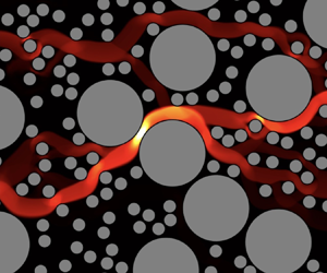
Figure 5. Channelisation characteristics: (a) schematic illustration of  $L_{ch}$ and $h_{ch}$ definition; (b) velocity contour for $\phi =0.5$ and $B=10^4$; (c) velocity contour for $\phi =0.1$ and $B=10^4$.
In our recent study (Fraggedakis et al. Reference Fraggedakis, Chaparian and Tammisola2021), we have shown that the mean height of the first open channel scales with the porosity, i.e.  $\langle h_{ch} \rangle \sim 1-\phi$ and the mean relative length of the first channel scales with the volume fraction, i.e. $\langle L_{ch} \rangle /L \sim \phi$, where $\langle {\cdot } \rangle$ stands for the mean quantity which is acquired by ensemble averaging through different simulations and also various porosities. To elaborate, in a condensed system of obstacles (i.e. low porosities), $h_{ch}$ is smaller since the fluid path is squeezed between the obstacles or the mean void length between the obstacles becomes smaller as the solid volume fraction increases. On the other hand, the mean relative length of the first channel or tortuosity (i.e. $L_{ch}/L$) scales with the solid volume fraction since in a denser system, the minimum path's shape is a zigzag rather than straight, which is more probable in a more dilute system of obstacles. These interpretations are evidenced in figure 5 by sample illustrations: figure 5(b) shows a sample simulation for $\phi =0.5$ in which the first channel is very thin and long compared with figure 5(c) in which $\phi =0.1$ and the channel is rather thick and straight ( $L_{ch} \to L$).
Inserting the scales for the mean height and the mean relative length of the first channel to expression (4.4), the critical yield number can be re-written as
 \begin{equation} Y_c \sim \frac{\left\langle h_{ch} \right\rangle}{\left\langle L_{ch} \right\rangle/L} \sim \frac{1-\phi}{\phi} \equiv \frac{\text{Void space}}{\text{Obstructed space}}, \end{equation}
which means that the critical yield number scales with the ratio of the void space to the solid (i.e. obstructed) space.
In figure 6, we present a comparison of the theory (i.e. expression (4.5)) with the data associated with the simulations performed in the current study and also the previously published data: the non-dimensional critical pressure gradient (i.e.  $1/Y_c$) is plotted versus $\phi /(1-\phi )$. The dashed orange line is the scale derived above, i.e. expression (4.5). The hollow symbols are the present computed data: black and purple colours are denoted to monodispersed and bidispersed cases, respectively. Circles, squares and pentagrams represent the circle, square and polygon obstacles, respectively. The filled circle symbols with the uncertainty bars are the data borrowed from Fraggedakis et al. (Reference Fraggedakis, Chaparian and Tammisola2021) where a pore-network approach is utilised to analyse a large number of realisations ( $\sim 500$ for each porosity) with circular obstacles where each colour represents a specific $\hat {R}/\hat {L}$ ratio. Indeed, the filled circle symbols are the ensemble averages of all previously performed simulations and the uncertainty bars represent the range of obtained values. For more clarification of the used data, please see Fraggedakis et al. (Reference Fraggedakis, Chaparian and Tammisola2021). However, as explained in § 2.3, the current data is acquired through individual simulations (i.e. they are not ensemble averages of many simulations), hence, no uncertainty bars are associated with the new data (i.e. hollow symbols).

Figure 6. Comparison between our theory and the computational result: non-dimensional critical pressure gradient versus  $\phi /(1-\phi )$. The dashed orange line is the scale derived in (4.2). The filled circle symbols with uncertainty bars are the data borrowed from Fraggedakis et al. (Reference Fraggedakis, Chaparian and Tammisola2021). Each colour intensity is dedicated to a different value of $\hat {R}/\hat {L}$ between 0.02 to 0.1 (see the reference for more details). The black and purple hollow symbols denote the monodispersed and bidispersed cases, respectively. Circles, squares and pentagrams represent the circle, square and polygon obstacles, respectively. Inset: comparison between the upper bound of the critical pressure gradient (cyan line) derived by Castañeda (Reference Castañeda2023) and the proposed universal scale (dashed orange line). Please note that the axes of the inset are the same as the main figure.
A reasonable agreement can be observed between the derived scale (with a fitted slope  $\approx 3.14$ or ${\rm \pi}$) and the computational data for all class of considered topologies. Moreover, the bidispersed cases data also fits reasonably to the proposed theory.
In a very recent study, using a ‘variational linear comparison’ homogenisation method, Castañeda (Reference Castañeda2023) has derived an upper bound for the critical pressure gradient where the solution of Newtonian fluids is used as a test function in the dissipation-rate potential of viscoplastic fluids. This upper bound is shown by the cyan line in the inset of figure 6 along with the proposed universal scale for comparison. Note that the upper bound proposed by Castañeda (Reference Castañeda2023) has a linear functionality with  $\phi / (1-\phi )$ which further validates the universal scale derived here, although its slope is steeper – which is not surprising as it is an upper bound.
5. Concluding remarks
Adaptive finite element simulations based on an augmented Lagrangian scheme were performed to study the fluid flows of yield-stress fluids in porous media. The specific objective was to fully understand the yield limit of this type of flow and propose a theory to address the critical applied pressure gradient which should be exceeded for flow assurance purposes. This is a vital and a very base step in proposing a generic Darcy type expression for bulk transport properties of the yield-stress fluid flows in porous media.
For this aim, and to avoid prevailing analysis, flows in various porous media constructed with a wide range of obstacle shapes are investigated. The studied geometries have been generated by randomly distributing non-overlapping obstacles of circular and square shapes. In addition, more complicated topologies (i.e. polygon obstacles), have been generated by using the Voronoi tessellation of circular cases. The computational data includes both monodispersed and bidispersed systems.
In the yield limit, which is the main focus of the present study, the flow is restricted to a single channel connecting the inlet to the outlet, while the fluid outside of it is unyielded and thus quiescent. The configuration of this very first channel has been investigated in our previous study (Fraggedakis et al. Reference Fraggedakis, Chaparian and Tammisola2021) and statistical geometrical properties (e.g. height and length) are reported as a function of the solid volume fraction ( $\phi$) or alternatively the porosity of the domain ( $1-\phi$) which can be summarised as $\langle h_{ch} \rangle \sim 1-\phi$ and $\langle L_{ch} \rangle / L \sim \phi$.
A theory was proposed based on variational formulation of the energy equation. The leading-order plastic dissipation has been approximated by a channel Poiseuille flow at the yield limit where the channel dimensions are borrowed from the discussed statistical results (Fraggedakis et al. Reference Fraggedakis, Chaparian and Tammisola2021). Indeed, in the very first channel, the transport mechanism is predominantly postulated by the core unyielded plug in the middle of the channel and the leading-order plastic dissipation occurring in the sheared boundary layer between the quiescent fluid outside of the channel and the mobilised core unyielded region. It should be noted that due to the complex shape of this limiting channel in the porous media, the mechanism is not as simple as explained above since the limiting channel is not straight and channel height varies (especially in the dense systems), see figure 5. Thus, the core unyielded plug and the adjacent boundary layers are not uniform. Nevertheless, since the mean height and length of the channel is used in our model, the proposed scaling is still valid in the leading order. This has been assessed using the obtained computational data for a wide range of obstacle topologies mentioned above and also previously published data. We have shown that our theoretical approach is capable of predicting the numerical data with a reasonable agreement.
Due to the high cost of unregularised numerical simulations of yield-stress fluid flows and also handling various shapes of obstacles, the available data, especially in the yield limit, is limited. This limitation is more evident in three-dimensional flows. Although in some studies (Bittleston, Ferguson & Frigaard Reference Bittleston, Ferguson and Frigaard2002; Pelipenko & Frigaard Reference Pelipenko and Frigaard2004; Hewitt et al. Reference Hewitt, Daneshi, Balmforth and Martinez2016; Izadi et al. Reference Izadi, Chaparian, Trudel and Frigaard2023), the Hele-Shaw approximation for yield-stress fluids has been developed, still the lack of a compelling study linking this pore-scale approximation to bulk transport mechanisms/features in three dimensions is evident. This is left for future investigations, both theoretically and computationally, which is a massive step forward for many industrial applications.
Acknowledgements
The author thanks B. Nasouri for fruitful discussions in the course of this study.
Declaration of interests
The author reports no conflict of interest.


 Open access