


Introduction
For predicting the safe bearing capacity of a floating ice sheet, the ice sheet is usually represented by the mathematical theory of a thin plate floating on the surface of the water. This theory predicts the stresses correctly when the load is distributed over a sufficiently large area, but when the load distribution becomes small, the thin-plate theory over-estimates the stresses in the vicinity of the load.
The first person to recognize this problem of incorrect stresses in the vicinity of a load distributed over a small area was Reference HertzHertz (1884). He recommended that the smallest diameter of load distribution used for stress calculations should be equal to the ice thickness.
When the load is distributed over a circular area, Reference WestergaardWestergaard (1926) presented a formula for the maximum stress which occurs at the bottom of the plate directly under the center of the load. His formula was based on the solution of a three-dimensional elastic layer which was developed by Reference NadaiNadai (1920, see also Reference NadaiNadai 1925, p. 308). Nadai considered a finite, axially-symmetrical, elastic layer whose bottom surface was free of stresses and whose top surface had a normal load, uniformly distributed over a circular area. The circumferential boundary corresponded closely to that of a simple support in thin-plate theory. Westergaard evaluated this solution for the maximum stress when the radius of the load was five times the thickness of the layer. When the radius of the load was greater than 1.724 times the layer thickness, he found that the thin-plate theory gave the same stress as the three-dimensional theory. When the radius of the load was less than 1.724 times the layer thickness, he found a difference between the two theories. He then stated that the thin-plate theory could still be used provided a fictitious load radius is used. The fictitious radius a was given by
where b is the true load radius and h is the ice thickness. Approximately the same results were obtained with layers whose radius-to-thickness ratios were other than five. Westergaard then stated, “The results may be applied generally to slabs of proportions such as are found in concrete pavements, with any kind of support which is not concentrated within a small area close to the load”.
Reference Woinowsky-KriegerWoinowsky-Krieger (1933) developed the three-dimensional elastic-layer solutions in rectangular and radial coordinates for loads distributed over rectangular and circular areas respectively. He presented numerical results for the maximum tensile stresses in a simply-supported and a clamped-supported axially symmetrical elastic layer without an elastic foundation. Woinowsky-Krieger also developed equations for the deflection of plates on an elastic foundation, but he did not discuss the stresses.
Reference NevelNevel (1970) considered the stresses at the bottom of the ice sheet directly under the center of a load uniformly distributed over a circular area. He used elastic-layer theory and this theory gave the same numerical results as Westergaard’s “fictitious" radius method. However, the stresses when the radial coordinate r was not zero were not evaluated.
It is the purpose of this paper to develop and evaluate these stresses when the radial coordinate is non-zero as well as zero. These results are important for the superposition of stresses when two concentrated loads act near each other. In addition, the equations for a rectangular load will be developed and evaluated.
Circular Loads
Consider an ice sheet of uniform thickness floating on the surface of the water. Assume that the horizontal extent of the ice sheet is sufficiently large that we may assume the ice sheet extends to infinity in any horizontal direction. Let a load which is uniformly distributed over a circular area be applied vertically to the top surface. The increase in vertical pressure on the bottom surface due to the applied load will be equal to the unit weight of water times the vertical deflection of the bottom surface. The shearing stresses on both the top and bottom surfaces are zero.
Reference NevelNevel (1970) has solved this problem when the ice sheet is considered as a three-dimensional elastic layer. His method of solution for this axially symmetrical problem consisted of using a Hankel transform with respect to the radial coordinate. This method corresponds to using a Fourier transform with respect to x and y coordinates when axial symmetry occurs. From his results the stresses in the ice at the bottom surface of the ice are

and

where
In these equations ᓂr is the radial stress, ᓂᎾ is the tangential stress, P is the total load, v is Poisson’s ratio for ice, h is the ice thickness, B is b/h, b is the radius of the load distribution, R is r/h, r is the radial coordinate, H is h/l, l 4 is Eh 3[12k(I -v 2)], E is Young’s modulus for ice, k is the unit weight of water, and t is the Hankel transform parameter for R.
Typical values of H are between 0.01 and 0.1 for ice sheets floating on water. Hence it can be shown that the H 4 terms in the numerator of F ±p (Equation (4)) produce negligible results when compared to results from the 12t 2sinh t term. Hence, in place of F ±p we may use F where
If thin-plate theory is used to represent the ice sheet, the formulas for the stresses are the same as Equations (2) and (3) except that now the F function becomes
Consider the stresses directly under a concentrated load, R = B = 0. For the stress sum ᓂᎾ+ᓂr, the integrand becomes F times t. For plate theory, F p times t is approximately 3/t for very large t. Hence, the ᓂᎾ+ᓂr integral diverges for plate theory when R = B = 0. For elastic layer theory, F from Equation (5) is 3t 2/(t 4+H 4) when t is small, which is the same as Fp. If we factor 3t 2/(t 4+H 4) out of F, the remaining factor is the additional factor of the elastic-layer solution which does not appear in the plate solution. This additional factor is shown in Figure 1, and, for H 0.1, it is nearly independent of H. This additional factor becomes 2t 3 exp (-t)/3 for large t, which provides convergence for the ᓂ0 + ᓂr integral when t goes to infinity.
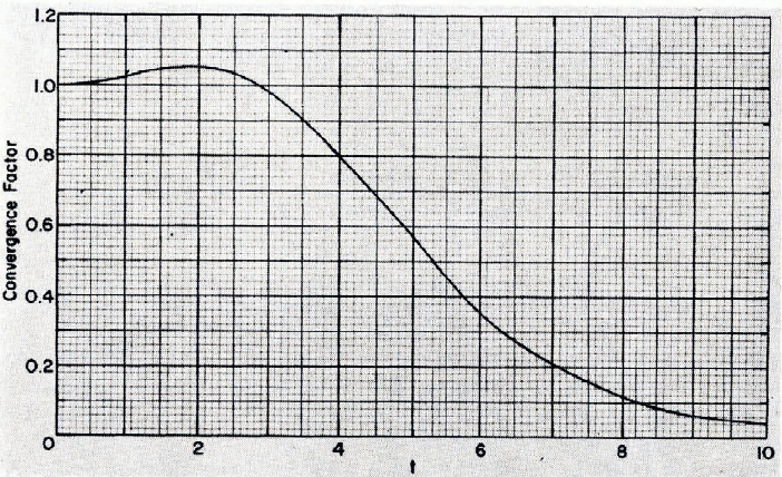
Fig. 1. Convergence factor.
In order to perform the integration for ᓂᎾ+ᓂr in Equation (2) when R = B = 0, the integration is divided into regions. In the region from t = 0 to t = 2, the convergence factor is expanded into a series about t = 0 and the integration performed. In the region from t = 2 to t = ∞, the integration can be performed after the integrand has been expanded into an asymptotic series. The result is
where the zero superscript designates R = B = 0.
Let us now subtract (ᓂᎾ + ᓂr)°from ᓂᎾ+ᓂr. Using a superscript star to designate this difference, we have

The factor F in the integrand depends on H only near t = 0, while the factor J 0 (tR) J 1 (tB)/(tB/2) - 1 is very small near t = 0. Hence, one might suspect that the integral of the product may be nearly independent of H. When H = 0, F becomes
In order to estimate the error in using F 0 in Equation (8) rather than F, consider

where the subscript e represents the error of neglecting H. Since F-F 0 is zero except near t = 0, we can expand the Bessel function into a series about t = 0. Retaining only the first significant term we integrate to obtain
Let us now consider the stress difference ᓂ0-ᓂr of Equation (3). The factor J1(tR)/(tR/2)-J0(tR) of the integrand is small near t = 0, and hence, one might suspect again that the integral is nearly independent of H. We can estimate the error of neglecting H by considering F-F 0. Proceeding as before we get
Equations (11) and (12) were compared with results obtained from numerical integration and the error was less than 0.000 1 when H = 0.1, B = 2, and R = 3. The error is even less when H, B, or R is less than the stated values.
Hence we can now consider the stresses of Equations (3) and (8) using F 0 rather than F, which makes the integrals independent of H. The integrals were numerically integrated in steps of 0.01 from t = 0 to t = 10 by means of Simpson’s quadrature. Results were obtained when the radial coordinate R was varied in steps of 0.1 from 0 to 3 while the radius of the load distribution was varied in steps of 0.1 from o to 2. The results for (ᓂ0+ᓂr)* are shown in Figure 2. To this result must be added Equations (7) and (11) to obtain the total ᓂ0+ᓂr. The results for ᓂ0—ᓂ r are shown in Figure 3. To this result must be added the solution of Equation (12) to obtain the total ᓂ0—ᓂr.

Fig. 2. Stress sum as a function of B and R.
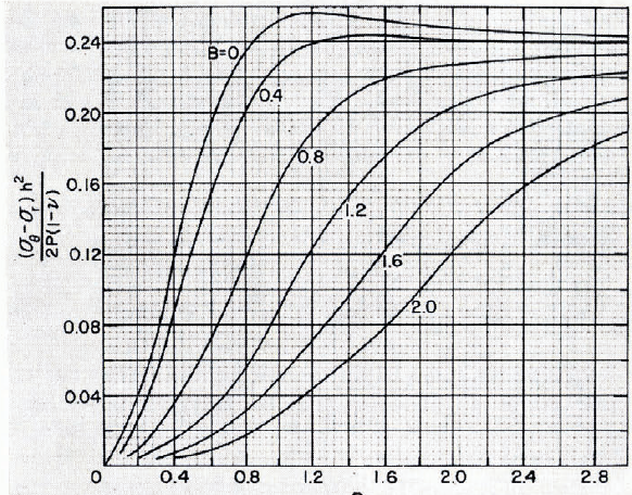
Fig. 3. Stress difference as a function of B and R.
At a sufficiently large R, the elastic-layer theory and the thin-plate theory should predict the same results. One would expect the greatest difference between these theories when B = 0. Table I shows the difference between these two solutions as functions of R.
TABLE I. ELASTIC-LAYER THEORY MINUS PLATE THEORY

Rectangular Loads
The solution for a load uniformly distributed over a rectangular area is obtained in a similar manner as for a circular load. The difference being that now Fourier transforms with respect to x and y are utilized rather than a Hankel transform with respect to r. Since the general method of solution has been previously given by Reference Woinowsky-KriegerWoinowsky-Krieger (1933), it will not be repeated here. The stresses at the bottom of the ice sheet are


and

where all notations are the same as for the circular load except that now ᓂx is the stress in the x direction, ᓂy is the stress in the y direction, ᓂxy is the shear stress in the x-y plane, X is x/h, x is the x coordinate, Y is y/h, y is the y coordinate, A is a/h, a is the half-length of the load distribution in the x direction, B is b/h, b is the half-length of the load distribution in the y direction, α is the Fourier transform parameter for X, β is the Fourier transform parameter for Y, and t z is α2+β2. The solution for a rectangular load using thin-plate theory is given by Equations (13), (14) and (15) provided F ±v is replaced with F p. As in the circular load case, we may neglect the H 4 terms in the numerator of F ±v, and replace F ±v with F. For a concentrated load at x = y = 0, ᓂx - ᓂy and ᓂxy are zero while ᓂx+ᓂy gives the same result as ᓂ0+ᓂr.
In order to reduce the effect of H on ᓂx+ᓂy, let us subtract the concentrated load solution at x = y = 0. Designating this difference with a superscript star, we have

As in the circular-load case, we suspect that the integrals of Equations (14), (15), and (16) are relatively independent of H. An estimate of the error for neglecting H in F for these integrals can be made by replacing F with F-F 0. Expanding the sines and cosines into a series and proceeding as before we obtain
Hence, we can now consider the stresses of Equation (14), (15), and (16) using F 0 rather than F, which makes the integrals independent of H. However, the solutions are still a function of the load distribution A and B as well as the coordinates X and Y. In order to reduce the number of parameters to a manageable level, let us consider the stresses directly under the center of the load at X = Y = 0. For this case ᓂxy = 0. The other two integrals were numerically integrated in steps of 0.1 from α = 0 to α = 10 and in steps of 10 from β = 0 to β = 10 by means of Simpson’s quadrature in two variables. The load distribution distance B was varied in steps of 0.1 from 0 to 3 while the ratio A/B was varied in steps of 0.2 from o to 1. The result for (ᓂx+ᓂy)* is shown in Figure 4. Interchanging A and B does not change the value of (ᓂx+ᓂy)*. The result for ᓂx—ᓂy is shown in Figure 5. Interchanging A and B changes the sign of ᓂx—ᓂy

Fig. 4. Stress sum at X = Y = 0 as a function of B and A/B.
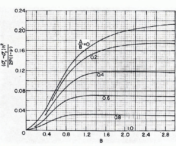
Fig. 5. Stress difference at X = Y = 0 as a function of B and A/B.
Conclusions and Recommandations
The stresses in the vicinity of a relatively concentrated load have been determined for loads distributed over both circular and rectangular areas by using elastic-layer theory. This corrects the deficiency of overestimating these stresses created by thin-plate theory.
Although the problem has been solved, it still would be desirable to develop a more convenient algorithm of computation than straight numerical integration. One approach would be to use approximation functions. For example, the approximation
seems to work reasonably well if B and R are not too large.
Another more rational approach would be to develop the integrand into a series and integrate. However a power series development does not work. More hopeful is to develop the integrand into a Bessel-function series and integrate each term by means of contour integration. This method, although rather complicated may produce a better computation algorithm.
Discussion
L. LLIBOUTRY: All your calculations assume perfect elasticity. Have you done any calculations taking creep (especially transient creep) into account?
D.E. NEVEL: Yes. This work has been described in another recent report of mine Reference Nevel(Nevel, 1976).
E. VITTORATOS: One practical problem with Bessel-function expansions would be that these functions are not available in pre-programmed form in calculators or micro-processors; one generally needs a rather large computer.
NEVEL: Usually in bearing-capacity problems the arguments of the Bessel functions are not too large. Hence a series expansion is an efficient method of computation. In the case of the modified Bessel functions (ber, bei, ker, kei), the computational method of using a recurrence relation between the different functions and their derivatives Reference Nevel(Nevel, 1959) is efficient in terms of computer space and time. The “safe" bearing capacity program of CRREL utilizes this method in a subroutine. The computation is done on a desk-top calculator, the Hewlett-Packard 9820. There are some new hand-held calculators, such as the HP-67, in which I believe this computer program can be made to work. The real computational problem appears to be with the Fourier-series solutions which occur when rectangular coordinates are used. The series are slowly convergent when the arguments are small. The method of expanding the sines and cosines into a Bessel series and integrating by contour methods may provide a more convergent series which would solve this problem.


