


1. Introduction
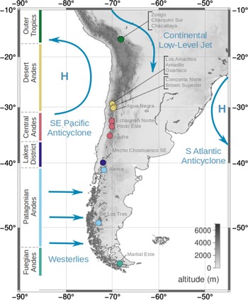
A large fraction of southern hemisphere glaciers is located in the Andes of South America (Pfeffer and others, Reference Pfeffer2014). Due to the Andes’ high latitudinal and altitudinal range, its glaciers are situated in very different climatic conditions (Sagredo and Lowell, Reference Sagredo and Lowell2012). The northern section of the mountain range is subjected to a tropical climate, the subtropics of South America are hosting one of the driest regions on Earth, and the mid latitudes are humid and dominated by frontal systems (Fig. 1; Garreaud and others, Reference Garreaud, Vuille, Compagnucci and Marengo2009). Consequently, the Andes cover a broad range of glaciological regimes, and glaciers react differently to climatic disturbances (Sagredo and others, Reference Sagredo, Rupper and Lowell2014, Reference Sagredo2017).
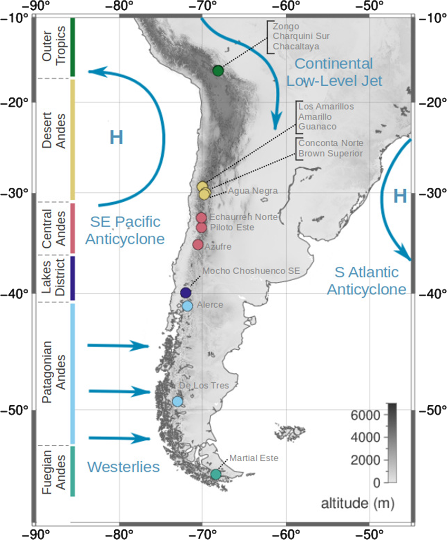
Fig. 1. Overview of South American climatic conditions (dark blue) and the locations (circles) and geographic classifications (circle colours) of the glaciers in this study. The glaciers are categorised with respect to prevailing regional geographic conditions. These categories are largely based on the glaciological zones proposed and used by Lliboutry (Reference Lliboutry1998), updated by Barcaza and others (Reference Barcaza2017), and Zalazar and others (Reference Zalazar2020).
South American glaciers follow the recent general trend of glacial retreat that is monitored worldwide (WGMS, 2017). Environmental and socioeconomic consequences of this development are manifold. Although mountain glaciers only hold ~ 0.12 % of the global freshwater resources, they play an important role in the global water cycle and regional water management (Shiklomanov, Reference Shiklomanov1993). In regions such as the Dry Andes, where precipitation is concentrated in winter months, glaciers act as a freshwater reservoir in dry seasons (e.g. Kaser and others, Reference Kaser, Juen, Georges, Gómez and Tamayo2003; Favier and others, Reference Favier, Falvey, Rabatel, Praderio and López2009; Kaser and others, Reference Kaser, Großhauser and Marzeion2010; Burger and others, Reference Burger2019). With a changing climate and accompanying ice mass loss in the Andes, this runoff smoothing effect is diminished and the point of maximum runoff has possibly been passed already (Ragettli and others, Reference Ragettli, Immerzeel and Pellicciotti2016; Huss and Hock, Reference Huss and Hock2018). Furthermore, hydroelectric power supply, agricultural irrigation, water for human consumption and industrial processes can no longer be guaranteed in some areas in the future in case of the disappearance of Andean glaciers (Vergara and others, Reference Vergara2007). The receding of Patagonian glaciers may additionally lead to a decrease in local tourism and economy due to their value as tourist attractions (Vergara and others, Reference Vergara2007). Case studies of the Cotacachi glacier in Ecuador demonstrate how the disappearance of a glacier already results in a decline in agriculture, tourism and biodiversity in surrounding areas (Rhoades and others Reference Rhoades, Ríos and Aragundy2006; Vergara and others, Reference Vergara2007). About half of the global human population lives in coastal areas, making sea level rise one of the potentially most severe consequences of contemporary climate change (Leatherman, Reference Leatherman2001; Douglas and others, Reference Douglas, Kearney and Leatherman2001). Although mountain glaciers make up only a relatively small fraction of stored solid water on Earth compared to the ice sheets of Greenland and Antarctica, mountain glaciers are estimated to contribute 25–30% to the observed sea level rise in the period 1961–2016 due to faster reactions to the changing climate (Meier, Reference Meier1984; Kaser and others, Reference Kaser, Cogley, Dyurgerov, Meier and Ohmura2006; Zemp and others, Reference Zemp2019; IPCC, 2021). The total water stored in the glaciers of the Southern Andes represents a mean sea level equivalent of ~ 13 mm (Stocker and others, Reference Stocker2013; Farinotti and others, Reference Farinotti2019) and ice volume of ~ 5.34 ± 1.39 · 103 km3 (Farinotti and others, Reference Farinotti2019).
The above described observed and potential consequences of glacial retreat stress the need for accurate model-based predictions of mountain glacier mass-balance changes to allow for more informed mitigation strategies and policy making. Additionally, glacier modelling can provide insights into past climate conditions and complement palaeoclimate modelling and dating of past glacial geometries (Hostetler and Clark, Reference Hostetler and Clark2000; Hulton and others, Reference Hulton, Purves, McCulloch, Sugden and Bentley2002; Kull and others, Reference Kull, Hänni, Grosjean and Veit2003). Finally, model-based estimates of the evolution of mountain glaciers in the geologic past can provide insight into their erosional capacity and potential impact on mountain building processes (Egholm and others, Reference Egholm, Nielsen, Pedersen and Lesemann2009; Thomson and others, Reference Thomson2010) and thus complement ongoing research of the interactions between tectonics, climate and Earth surface processes in mountain regions (e.g. Mutz and Ehlers, Reference Mutz and Ehlers2019).
Several approaches to model glacier mass-balance have been applied to glaciers in South America. These include techniques from the super-categories of empirical and physical (process-based) models. The spatial coverage of studies ranges from single glaciers to continental scale assessments of glacier changes (Fernández and Mark, Reference Fernández and Mark2016). Dynamical, numerical mass-balance models describe and parameterise physical processes on a glacier. Atmospheric variables, such as precipitation and temperature, are used as boundary conditions. These models are commonly classified by their implementation of ablation processes: Degree day models estimate the surface mass loss on a glacier on a daily basis using temperature (e.g. Tangborn, Reference Tangborn1999), while energy-balance models capture ablation processes based on radiation, longwave fluxes, sensible and latent heat (e.g. Oerlemans, Reference Oerlemans1992). More sophisticated models calculate the energy budget on a glacier by including parameters such as humidity, pressure, snowdrift, snowpack evolution and runoff processes in addition to temperature and precipitation (Oerlemans, Reference Oerlemans1993; Mernild and others, Reference Mernild, Liston, Hiemstra and Wilson2017). These models typically have tuning parameters that need to be derived empirically with measurements of mass-balance and climate elements. Therefore, the above described models rely on fine-scaled atmospheric data in the vicinity of the glacier. When coupling these glacier models to the relatively coarse output of general circulation models (GCMs), climate simulations have to be downscaled first to fit the needs of the mass-balance model (e.g. Reichert and others, Reference Reichert, Bengtsson and Oerlemans2001; Schaefer and others, Reference Schaefer, Machguth, Falvey and Casassa2013; Mernild and others, Reference Mernild, Liston, Hiemstra and Wilson2017). The two main downscaling approaches are numerical and empirical-statistical downscaling (ESD) (for a review on downscaling strategies, see Giorgi and others, Reference Giorgi2001). Numerical downscaling uses an approximation for underlying physical processes in order to make predictions of regional weather conditions based on a larger-scale atmospheric state. ESD uses empirical-statistical relationships of local-scale meteorological measurements and large-scale climate patterns (Wilby and others, Reference Wilby2004). ESD-based modelling assumes the temporal stationarity of these relationships. When driving glacier models with downscaled climate conditions, uncertainties introduced in the downscaling process are potentially propagated in the modelling of glacier mass-balance and add another layer of uncertainty to the uncertainties of capturing complex physical processes of a glacier.
Alternatively, one can employ statistical techniques (e.g. Hoinkes, Reference Hoinkes1968; Lliboutry, Reference Lliboutry1974; Condom and others, Reference Condom, Coudrain, Sicart and Théry2007) or apply a modification of the ESD approach directly on the glaciers to estimate changes in their mass-balance (e.g. Schöner and Böhm, Reference Schöner and Böhm2007; Mutz and others, Reference Mutz, Paeth and Winkler2015). In such a procedure, glacier mass-balance replaces local atmospheric variables as the prediction target (predictand), thus circumventing the costly intermediate step of climate downscaling. Since local geographic conditions are implicitly included in empirical models, it also removes the need to explicitly parameterise those for the location of the investigated glaciers. This approach requires sufficiently long and temporally overlapping measurements of atmospheric predictors and glacier mass-balance in order to adequately capture robust empirical transfer functions between them. Furthermore, it requires knowledge of glacier-climate interactions in the region to ensure that physically meaningful predictors are chosen and captured empirical relationships represent underlying physical processes. The growing South American mass-balance record lends itself to this approach, and previous studies of relationships between atmospheric quantities and South American glaciers (Sagredo and Lowell, Reference Sagredo and Lowell2012; Mernild and others, Reference Mernild2015; Maussion and others, Reference Maussion, Gurgiser, Großhauser, Kaser and Marzeion2015; Veettil and others, Reference Veettil, Bremer, de Souza, ÉLB and Simões2016) allow for a well-informed selection of predictors. While some studies have used an empirical approach on a small selection of glaciers in South America (Manciati and others, Reference Manciati2014; Maussion and others, Reference Maussion, Gurgiser, Großhauser, Kaser and Marzeion2015), none have taken full advantage of available mass-balance records to assess mass-balance changes in context of synoptic-scale climate and generate future estimates across South America.
In this study, an ESD approach is applied to a selection of Andean glaciers south of 15°S. ESD-based empirical glacier mass-balance models (EGMs) are trained for individual glaciers. They capture the transfer functions between glacier mass-balance variations and large-scale climate variability obtained from ERA-Interim reanalysis. In order to demonstrate the application of such models, the EGMs are then coupled to simulations of the Max-Planck-Institute's Earth System Model (MPI-ESM-MR) of the Coupled Model Intercomparison Project (CMIP5) to estimate the mass-balance response to potential future climate change under different greenhouse gas (GHG) concentration scenarios (see Supplementary material). The following goals are addressed by this study:
• To identify synoptic-scale atmospheric predictors of South American glacier mass-balance and quantify their influence.
• To assess the potential of an ESD-based modelling approach for South American glacier mass-balance.
• To generate, evaluate and apply EGMs for each Andean glacier that is suitable for an ESD-based modelling approach.
2. Data and methods
2.1 Glaciers in South America
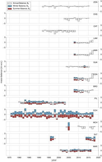
The response of glacier front variations to external forcing depends on topography and glacier size, and can result in time lags of up to several years (Müller, Reference Müller1987; Jóhannesson and others, Reference Jóhannesson, Raymond and Waddington1989; Cuffey and Paterson, Reference Cuffey and Paterson2010). Therefore, glacier extent and frontal variation are not well suited for statistical mass-balance models (Hodge and others, Reference Hodge1998) and the models in this study are trained with glacier-wide mass-balances based on observational records constructed with the glaciologic method described in Braithwaite (Reference Braithwaite2002). These data are provided by the World Glacier Monitoring Service (WGMS) database (WGMS, 2018). Due to the requirements of the ESD approach, our first selection of glaciers restricted to those with annual mass-balance (Ba) records covering at least 10 years in succession. Eleven South American glaciers fulfill these requirements. They are located in a latitudinal range of 16 °S to 55 °S and different climatic and glaciological zones (Fig. 1, Lliboutry (Reference Lliboutry1998), updated by Barcaza and others (Reference Barcaza2017), and Zalazar and others (Reference Zalazar2020)). Five additional glaciers, Agua Negra (AGN), Azufre (AZF), Alerce (ALC), Mocho Choshuenco SE (MCH) and De Los Tres (DLT), are included in our study to increase the number of representatives for South American glaciological zones. Our study thus considers glaciers of the Outer Tropics (Zongo (ZON), Charquini Sur (CHS), Chacaltaya (CHT)), Desert Andes (Los Amarillos (LAM), Amarillo (AMA), Guanaco (GUA), Conconta Norte (CON), Brown Superior (BRO) and AGN), Central Andes (Echaurren Norte (ECH)), Piloto Este (PIL and AZF), Lakes District (MCH), Patagonian Andes (ALC and DLT) and Fuegian Andes (Martial Este (MAR)). The mass-balance records for MCH and DLT are sufficiently long to include them in our analyses computationally despite not meeting the procedures’ requirements listed above. Glacier names, acronyms, geographical setting and record length are summarised in Table 1. Overviews of annual and seasonal mass-balance changes and recent cumulative mass loss are provided in Figures 2 and 3 respectively. Mass-balance data are given in units of meters water equivalent (m w.e.), i.e. the mass change per unit area divided by the density of water (Cogley and others, Reference Cogley2011).

Fig. 2. Glacier mass-balance records used in this study. Annual mass-balance (Ba) is shaded in grey, winter mass-balance (Bw) is shaded in blue, and summer mass-balance (Bs), the difference between Ba and Bw, is shaded in red. For some glaciers, only annual data exist. Notable differences in mass turnover can be observed for the glaciers with seasonal mass-balance data.

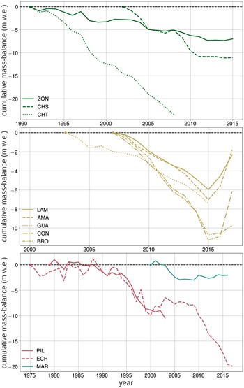
Fig. 3. Cumulative annual mass-balances of the glaciers used in this study. The cumulative balances are set to zero at the beginning of the measurement for each record. Colour coding corresponds to the glaciological zones presented in Figure 1.
Table 1. Names, acronyms, geographical position, elevation range, area, setting and number of available mass-balance measurements (annual mass-balance (Ba), winter mass-balance (Bw) and summer mass-balance (Bs)) for each glacier used in this study (until mid-2019)

Elevation (m.a.s.l.) is provided as a minimum to maximum range in the observed period. The zones are consistent with those of Figure 1.
2.2 ERA-Interim reanalysis
ERA-Interim reanalysis data of the European Centre for Medium-Range Weather Forecast (ECMWF) (Berrisford and others, Reference Berrisford2011) is a global, homogenous dataset compiled with a data assimilation scheme which combines local observations of the atmospheric state with a dynamical numerical model. This scheme allows interpolations of observations in a physically consistent way (Dee and others, Reference Dee2011). The dataset covers the period from 1979 onward and is updated regularly in real time (Berrisford and others, Reference Berrisford2011). Data assimilation is done in 60 vertical model levels from the land surface up to the 0.1 hPa pressure level (Dee and others, Reference Dee2011). The model output of the reanalysis is interpolated onto a 0.75° × 0.75° native longitude-latitude grid. At the equator, this roughly represents a 80 km x 80 km grid spacing (Dee and others, Reference Dee2011). Monthly averages of daily mean values of the ERA-Interim dataset are used to calculate predictors for the mass-balance modelling (see Predictor construction section).
2.3 Empirical-statistical glacier mass-balance models
2.3.1 Predictor construction
Potential predictors for empirical mass-balance modelling are chosen on the basis of their physical relevance to glacier mass-balance changes. More specifically, the criteria for consideration is the predictors known ability to alter surface energy balance, accumulation or other processes that influence the mass-balance of mountain glaciers. Additionally, the predictors should be adequately represented in GCMs to merit the EGM-GCM coupling.
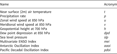
Local precipitation and temperature are the main direct controls for accumulation and ablation respectively (Oerlemans and Reichert, Reference Oerlemans and Reichert2000; Sagredo and others, Reference Sagredo, Rupper and Lowell2014). We therefore use synoptic-scale atmospheric variables that are known to be good predictors for regional temperature and precipitation (Huth, Reference Huth2002; Cavazos and Hewitson, Reference Cavazos and Hewitson2005; Garreaud and others, Reference Garreaud, Lopez, Minvielle and Rojas2013; Mutz and others, Reference Mutz, Scherrer, Muceniece and Ehlers2021). Statistical temperature downscaling should include at least one predictor reflecting temperature and one circulation-related predictor (Huth, Reference Huth2002). Suitable predictors for precipitation downscaling are mid-tropospheric geopotential height, humidity (Cavazos and Hewitson, Reference Cavazos and Hewitson2005) and dew-point temperature depression (Charles and others, Reference Charles, Bates, Whetton and Hughes1999). We also include zonal and meridional wind component at 850 hPa level and the Antarctic Oscillation (AAO) due to their known control on precipitation in Patagonia (Silvestri and Vera, Reference Silvestri and Vera2003; Garreaud and others, Reference Garreaud, Lopez, Minvielle and Rojas2013). Inclusion of the latter is also supported by its correlation with mass-balance variation in the Peruvian Andes (Kaser and others, Reference Kaser, Juen, Georges, Gómez and Tamayo2003). Furthermore, several studies suggest a significant influence of El Niño-Southern Oscillation (ENSO) on Andean low-latitude glaciers (Ribstein and others, Reference Ribstein, Tiriau, Francou and Saravia995; Kaser and others, Reference Kaser, Juen, Georges, Gómez and Tamayo2003; Francou and others, Reference Francou, Vuille, Favier and Cáceres2004; Rabatel and others, Reference Rabatel2013; Maussion and others, Reference Maussion, Gurgiser, Großhauser, Kaser and Marzeion2015; Veettil and others, Reference Veettil, Bremer, de Souza, ÉLB and Simões2016), and a relationship between the Pacific Decadal Oscillation (PDO) and glacier fluctuation for tropical glaciers of the Andes (Veettil and others, Reference Veettil, Bremer, de Souza, ÉLB and Simões2016). Indices for both are also included in our set of potential predictors. The complete set of potential predictors thus comprises indices of the AAO, ENSO and PDO, as well as regional means of 2m air temperature (t), precipitation (p), mean sea level pressure (slp), zonal wind speed at 850 hPa (u), meridional wind speed at 850 hPa (v), dewpoint temperature depression at 850 hPa (dpd) and geopotential height at 700 hPa (h). The predictors are calculated as annual and seasonal values. In this study, seasons refer to times of accumulation (April–September) and ablation (October–March).
The regional means that serve as predictors are anomalies of spatial averages that are obtained by averaging the grid points within a 500 km radius around each glacier. An overview on methods to calculate an index of the AAO (aaoi) is given in Ho and others (Reference Ho, Kiem and Verdon-Kidd2012). We adopt the method of the National Oceanic and Atmospheric Administration (NOAA) based on empirical orthogonal function (EOF) analysis (NOAA, 2005): The monthly mean 700 hPa height anomaly field south of 20 °S is projected onto the loading pattern of the AAO. The loading pattern is the first mode of variability obtained by EOF analysis over the monthly mean 700 hPa height field poleward from 20 °S. The seasonal cycle is removed from the data before performing the EOF analysis. In order to account for a spherical Earth, the gridded climate data are weighted by the square-root of the cosine of latitude. An index of the PDO is obtained in a similar way. Sea surface temperature anomalies north of 20 °N are projected onto the loading pattern of the Pacific Decadal Oscillation Index (pdoi) (Garreaud and others, Reference Garreaud, Vuille, Compagnucci and Marengo2009). The loading pattern is obtained by performing an EOF analysis on the sea surface temperature anomalies north of 20 °N. We use the Multivariate ENSO Index (mei) as an index for ENSO (see Wolter and Timlin, Reference Wolter and Timlin1993, for an initial definition). The mei is constructed following Wolter and Timlin (Reference Wolter and Timlin2011) with slight modifications following Mutz and others (Reference Mutz, Scherrer, Muceniece and Ehlers2021).
2.3.2 Correlation analysis
Correlation analyses aid in the first assessment of the suitability of constructed atmospheric variables as predictors of glacier mass-balance in South America. We use the Pearson correlation coefficient (PCC), which is a common measure for linear statistical dependence of two random variables (Von Storch and Zwiers, Reference Von Storch and Zwiers2003; Wilks, Reference Wilks2006). The PCC or r is calculated for each glacier mass-balance record $\vec {y}$ and potential predictor $\vec {x}$
 as:
as:

where y i, x i are the i-th element of the i = 1, …, n elements in $\vec {y}$ and $\vec {x}$
 respectively. $\bar {y}$
 and $\bar {x}$
 are the means of the n elements in $\vec {y}$
 and $\vec {x}$
 respectively. The PCC has values between − 1 and 1 where 1 denotes a strong positive, and − 1 a strong negative linear dependence of $\vec {y}$
 and $\vec {x}$
 . We use the same equation to determine predictor multicollinearity (see Model training section). The correlation between annual and seasonal mass-balance records is determined by the same calculation performed on moving 10-year time windows (e.g. Mutz and others, Reference Mutz, Paeth and Winkler2015). The statistical significance of r is calculated with a beta distribution on the interval − 1, 1 and shape parameters a = b = n/2 − 1 (Wilks, Reference Wilks2006). The resulting value p gives an estimate on the probability that two non-related random vectors with the assumed distribution yield the same value of r (Wilks, Reference Wilks2006). We use the common significance threshold of α ≤ 0.05.
2.3.3 Model training
We construct two sets of EGMs. The models of the first set predict the annual mass-balance (Ba), while the models of the second set predict the glaciers’ mass-balance (Bw) and summer mass-balance (Bs) separately. We train the first set of EGMs for each glacier that fulfills at least the computational requirements of our approach and construct the seasonal (Bw and Bs) empirical glacier mass-balance models (EGMs) for glaciers with sufficiently long summer and winter mass-balance records. This results in a total of 13 different annual mass-balance models (for all of the study's glaciers except Agua Negra (AGN), Azufre (AZF) and Alerce (ALC)), and three winter mass-balance (Bw) and summer mass-balance (Bs) models for the glaciers Piloto Este (PIL), Echaurren Norte (ECH) and Martial Este (MAR). The EGMs are constructed by applying a classic empirical-statistical downscaling (ESD) approach (e.g. Mutz and others, Reference Mutz, Scherrer, Muceniece and Ehlers2021) directly to glacier mass-balance records, as successfully done by Mutz and others (Reference Mutz, Paeth and Winkler2015) and Schöner and Böhm (Reference Schöner and Böhm2007). The premise of this method is that the mass-balance of a glacier is linearly related to one or several variables that describe the large-scale state of the atmosphere. In its simplest form, the relationship can be summarised as:

where $\vec {Y}$ is the predictand (i.e. mass-balance), $\vec {X} = \vec {X_{1}},\; \vec {X_{2}},\; \ldots ,\; \vec {X_{p}}$
 are the predictor variables (i.e. climate variables) and ε is the remaining variance that cannot be explained by $\vec {X}$
 . The assumed linearity of the regression problem is described by:

where $\vec {a} = a_1,\; a_2,\; \ldots ,\; a_p$ are the regression model coefficients of the different predictors and b is the regression intercept. These parameters make up the core of the EGMs. Their optimal values are determined in a stepwise multiple linear regression with forward selection (Von Storch and Zwiers, Reference Von Storch and Zwiers2003). The stepwise multiple regression is performed within a k-fold cross-validation setting (Michaelsen, Reference Michaelsen1987; Zhang, Reference Zhang1993). In each fold, the data are split into training and testing subsets. The regression is conducted on the training subset, while the model's improvement is evaluated on the testing subset. Since we train our EGMs for each glacier individually, the glacier's training and testing data subsets are taken from the same glacier's mass-balance time series only. The number of folds k is set to be two-thirds of the total number of data points over which the model is fitted. From the resulting k sets of model parameters $\vec {a}$
 and b, final model parameters $\vec {\hat {a}}$
 and $\hat {b}$
 are calculated after the cross-validation. Final model parameters in $\vec {\hat {a}}$
 are computed for each parameter as arithmetic means of the k values of the cross-validation folds. In order to ensure the robustness of the model, only predictors that contributed to the improvement of the model in at least 20% of the k cross-validation folds are included in the final model. The other parameters are discarded and set to zero.
In order to reduce potential problems arising from predictor multicollinearity, predictors are pre-filtered based on a correlation analyses (see section Correlation analysis, Eqn ( 1)). For each climate variable, only the predictor time series (annual, ablation or accumulation) that is best correlated with the predictand is included in the set of potential predictors. The other two seasonal predictor time series are no longer considered. The chosen potential predictors are then correlated with each other for further filtering. If a predictor is significantly (α ≤ 0.05) or highly (with r ≥ 0.5) correlated to a predictor showing higher correlation to the predictand, the former is removed from the set of predictors.
The annual mass-balance (Ba) of a glacier can be predominantly controlled by either Bw or Bs, depending on the glacier's regime. This can change over time (e.g. Winkler and Nesje, Reference Winkler and Nesje2009; Mutz and others, Reference Mutz, Paeth and Winkler2015), which in turn may compromise pure Ba models. We therefore additionally construct Bw and Bs models for three of glaciers that have sufficiently long Bw and Bs records (PIL, ECH and MAR). In order to allow a more merited discussion of the potential limitations of the Ba models, we conduct correlation analyses of Bw and Bs with Ba, which is expected to reveal changes in the predominant seasonal control on Ba. We use the Pearson correlation coefficient (PCC) as described in section Correlation analysis (Eqn (1)). For models of seasonal mass-balance (Bw and Bs), the predictor time series for the irrelevant season is omitted. Thus, ablation season predictor time series are omitted in Bw modelling and vice versa.
2.3.4 Model evaluation
The constructed, final model consists of transfer functions between glacier mass-balance and robust large-scale climate predictors. These EGMs are then used to generate predictions ($\vec {\hat {Y}}$ ) for the observed mass-balance data $\vec {Y}$
 . The model's performance is assessed in several ways.
The coefficient of determination R 2 expresses the fraction of the predictand variance that can be explained by the models. More specifically, it is a measure of how much better the model represents $\vec {Y}$ compared to how much the mean $\bar {y}$
 represents $\vec {Y}$
 (Wilks, Reference Wilks2006). The coefficient of determination is defined as:

where SSR is the sum of squared residuals and SST is the total sum of squares. y i and $\hat {y_{i}}$ are the i-th elements of the i = 1,..., n elements in $\vec {Y}$
 and $\vec {\hat {Y}}$
 respectively. $\bar {y}$
 is the mean of the n elements in $\vec {Y}$
 . R 2 can range from -∞ to 1, where a value of 1 indicates a perfect fit, and a value of 0 indicates no improvement of the model over a simple $\bar {y}$
 model for $\vec {Y}$
 . Negative values of R 2 indicate that $\bar {y}$
 represents $\vec {Y}$
 better than the predictions.
The root mean squared error (RMSE) provides information on the magnitude of the error of the prediction. It is a measure of misfit between predictions $\vec {\hat {Y}}$ and observations $\vec {Y}$
 . It is calculated as:

where $\hat {y_{i}}$ is the i-th element of the i = 1,..., n elements in $\vec {\hat {Y}}$
 , and y i is the mean of the n elements in $\vec {Y}$
 . The RMSE can be interpreted in the same physical units as $\vec {Y}$
 and gives a typical magnitude for the prediction error (Wilks, Reference Wilks2006). The smaller the RMSE is, the better the model represents the data in $\vec {Y}$
 .
.
The two metrics R 2 and RMSE are calculated for the entire observational period if the mass-balance records are too short to subdivide into completely separate training and testing data subsets. For glaciers with mass-balance records of at least 20 years, additional experiments are performed in which the individual models are fitted on the first and second half of the available record (e.g. Mutz and others, Reference Mutz, Scherrer, Muceniece and Ehlers2021).
The importance and explanatory power of a predictor is evaluated in the course of the forward selection algorithm. In every forward selection step, the algorithm calculates the improvement of R 2 that can be achieved by including the predictor. A predictor is included in the final model if it frequently contributes to a significant increase of R 2 in each of the k cross-validation folds. The k values of R 2 are averaged for the included (robust) predictors to yield the final estimate of average explained variance. The reader is referred to Von Storch and Zwiers (Reference Von Storch and Zwiers2003) and Wilks (Reference Wilks2006) for more details on the stepwise multiple regression with forward selection, and to Mutz and others (Reference Mutz, Paeth and Winkler2015) for more details on its application to glacier mass-balance modelling.
3. Results
3.1 Correlation analyses
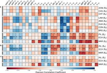
There are four distinct groups of glaciers with regard to the correlation of their glacier-wide mass-balances with potential predictors (Fig. 4). The first group consists of the Outer Tropics glaciers in Boliva (Zongo (ZON), Charquini Sur (CHS), Chacaltaya (CHT)) which are all significantly negatively correlated to summer 2 m air temperature (t) (α ≤ 0.05). The second group includes the subtropical glaciers of the Desert Andes (Los Amarillos (LAM), Amarillo (AMA), Guanaco (GUA), Conconta Norte (CON), Brown Superior (BRO)). These are characterised by high positive (~ 0.5 − 0.9) correlation coefficients for Ba and zonal wind speed at 850 hPa (u), and slightly lower, negative correlation coefficients for Ba and meridional wind speed at 850 hPa (v). The third group consists of the Central Andes glaciers PIL and ECH. Their annual mass-balances show significant positive correlation with precipitation (p) and u, and significant negative correlation with mean sea level pressure (slp), v, dew-point temperature depression at 850 hPa (dpd) and geopotential height at 700 hPa (h). The Ba of ECH is also significantly positively correlated with the Multivariate ENSO Index (mei), Antarctic Oscillation Index (aaoi) and u. The fourth group only consists of the glacier MAR, which is located in Tierra del Fuego. MAR's correlation pattern is similar to that of PIL and ECH. However, in contrast to PIL and ECH, there is a significant negative correlation with t, and a positive correlation with v. The remaining glaciers of the Desert Andes (AGN), Central Andes (AZF), Lakes District (Mocho Choshuenco SE (MCH)) and Patagonian Andes (ALC and De Los Tres (DLT)) did not yield significant results.

Fig. 4. Pearson correlation coefficients between the predictors (columns) and mass-balances of the glaciers (columns) of this study that meet the requirements for this analysis. Results are shown for (a) Outer Tropics (top), Desert Andes, Central Andes and Fuegian Andes (bottom) glacier annual mass-balance (Ba), (b) Central Andes (top) and Fuegian Andes (bottom) glacier winter mass-balance (Bw) and c) Central Andes (top) and Fuegian Andes (bottom) glacier summer mass-balance (Bs) separately. Seasonal mass-balances are only evaluated for the glaciers PIL, ECH and MAR due to lack of sufficiently long seasonal mass-balance records for the other glaciers. The predictors (Antarctic Oscillation Index (aaoi), Multivariate ENSO Index (mei), Pacific Decadal Oscillation Index (pdoi), 2 m air temperature (t), precipitation (p), mean sea level pressure (slp), zonal wind speed at 850 hPa (u), meridional wind speed at 850 hPa (v), dew-point temperature depression at 850 hPa (dpd) and geopotential height at 700 hPa (h)) are calculated for different months and seasons as described in section Predictor construction. Significance levels (from two-tailed tests) are denoted with asterisks in the figure (α ≤ 0.001: * **; α ≤ 0.01: * *; α ≤ 0.05: * ).
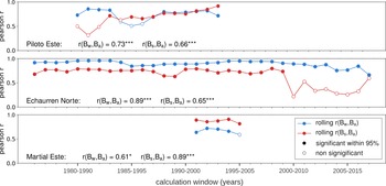
The winter mass-balances of PIL, ECH and MAR show a correlation pattern comparable to that of Ba. The main difference is the lack of a significant negative correlation with t for the glacier MAR. The summer mass-balance of PIL is not significantly correlated to any predictor variable. For ECH, the correlation with the respective predictors is generally weaker for Bs than for Bw. The Bs of MAR is significantly negatively correlated with t. Neither annual nor seasonal mass-balance of any glacier are significantly correlated with the pdoi. The correlation between seasonal mass-balances and Ba, computed from moving 10-year time windows for glaciers PIL, ECH and MAR, reveals a (mostly) stronger correlation of Bw with Ba for PIL, consistently stronger correlation of Bw with Ba for ECH, and a consistently stronger correlation of Bs with Ba for MAR (Fig. 5). For the glacier ECH, the correlation of seasonal mass-balances with Ba weakens from the calculation window 2000–2010 onward. The correlation coefficient values for Bs with Ba are more severaly reduced (from ~ 0.75 to ~ 0.4) and cease to be significant (Fig. 5).

Fig. 5. Correlations between winter mass-balance and annual mass-balance r(Bw,Ba) and summer mass-balance and annual mass-balance r(Bw,Ba) for the glaciers PIL (top), ECH (middle) and MAR (bottom). The plots show correlation coefficients calculated in 10-year moving windows. Filled dots indicate correlations that are significant (α ≤0.05) and empty dots indicate non-significant correlations. The correlation coefficients calculated over the total records are listed at the bottom of the plot for each glacier (α ≤ 0.001: * **; α ≤0.01: * *; α ≤0.05: * ).
3.2 Empirical glacier mass-balance models
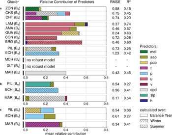
EGM performance varies significantly between glaciers. For Ba models, the RMSE ranges between 0.24 and 1.23 m w.e. with a mean of ~ 0.61 m w.e. The R 2 values lie between 0.15 and 0.74 and generate a mean of ~ 0.45. $r_{y\hat {y}}$ is significant (α ≤ 0.05) for all Ba models.
The four different groups identified by correlation analyses are also reflected in the estimated contribution to the total explained variance (R 2) by each predictor for each glacier (Fig. 6). Regional means of t and the El Niño-Southern Oscillation (ENSO) index are only chosen as robust Ba predictors for the Outer Tropics glaciers (ZON CHS and CHT) and contribute to the total explained variance with ~ 5 to ~ 15%. The annual mass-balance of the Desert Andes glaciers (LAM, AMA, GUA, BRO) is mostly explained by (u). This predictor is able to explain between ~ 35% (CON) and ~55% (BRO) of the predictand variance.

Fig. 6. Model skill measures (RMSE and R 2) and mean relative contribution of the different predictors (Antarctic Oscillation Index (aaoi), Multivariate ENSO Index (mei), Pacific Decadal Oscillation Index (pdoi), 2 m air temperature (t), precipitation (p), mean sea level pressure (slp), zonal wind speed at 850 hPa (u), meridional wind speed at 850 hPa (v), dew-point temperature depression at 850 hPa (dpd) and geopotential height at 700 hPa) to the total explained variance (R 2) for (a) the annual mass-balance of the Outer Tropics (top), Desert Andes, Central Andes, Lakes District, Patagonian Andes and Fuegian Andes (bottom) glaciers, (b) the winter mass-balance of the Central Andes (top) and Fuegian Andes (bottom) glaciers, and (c) the summer mass-balance of the Central Andes (top) and Fuegian Andes (bottom) glaciers. The RMSE and R 2 values are based on the final mass-balance regression models trained with ERA-Interim over the temporal overlap of ERA-Interim and available Ba record. The hatching of the bars represents the season over which the predictor is calculated. If the model selection algorithm fails to find a robust model, i.e. if no predictor passes the 40% threshold of being nonzero in the cross-validation loops, this is indicated in the figure.
The annual mass-balance variance of the glaciers of the Central Andes (PIL and ECH) and Tierra del Fuego (MAR) is mostly explained by regionally averaged anomalies of p and dpd.
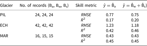
The RMSE values for the seasonal models of PIL, ECH, MAR are smaller than for the Ba models. The R 2 values for Bw and Bs models are similar and lower than those of the Ba models, respectively. The Bs model of glacier PIL shows no improvement over the prediction by the mean. The selected predictors of the seasonal mass-balance models are partly different from the predictors selected for the Ba models. The dominant predictors for Bw show the most overlap with the dominant predictors for Ba. There are only slight differences between Ba that is modelled directly and Ba that is constructed from its modelled Bs and Bw components. The three skill metrics are in the same ranges for the two differently modelled annual mass-balances and differ by ≤ ±10% for glaciers ECH and MAR and ≤ ±30% for glacier MAR. However, skill metrics values are generally slightly better (lower RMSE and higher R 2) for the mass-balance that is modelled from the seasonal mass-balances. An overview of the seasonal and annual performance metrics is provided in Table 3. The model performance metrics are higher for models trained over parts of the mass-balance records than for the models trained on the full mass-balance records if calculated from the training period. However, their prediction skills, as evaluated using completely independent data from the complementary half of mass-balance record, is significantly lower. Most of the models trained on these smaller data subsets have prediction skills with values of R 2 close to zero or even negative.
Table 3. Skill metrics (R 2 and RMSE) calculated from (1) observed Ba and directly modelled ${\hat {\rm B}}_{{\rm a}}$ (ŷ = ${\hat {\rm B}}_{{\rm a}}$
 ), and (2) observed Ba and modelled ${\hat {\rm B}}_{{\rm a}}$
 calculated from the modelled ${\hat {\rm B}}_{{\rm w}}$
 and ${\hat {\rm B}}_{{\rm s}}$
 components (ŷ =${\hat {\rm B}}_{{\rm w}}$
 + ${\hat {\rm B}}_{{\rm s}}$
 ) for the glaciers PIL, ECH and MAR
4. Discussion
4.1 Predictors of South American glacier mass-balance
Results of correlation analyses and predictor selection during EGM training give insights into the potential of different synoptic-scale climate variables as predictors for South American glacier mass-balance changes. Since considered predictors are chosen based on their physical relevance, our results may also highlight the relative importance of different atmospheric movements or processes for the studied glaciers. The computed correlation coefficients and predictor selection in EGM training reveal four distinct groups of glaciers. These comprise (1) Outer Tropics glaciers in Bolivia (ZON, CHS, CHT), (2) Desert Andes glaciers at ~ 29 °S (LAM, AMA, GUA, CON, BRO), (3) Central Andes glaciers at ~ 33°S (PIL, ECH) and (4) the glacier of Tierra del Fuego (MAR). This grouping is consistent with the findings of Sagredo and Lowell (Reference Sagredo and Lowell2012) and the glaciological zones proposed by Lliboutry (Reference Lliboutry1998), Barcaza and others (Reference Barcaza2017), and Zalazar and others (Reference Zalazar2020) (see also Fig. 1 and Table 1). Since no information about the glaciological zones was included in our analyses, our results provide independent evidence that confirm the merits of this classification for South American glaciers.
4.1.1 Outer tropics glaciers
Our findings identify summer 2 m air temperature (t), the Multivariate ENSO Index (mei) and summer dew-point temperature depression at 850 hPa (dpd) as decent predictors for Ba of Outer Tropics glaciers. This glaciological zone corresponds to group 2.2 cluster (Sagredo and Lowell, Reference Sagredo and Lowell2012), which is characterised by monthly temperature and precipitation means of ~ 0 to ~ 3 °C and ~ 0 to ~ 140 mm, respectively (Sagredo and Lowell, Reference Sagredo and Lowell2012). Generally, the outer tropical hydrological year can be divided into a dry season (austral winter) and a wet season (austral summer) (e.g. Francou and others, Reference Francou, Ribstein, Saravia and Tiriau1995; Sicart and others, Reference Sicart, Ribstein, Francou, Pouyaud and Condom2007), and both accumulation and ablation are highest in the wet season (e.g. Sicart and others, Reference Sicart, Ribstein, Francou, Pouyaud and Condom2007). This seasonal (summer) bias is reflected in our results. Previous studies identify the short and longwave radiation budget, which is closely linked to albedo, as an important determinant for Outer Tropics ablation (Rabatel and others, Reference Rabatel2013). Temperature integrates accumulation and ablation processes, as it is not only a measure of latent heat flux (long wave radiation budget), but also controls albedo (short wave radiation budget) by determining if precipitation falls as albedo-increasing solid (snow), thus adding mass to the glacier, or liquid (Rabatel and others, Reference Rabatel2013). It can thus be a predictor for mass-balance changes on the annual scale. Our identification of temperature as the most important predictor is therefore consistent with our knowledge of underlying mechanisms, especially given that the Outer Tropics glacier models are trained using Ba records. The onset of the wet season is important to Outer Tropics glacier mass-balance as highest melt rates occur at the end of the dry season when low values of glacier albedo and high values of solar irradiance prevail (Rabatel and others, Reference Rabatel2013). With the onset of the wet season, solar irradiance is reduced due to convective clouds, and albedo is increased by frequent snowfall. This special importance of seasonal distribution of precipitation may in parts explain the inclusion of summer dew point temperature as an important predictor in our models. Wagnon and others (Reference Wagnon, Ribstein, Francou and Sicart2001) show a time lag in the onset of the rain period during El Niño events, which results in negative mass-balance anomalies. This can explain the selection of mei as a robust predictor for the Ba of glacier CHS and the significant correlation mei to the annual mass-balance of glacier ZON.
4.1.2 Desert Andes glaciers
We identify zonal wind speed at 850 hPa (u), the Antarctic Oscillation Index (aaoi) and Pacific Decadal Oscillation Index (pdoi) as strong predictors for the mass-balance of our Desert Andes glaciers. These are located at high altitudes with mean annual temperature below 0 °C, which causes perennial solid precipitation (Rabatel and others, Reference Rabatel, Castebrunet, Favier, Nicholson and Kinnard2011). Monthly mean precipitation ranges from ~ 10 to ~ 50 mm (Sagredo and Lowell, Reference Sagredo and Lowell2012). Ablation mainly occurs via sublimation and only a small fraction of total ablation is achieved by melting (MacDonell and others, Reference MacDonell, Kinnard, Mölg, Nicholson and Abermann2013). Mass-balance variation are therefore predominantly controlled by changes in precipitation (Rabatel and others, Reference Rabatel, Castebrunet, Favier, Nicholson and Kinnard2011). Precipitation in these latitudes is primarily controlled by frontal activity in winter and convective storms in summer (MacDonell and others, Reference MacDonell, Kinnard, Mölg, Nicholson and Abermann2013). Since zonal wind speeds at 850 hPa are a measure of frontal activity, they are also related to precipitation variability. The choice of summer u as the main predictor for glaciers CON and BRO suggests the influence of the low-level jet. The two glaciers are located east of the other Desert Andes glacier (Fig. 1) in a region prone to summer snowfall events due to moisture transport by the low-level jet (Marengo and others, Reference Marengo, Soares, Saulo and Nicolini2004). This is consistent with the findings for the corresponding group of glaciers in Sagredo and Lowell (Reference Sagredo and Lowell2012). The influence of the Antarctic Oscillation (AAO) on LAM and AMA in our results can likely be explained by high latitude forcing for precipitation variability in northern-central Chile (Vuille and Milana, Reference Vuille and Milana2007) and the extent of regional impacts of the Southern Annular Mode (Gillett and others, Reference Gillett, Kell and Jones2006). The identification of the summer pdoi as a predictor for Desert Andes glaciers is supported by findings that precipitation anomalies in the same region are also associated with variations in Pacific Decadal Oscillation (PDO) (Quintana and Aceituno, Reference Quintana and Aceituno2012). However, we note that the true scale of the influence of the PDO cannot be estimated from the relatively short glaciological time series used in this study. In summary, the predictors we identified represent important controls on precipitation in these latitudes and are thus consistent with underlying mechanisms for ablation and accumulation.
4.1.3 Central Andes glaciers
In contrast to the glaciers of the Outer Tropics and the Desert Andes, the seasonality of the mass-balance year for the glaciers ECH and PIL (located at ~ 33 °S) is more accentuated (Pellicciotti and others, Reference Pellicciotti2008; Rabatel and others, Reference Rabatel, Castebrunet, Favier, Nicholson and Kinnard2011; Masiokas and others, Reference Masiokas2016; Ayala and others, Reference Ayala, Pellicciotti, Peleg and Burlando2017). More specifically, monthly temperature and precipitation means range from ~ −5 to ~ 5 °C and ~ 10 to ~ 160 mm, respectively (Sagredo and Lowell, Reference Sagredo and Lowell2012). Most of the total annual precipitation occurs in winters (Masiokas and others, Reference Masiokas2016) while the summers are very dry with often completely absent precipitation (Pellicciotti and others, Reference Pellicciotti2008). Our results suggest that PIL and ECH mass-balances are primarily controlled by regional precipitation or dew point temperature, which can serve as a proxy for precipitation. This is in agreement with the findings of Rabatel and others (Reference Rabatel, Castebrunet, Favier, Nicholson and Kinnard2011) and Masiokas and others (Reference Masiokas2016), who demonstrate that the mass-balance of ECH is driven by changes in precipitation, while temperature changes play a secondary role. The significant correlation with other predictors (aaoi, mei, slp, h) with Ba of ECH (and partly PIL) may be explained by their effects on precipitation variability. Since precipitation anomalies are controlling Ba, accumulation is found to be more important than ablation for ECH and PIL. This is additionally supported by weak correlations of the predictor variables with the Bs series of ECH and PIL and stronger correlations of the annual mass-balances with Bw than with Bs (see Fig. 5). The decoupling of ECH's Bs and Ba, and the weakening correlation of Bw with Ba from the calculation window 2000–2010 onward (Fig. 5) temporally coincides with the Central Chile Mega Drought (Garreaud and others, Reference Garreaud2019). Given that the primary control for ECH's mass-balance is precipitation, a prolonged drought can break down the otherwise strong empirical relationship. The glacier AZF does not have a sufficiently long mass-balance record to yield meaningful results.
4.1.4 Lakes District and Patagonian glaciers
We were unable to identify robust predictors for mass-balance of glaciers in the Lakes District (MCH) and more southern Patagonia (ALC and DLT). The glacier ALC had to be excluded from analysis entirely due to the absence of mass-balance records that temporally overlap with the reanalysis data. MCH and DLT likely still have too few measurements in succession (see Fig. 2) to produce meaningful results for the approach used in this study.
4.1.5 Fuegian Andes glaciers
The southernmost glacier MAR belongs to the group of glaciers in the Fuegian Andes, which experience monthly mean temperatures of ~ −1 °C in winter to ~ 5 °C in summer and precipitation rates of ~ 70 mm per month with low seasonal variation (Sagredo and Lowell, Reference Sagredo and Lowell2012). We identify dpd and summer t as the best predictors for mass-balance changes of MAR. Furthermore, precipitation anomalies correlate strongly with Bw and Ba. This is consistent with findings by Strelin and Iturraspe (Reference Strelin and Iturraspe2007), who attribute positive and negative mass-balance variations of the glacier MAR to humid-cool summer seasons and dry-warm years respectively. Precipitation anomalies are excluded from the mass-balance models of MAR in favour of the inclusion of dpd. This may be due to better representation of relevant precipitation variability by dpd at the location of the glacier.
4.2 Empirical glacier mass-balance models for South America
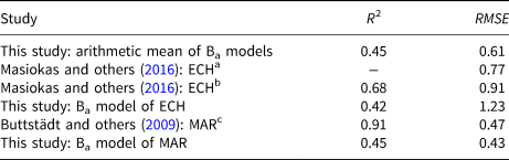
The Ba models of this study perform reasonably well with average performance metrics values RMSE ≈ 0.6 m w.e. and R 2 ≈ 0.5. We discuss these further in context of similar studies: Masiokas and others (Reference Masiokas2016) and Buttstädt and others (Reference Buttstädt, Möller, Iturraspe and Schneider2009) modelled net Ba in the same area thus allow a direct comparison to our results (Table 4). Schöner and Böhm (Reference Schöner and Böhm2007) and Mutz and others (Reference Mutz, Paeth and Winkler2015) adopted similar modelling techniques and thus provide a more suitable reference for evaluating the performance metrics values of our models.
Table 4. Comparison of skill measures (coefficient of determination (R 2) and root mean square error (RMSE)) of models from this study and models from Masiokas and others (Reference Masiokas2016) and Buttstädt and others (Reference Buttstädt, Möller, Iturraspe and Schneider2009)
a minimal mass-balance model.
b regression model.
c degree-day model.
Masiokas and others (Reference Masiokas2016) reconstructed the Ba for the glacier ECH based on a minimal glacier model (Marzeion and others, Reference Marzeion, Hofer, Jarosch, Kaser and Mölg2012) and two regression models using snowpack variations and local streamflow records as predictors. The minimal mass-balance model yields RMSE = 0.77 m w.e., whereas the regression models yield RMSE = 0.91 m w.e. and R 2 = 0.68. Buttstädt and others (Reference Buttstädt, Möller, Iturraspe and Schneider2009) employed a degree-day model to simulate the mass-balance evolution of MAR from 1960 until 2099. In the calibration period, their model yields R 2 = 0.91 and RMSE of 0.47 m w.e. Where comparisons are possible, the models of this study do not perform as well as previous models of Masiokas and others (Reference Masiokas2016) and Buttstädt and others (Reference Buttstädt, Möller, Iturraspe and Schneider2009) (Table 4). This is expected, since our models use synoptic-scale atmospheric predictors, while the other studies either use a completely different approach, i.e. minimal mass-balance model and degree-day model, or incorporate local (proxy) data like streamflow and snowdepth records, which may hold further important information. Additionally, Buttstädt and others (Reference Buttstädt, Möller, Iturraspe and Schneider2009) do not apply any cross-validation to their degree-day factor calibration. This likely leads to a higher skill in the training period, but also increases the risk of overfitting.
Some of our models can compete with the RMSE and R 2 values of similarly constructed mass-balance models for glaciers in Austria (Schöner and Böhm, Reference Schöner and Böhm2007) and Norway (Mutz and others, Reference Mutz, Paeth and Winkler2015). Even though the climatic settings are different, the comparison shows that the performance scores for a subset of our glacier models are within the published range for EGMs of this type. The overall better performance by the models of previous studies can likely be attributed to the availability of more complete datasets and longer measurement records. These increase the probability of adequately capturing the relationships between synoptic-scale atmospheric variability and mass-balance changes during model training. Furthermore, they allow separate modelling of summer and winter mass-balances, which may result in better predictions of Ba (Schöner and Böhm, Reference Schöner and Böhm2007). Overall, our results are satisfactory and speak in favour of adopting an empirical mass-balance modelling approach in South America to complement physical-numerical models.
4.3 Limitations and suggestions
The main shortcomings of our models can be summarised as (i) a frequent underestimation of the amplitude of predicted mass-balance variability, (ii) low performance scores for some models, (iii) uncertainties arising from mostly modelling Ba directly instead of constructing it from modelled seasonal components Bw and Bs, and (iv) the neglect of glacier dynamics that are important for predicting the long-term response to climate change. We can subdivide the limitations into the categories of data sparsity and quality, and methodological limitations.
4.3.1 Data sparsity and quality
A significant problem for the approach of this study is the still very limited data base for glaciers in South America. Although we adopted methods to prevent overfitting and increase the models’ robustness, the predictive capabilities of EGMs remain more uncertain when mass-balance records are not sufficiently long enough to subdivide it into completely independent training and validation period. Furthermore, the required length of the data records depends on the frequency of climatic events that affect the glacier. Therefore, the short records are particularly problematic for outer tropical glaciers, which are more directly influenced by lower frequency ENSO cycles. Pooling the data records for glaciers of the same regime and constructing more general models for a cluster of glaciers may be an option to circumvent this problem.
Due to limited glacier data records, only Ba models can currently be constructed for most of the glaciers studied here. This leads to a bias in the selection of predictor towards climatic factors in the season that is the stronger determinant of Ba. A change in the glaciological regime that leads to a shift from ablation-controlled to predominantly accumulation-controlled Ba (or vice versa) will compromise the accuracy of the EGMs. Our results indicate that this may be a problem for the Ba EGM constructed for PIL and ECH (Fig. 5).
Glaciological mass-balance records are heavily biased towards small glaciers, while most of the ice in the Andes is stored in larger glaciers. The same is true for the glaciers of this study (see Area in Table 1). Furthermore, our study is unable to produce meaningful results for any of the glaciers in the Lakes District and Patagonian Andes, which contribute ~95% to the total ice volume in the major glacier regions of southern South America (Carrivick and others, Reference Carrivick, Davies, James, Quincey and Glasser2016). The reader is advised to consider these representation issues.
The quality of relevant data is compromised by both logistical and technological factors. For example, the often difficult access to glaciers can result in delays for in-situ measurements that can ultimately lead to underestimations of winter accumulation (or summer ablation). These constitutes additional sources of uncertainty for predictions generated by EGMs.
The lack of relevant atmospheric variables in available datasets is another problem. For example, there are factors such as atmospheric black carbon from human emissions and wildfires, which can have an influence on the mass-balance of Andean glaciers (Molina and others, Reference Molina2015; Magalhães and Evangelista, Reference Magalhães and Evangelista2018), but cannot be considered here, because the ERA-Interim reanalysis data contain no measure for such atmospheric aerosol content.
4.3.2 Methodological limitations
The strength of our approach is given by the focus on synoptic-scale controls, its cost-effectiveness, and the possibility to directly couple of the EGMs to general circulation models (GCMs). However, the EGMs should be regarded as models that complement rather than replace others, such the Open Global Glacier Model (OGGM) (Maussion and others, Reference Maussion2019), as they come with several notable drawbacks:
1. Predictor multicollinearity: The general underestimation of the amplitude of predicted mass-balance indicates a tendency of underfitting. The measures adopted to mitigate the problems of multicollinearity among predictors and avoid overfitting may encourage the models to generalise to a greater extent than necessary. The same measures may also create competition among predictors in the cross-validation setting to make it into the final model. In some cases, this can lead to the exclusion of important predictors (Mutz and others, Reference Mutz, Paeth and Winkler2015). The introduction of least absolute shrinkage and selection operator (LASSO) variable selection and regularisation may improve the EGMs. It is known to deal well with multicollinearity (Tibshirani, Reference Tibshirani1996) and has been successfully used for statistical climate downscaling (Hammami and others, Reference Hammami, Lee, Ouarda and Lee2012; Gao and others, Reference Gao, Schulz and Bernhardt2014) and also in a glaciological context (Maussion and others, Reference Maussion, Gurgiser, Großhauser, Kaser and Marzeion2015). Another way to prevent problems related to multicollinearity is through the construction of new, uncorrelated predictors. This may be achieved by conducting a principal component analysis (PCA) on the set of predictor variables used in this study (see Table 2).
2. Predictor representation: It is likely that the predictors of this study do not adequately capture all important synoptic-scale atmospheric variability. This is a problem especially for low-frequency changes that are not observed in the short time covered by the mass-balance records. Possible improvements include an optimisation of the radius used in the construction of spatial means, or the fine-tuning of predictors, such as the choice of different pressure level dew-point temperature for studies with a more regional focus.
3. Assumption of linearity: Our approach uses parametric statistical models that assumes a linear relationship of glacier mass-balance and the large-scale state of the atmosphere. Problems arising from this approach may be bypassed, for example, by using a different family of regression procedures for the transfer functions, such as Random Forests (Breiman, Reference Breiman2001). Bolibar and others (Reference Bolibar2020) demonstrate that a deep-learning approach is able to capture non-linear behaviour that is missed by classic regression-based techniques.
4. Temporal stationarity of transfer functions: Our approach assumes that the models’ transfer functions are stationary in time. It does not take into consideration factors and mesoscale processes that likely affect mountain glaciers (Mölg and Kaser, Reference Mölg and Kaser2011) and potentially lead to temporal instability of the transfer functions. These factors also include changes in albedo, which is important for the energy balance on the glacier and thus affects ablation. Regional mean albedo changes can be caused by different ablation zone extents if the equilibrium line altitude increases (Sagredo and others, Reference Sagredo, Rupper and Lowell2014) or glaciers shrink (Gurgiser and others, Reference Gurgiser, Marzeion, Ortner and Kaser2014). Another factor are local katabatic winds that may affect ablation processes. This has been shown for the tongue of the Juncal Norte glacier (Pellicciotti and others, Reference Pellicciotti2008), which is located in the same area as the glaciers ECH and PIL. For a more general discussion of spatio-temporal transferability of glacier mass-balance models, the reader is referred to Zolles and others (Reference Zolles, Maussion, Galos, Gurgiser and Nicholson2019).
5. Topography and glacier dynamics: A major limitation of our models is the neglect of ice dynamics and geometry, and the implicit assumption of constant topography and glacier altitude during model training. The models are thus unable to produce the dynamic response to climate-glacier imbalances (Zekollari and others, Reference Zekollari, Huss and Farinotti2020) that would change the timing and magnitude of glacier mass changes. This has serious implications for the application potential of the EGMs presented in this study. The models’ transfer functions are specific to the altitude (range) of the glaciers during model training. They capture the synoptic scale climatic drivers of MB of each glacier in their topographic setting of the recent past and present-day. When altitude changes more significantly as the glacier responds to larger climate-glacier imbalances, the transfer functions of the model can no longer be regarded as valid. Therefore, the application of the EGMs presented here is only merited for predicting the short-term glacier response to changes in climate. The dynamic response may be approximated in a limited way by pooling the mass-balance data for glaciers at different altitudes in a similar glaciological zone, training altitude-specific models and implementing dynamic model selection controlled by predicted shifts in altitude. As mass-balance records continue to grow, the inclusion of topographic predictors in a deep-learning approach (e.g. Bolibar and others, Reference Bolibar2020) represents another promising way to address this limitation.
Table 2. Overview of all climate predictors and their acronyms used in this study
5. Conclusion
We assessed the control of synoptic-scale atmospheric factors on the mass-balance of 13 glaciers in South America by means of correlation analyses. The predictive capabilities of the same factors were evaluated in the training procedures for the EGMs of each glacier. The training procedure consisted of a cross-validated stepwise multiple regression with forward selection and robustness filter for predictors. The key findings of this study are the following:
• The assessment of synoptic-scale climatic controls on South American glaciers reveal four distinct groups. The glaciers of a specific group are in geographical proximity and characterised by similar sets of important synoptic-scale predictors. The four groups can be summarised as follows: (1) The mass-balance variability of Outer Tropics glaciers in Bolivia is linked to 2 m air temperature (t) and the El Niño-Southern Oscillation, (2) the glaciers of the Desert Andes are primarily influenced by zonal wind speed at 850 hPa and the Antarctic Oscillation (AAO), (3) the glaciers of the Central Andes are mainly controlled by precipitation anomalies, dew-point temperature depression at 850 hPa (dpd) and the AAO, and (4) the mass-balance of the glacier Martial Este in the Fuegian Andes is linked to dpd and summer t.
• The four distinct groups (above) are coincident with previously proposed classifications of South American glaciers. Our results therefore support the merits of the subdivision into the glaciological zones proposed by Lliboutry (Reference Lliboutry1998) and updated by Barcaza and others (Reference Barcaza2017), and Zalazar and others (Reference Zalazar2020).
• The annual mass-balance EGMs have an average R 2 value of ~ 0.45 (0.15–0.74), and an average RMSE value of ~ 0.61 m w.e (0.24–1.23 m w.e). The Outer Tropics EGMs perform worst (R 2 ≈ 0.3) and Desert Andes EGMs perform best (R 2 ≈ 0.6).
• The EGMs do not consider glacier dynamics or geometry, which are important factors for predicting the long-term mass-balance response to climate change. Therefore, they are currently only suitable for predicting short-term responses to perturbations in climate.
• The empirical relationship between Echaurren Norte's Bs and Ba breaks down from the 2000–2010 onward. This is likely related to the Central Chile Mega Drought.
The reader is advised to carefully consider the listed limitation and suggestions before applying this study's approach or results. While our results speak in favour of an EGM-based approach to glacier mass-balance modelling in South America, we suggest several measures to increase the accuracy and reliability of the models. A cross-validated LASSO approach may improve the EGMs, as its way to deal with multicollinearity may result in fewer problems than the approach used in this study. Furthermore, the glacier groups identified in this study may allow the pooling of data and the construction of more general, group-specific EGMs to circumvent the problem of the short mass-balance records. Another way to address this problem is by incorporating geodetic mass-balance records, and to use these to constrain mass-balance changes over specific observational periods and glaciological zones. Potential glacier regime shifts, i.e. non-stationary glacier-climate relationships, could also be addressed by a Bayesian model selection approach provided that observational records are long enough to allow the construction of regime-specific EGMs. Further improvement of the EGMs may be possible by considering topographic predictors in a deep-learning approach that would be able to capture important non-linear behaviour. Finally, we suggest the coupling of improved EGMs to a multi-model GCM ensemble to assess the effects of inter-model differences on mass-balance predictions.
Supplementary material
The supplementary material for this article can be found at https://doi.org/10.1017/jog.2022.6.
Acknowledgements
Support for this project was provided by DFG grant EH329/14-2 to T. Ehlers. We thank the European Centre for Medium Range Weather Forecasts for providing the ERA-Interim reanalysis data, and thank the World Glacier Monitoring Service (WGMS) for providing the glacier data used in this study. We also thank the World Climate Research Programme and the climate modelling groups, the Max Planck Institute for Meteorology, for producing and providing their model output. Finally, we thank the scientific editor Fanny Brun and the two anonymous reviewers for their very thorough and helpful reviews of our manuscript.


 Open access