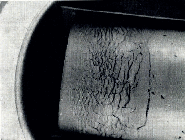
If the temperature of the surface of moist ground is suddenly lowered below the freezing point of water, as in a sudden frost, then it often happens that the soil does not freeze homogeneously but that instead there form lenses of almost pure ice, separated by unfrozen soil. These lenses may be from less than 1 mm. to several centimetres thick, they are roughly parallel to the surface and the distance between consecutive lenses increases with increasing depth. This phenomenon has been described by Reference TaberTaber (1929, Reference Taber1930), Reference BeskowBeskow ([1935]), Reference HigashiHigashi (1958) and others. A photograph of lenses produced in the laboratory is given in Figure 1. As a result of ice segregation, the surface of the soil lifts or “heaves”. Frost heave has attracted the attention of many investigators but only Reference MartinMartin (1958) has discussed why several ice lenses form instead of the one which forms first continuing to grow indefinitely.
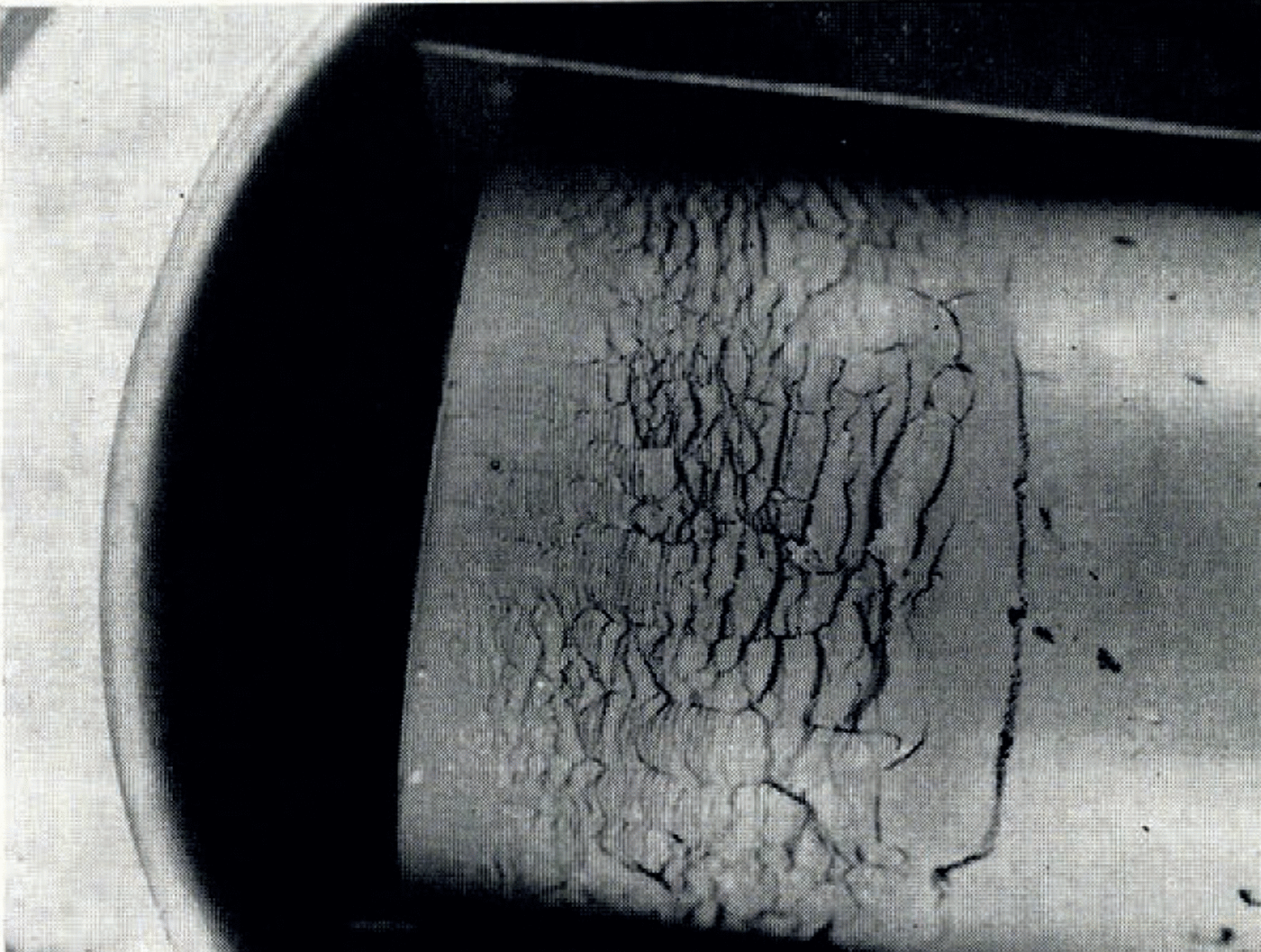
Fig. 1. Ice lensing in frozen clay
In this paper it is shown that a simpler theory than Martin’s is sufficient to explain the formation of separate lenses, and a mathematical development of the problem suggests when they might be expected to appear. The aim is not to give the most general description of the soil system but rather to study the simplest model which still exhibits ice Iensing.
An analogy between ice lenses and Liesegang rings was first suggested by Reference Shemyakin and MikhalevShemyakin and Mikhalev (1938). Liesegang rings, called after their discoverer, are periodic precipitates produced in a chemical system when two interdiffusing substances react to form an insoluble product. Liesegang placed a drop of silver nitrate solution on the surface of a gelatin layer containing potassium dichromate. The two reacted to form red silver chromate but he observed that the precipitate did not spread out continuously from the original drop. Instead concentric red rings were formed, the space between them remaining clear. A theoretical explanation depends on the necessity of supersaturation before precipitation can begin. As precipitation occurs at the original drop, silver ions diffuse outward, but precipitation does not occur immediately outside the original zone because the concentration of chromate ions there has been reduced by their diffusion inward. For a new precipitate to be nucleated the ionic product of the silver and chromate ion concentrations must reach a certain supersaturation product, and this happens first at some distance beyond the original precipitation zone. The process then repeats itself.
Reference Shemyakin and MikhalevShemyakin and Mikhalev (1938) showed that the distances between consecutive ice lenses in Taber’s published photographs of frozen soils satisfied a semi-empirical relationship between the spacings of Liesegang rings developed by Reference JablczynskiJablczynski (1926). On this basis they concluded that ice lensing and Liesegang ring formation were “absolutely analogous”. Reference MartinMartin (1958) considered a semi-infinite mass of homogeneous saturated soil at a uniform temperature above freezing, and he supposed that the surface was then suddenly brought into contact with a large mass of ice at a temperature below freezing. Immediately more ice begins to form at the interface and water flows from the soil to the freezing front; so that this shall happen there must be a pore-water pressure gradient in the soil, and at the freezing front the water pressure is reduced.Footnote * Martin then asserted that, as time goes on, the surface ice will grow more and more rapidly, while the ability of the soil to supply water will diminish, and therefore the temperature at the freezing front will fall. This fall in temperature will further increase the “demand” for water by the ice but still further reduce the rate of water supply, because the increased suction in the pore water is accompanied by an increasing compressive stress in the soil and a correspondingly reduced permeability. This process will “snow-ball” and the rate of ice formation fall, and now a freezing temperature will spread into the unfrozen soil beyond the ice front. Ice cannot form there immediately because no ice nuclei are present, and will only do so when the temperature falls to a nucleation temperature below the equilibrium freezing point. Ahead of the ice front, the ice-nucleation temperature is reduced by the fall of the equilibrium freezing point following on the fall in pore-water pressure (which corresponds to the reduced number of chromate ions beyond the original precipitate in the Liesegang ring analogue). However, the nucleation temperature falls more slowly than the temperature itself, and eventually the temperature falls below the nucleation point at some point within the soil and a new ice lens is nucleated there.
Although an ice crystal nucleated in supercooled water will certainly grow very rapidly at first, it is not clear why its growth rate should increase with time—as is suggested in Martin’s argument—and indeed theoretical studies of ice crystal growth (Reference MasonMason, 1957) suggest the opposite conclusion. One would expect that as time went on the temperature and water-content gradients close to the nucleated lens would fall, this would reduce the heat flow from and water flow to the lens, and that the growth rate would decrease. This conclusion is supported by the following theory.
Heat and Water Transport in Freezing Soil
A mathematical model of the diffusion processes in the soil will be considered first. Reference GlobusGlobus (1962) has shown that for saturated soils at large water contents the effect of thermal diffusion on water transport is negligible compared with that of soil moisture potentials set up by ice formation. Water diffusion is therefore governed by the one-dimensional diffusion equation
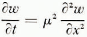
where ω is water content (referred to unit mass of dry soil), x is distance, t is time and μ 2 is the diffusion coefficient. The rate at which water crosses unit area perpendicular to x is κμ 2 ∂ω/∂x where κ is a numerical factor to allow for ω being referred to unit mass of dry soil instead of unit volume of wet soil. The temperature field is governed by
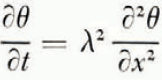
where θ is temperature and λ 2 is thermal diffusivity; it can be shown that the omission of a term in this equation expressing the effect of heat convected by flowing water has a negligible effect. It is known from experiment (Reference NersesovaNersesova, 1950; Reference WilliamsWilliams, 1964) that water in soil reaches equilibrium with ice at a lower temperature than does free water. This temperature will be denoted θ F ; it is a function of the water content of the soil, and this function can be determined by direct experiment and through the thermodynamics of soil moisture (Reference CroneyCroney and others, 1952). If ice is forming at a point within the soil or at its surface, the temperature there must be θ F ,Footnote * that is, if ice is forming at x at time t
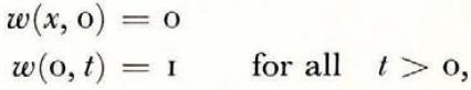
Consider first a very simple situation closely similar to that studied by Reference MartinMartin (1958). A semi-infinite mass of uniform saturated soil occupying the region x > 0 is initially at a temperature θ 0 and water content ω 0. The initial temperature is such that θ 0 = θ F (ω 0). At time t = 0 the temperature of the surface is suddenly lowered to θ 2 which is sufficiently low for ice to nucleate immediately. Ice then forms at the surface of the soil and grows into the region x < 0; the temperature at the surface of the ice is held at θ 2. The thickness of the ice is y(t). Initial and boundary conditions for the diffusion problem are thus
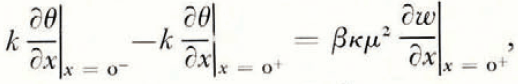
At the soil/ice interface the soil is in local equilibrium with ice, and also a heat balance and a mass balance can be written. If we assume for simplicity that the thermal conductivities of soil and ice are equal, and denote them by k, and let ρ i be the density of ice, ρ w the density of water, and β the latent heat of freezing of unit volume of water,

A solution for the temperature and water-content fields presents no difficulty. Since there is no characteristic length, the diffusion equations (1) and (2), and the balance conditions (8) to (10) can be transformed into a set of ordinary differential equations with independent variable


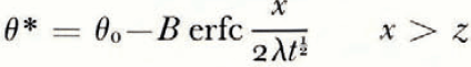
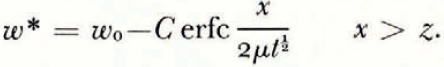
where θ(0, t) can be uniquely determined from the balance conditions. If θ F is a linear function of ω over the range ω 0 to ω(0, t), then
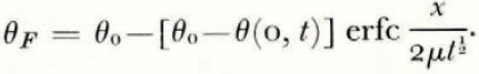
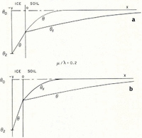
If μ > λ, the space distributions of θ and θ F at a time t are as illustrated in Figure 2a.
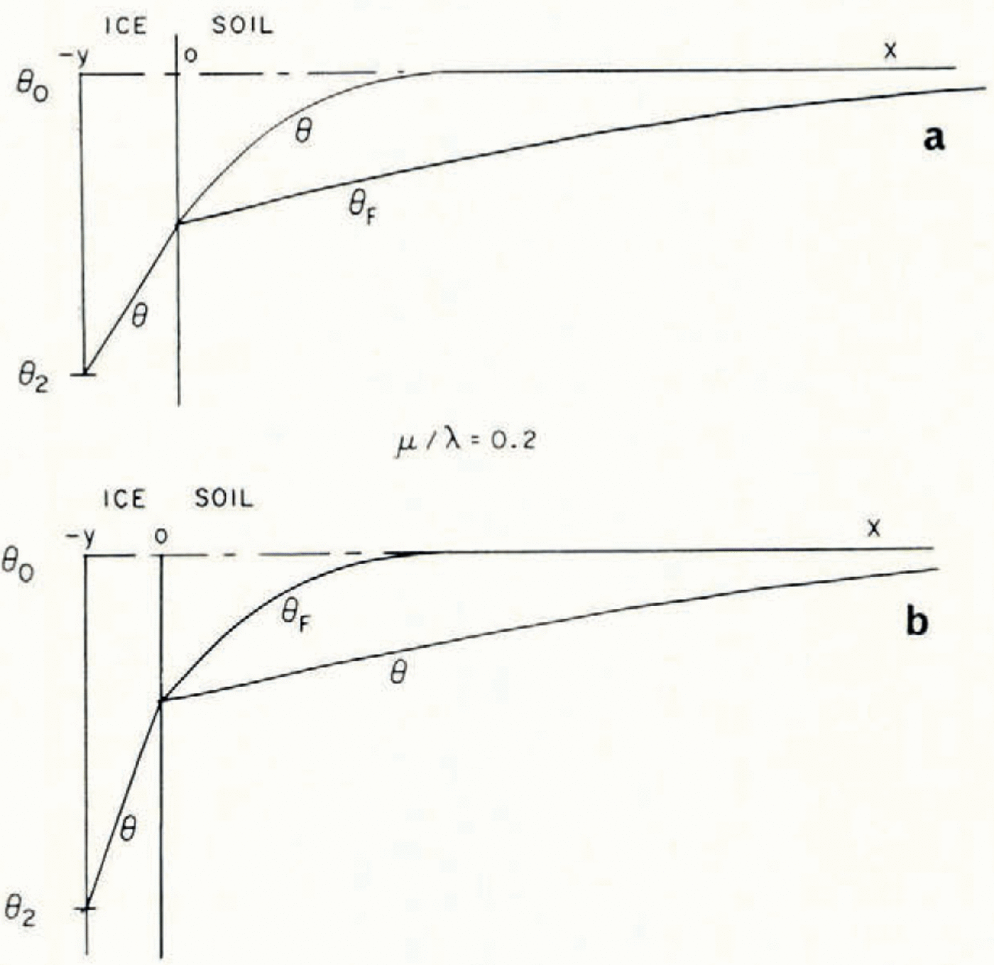
Fig. 2. Temperature and θ F distributions in simple models of a soil freezing system
Everywhere in the soil θ > θ F , that is, the temperature is greater than the temperature at which the soil at its existing water content would be in equilibrium with ice, and therefore there is no possibility of nucleation of a new ice lens. If, on the other hand, μ < λ, then the distributions are as illustrated in Figure 2b; θ < θ F in x > 0, and there is a possibility of the nucleation of a new lens ahead of the first freezing front. Denote the difference θ F – θ by θ n; only if θ n is positive is nucleation possible. It is a measure of supercooling, and the greater θ n is, the more likely is nucleation to occur. For all t > 0, the position where lens nucleation is most likely is beyond the original ice/soil interface.
Even the heterogeneous nucleation of ice in water or water vapour is not a well-understood process, though it has been far more studied than ice nucleation in soil. We can, however, expect that the qualitative pattern of behaviour will be similar. Ice particles are nucleated at a rate which increases very rapidly with increasing supercooling, but at a fixed temperature it is constant with time. If the temperature and ω fields are as this simple model suggests, the first nucleation of a lens will be less likely to occur at a point very close to x = 0 than farther away. Close to x = 0, θ n will rise rapidly but only remain near the maximum value for a very short time before falling towards zero; farther away θ n will rise less rapidly but remain close to the maximum longer. It follows that even this severely idealized model of the diffusion and nucleation processes in freezing soil does predict the formation of distinct ice lenses and that, although the far more complex processes of Martin’s model may occur, they do not seem necessary for lens nucleation.
In general μ/λ is about 0.1 for silt and silty clay, about 0.4 for colloidal clay and about too for sands. It has been observed (Reference Linnell and KaplarLinnell and Kaplar, 1959) experimentally and in the field that silty clays are most susceptible to frost heave, fine-grained “fat” clays rather less so and that multiple ice lensing does not occur at all in sands and gravels (although a single ice lens can form and grow even in these). This lends some support to the present theory.
What happens after a new ice lens is nucleated ? In all that follows, x at the nth ice lens within the soil will he denoted x n and the time at which that lens nucleates by t n .Footnote *Immediately after t 1 the temperature at x 1 rises rapidly to a temperature just below θ F (x 1, t 1 −) but well above θ(x 1, t 1 −); this rise in temperature is produced by the latent heat evolved in freezing and it is parallel to the sudden rise in temperature of a supercooled free liquid when freezing begins. The temperature must remain a little below θ F (x 1, t 1 −) because, if the originally infinitesimal ice nucleus is to grow, water must flow towards it and so there must be a water concentration gradient in the surrounding soil. Since the temperature at x 1 rises, the temperature at points near to x 1 (on either side) will later rise too, as the temperature change diffuses outward. Farther away the effect is less pronounced and there the temperature will not rise, but its rate of fall will be checked. Since μ < λ, temperature changes diffuse faster than water-content changes, and so the temperature gradient at x = 0 will increase before the water supply to x = 0 (where freezing is still going on) is affected. Then the net heat flow from x>0 is insufficient to freeze all the water arriving from x>0 and so the temperature at x = 0 will also rise. Later, however, the change in water content at x, will affect the concentration gradient at x = 0, and the flow of water from the space between the lenses to both x = 0 and x 1 will be reduced. This in turn will induce a fall in temperature both at o and x 1. The rate of freezing will fall slowly at x = 0, which can only draw water from x < x 1 and finally the rate of ice formation at o will have almost vanished, ice at x, will be forming almost exclusively from water from x > x 1, and the temperature at x 1 will be close to θ(0, t < t 1). Then the θ and ω distributions will be qualitatively similar to those at t 1 −, although mathematically much more complex, and the process will repeat itself.
Ideally, we should like to be able to determine the temperature of water-content distribution in systems like that illustrated in Figure 1. Nucleation, however, is a process obeying statistical laws. Even when lens nucleation in soil is more fully understood, it will only be possible to speak of the probability that a lens will be nucleated within a certain time at a certain temperature. This, and the complexity of the equations, means that it will be impossible to follow in detail the development of the successively more complicated θ and ω fields as more and more lenses form. In experiments we find that, except immediately after the beginning of freezing, the number of ice lenses is large and the distance between them small compared with the distance from the original freezing front to the farthest ice lens. If we can find the “smoothed-out” temperature and water-content fields which would develop if the freezing front moved into the soil smoothly instead of in discontinuous jumps from x n to x n+1, then we can expect this field to coincide with the real fields except within distances from the freezing front of the same order as the distances between lenses. This smoothed-out solution will be represented by θ * (x, t) and ω * (x, t)
Here we consider a slightly less severely idealized model of a semi-infinite mass of homogeneous saturated soil whose surface temperature is suddenly lowered. The initial temperature is θ 0, the initial water content is ω 0 and the initial equilibrium freezing temperature of the soil, θ F (ω 0), is equal to θ 1. The solution only applies at times large compared with t 1, and therefore the thickness of the surface ice is negligible and the boundary condition becomes
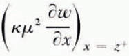
The thickness of the frozen layer is z(t), from x = 0 to the continuously advancing freezing front of this smoothed solution. Then temperature diffusion is governed by Equation (2) in the region (0, ∞) and the water-content distribution by Equation (1) in (z, ∞), the unfrozen region. At the freezing front x = z and the heat balance is
where γ is the appropriate latent heat of freezing of unit volume of the soil and the other quantities are as defined earlier. It is assumed that once the freezing front has passed a point in the soil no further water diffusion takes place there. In other words, there is no water diffusion in x < z, and in particular no contribution to Equation (15) from water diffusing to the freezing front from unfrozen water on the cold side. Immediately on the cold side of the last ice lens to form, the soil between lenses is in equilibrium with ice at the temperature of the lens, but equally, immediately on the warm side of the same lens soil is in equilibrium with ice at the same temperature (if we neglect the very small temperature difference across a lens). Therefore, there is no change in the unfrozen water content of the soil as the freezing front passes through it, and γ can be set equal to zero; the only latent-heat contribution to condition (4) is βκμ 2 ∂ω */∂x, the heat evolved in the formation of lenses.
However, the θ * and ω * fields are not uniquely determined by these initial and boundary conditions. If, to take the simplest case, μ and λ are constants, then the initial conditions, the boundary conditions and the diffusion equations are satisfied by
There is no characteristic length and
-
i. Nucleation ahead of the freezing front is impossible. Then the ice lens which forms first continues to grow indefinitely, z remains zero and the solution is similar to that for the simpler model considered earlier.
-
ii. There is no barrier to ice nucleation in x > 0. Ice forms as soon as the temperature falls to θ 1 without any supercooling or freezing-point depression. Then ice formation takes place at θ 1 = θ F [ω 0], no water-concentration gradient is set up in the soil, there is no movement of’ water and we have the in situ freezing problem of classical heat conduction theory, the Stefan problem (Reference Carslaw and JaegerCarslaw and Jaeger, 1959).
Both extreme cases can be observed in nature but neither corresponds to the formation of multiple lenses. If lensing takes place, the freezing front advances at a rate less than that given by the Stefan problem solution.
It follows that the rate at which the freezing front advances depends on the details of the ice-nucleation process, which are still obscure. If, however, the rate of freezing-front advance is known, then the temperature and water-content fields throughout the system can be found; this can be done numerically even if the diffusivities are not constant. In a later section a solution for a varying water-diffusion coefficient is found. Once the water-content field is known, the rate at which water crosses the freezing front follows. In a small time interval dt the volume of soil which becomes part of the frozen region is (dz/dt)dt and this soil has a water content equal to that immediately on the warm side of the freezing front; at the same time a volume of water
This computation only gives the smoothed θ * and ω * fields. Nucleation of new ice lenses depends not on the smoothed fields but on the perturbation close to the freezing front which results from the advance of the freezing front in discrete jumps from x n to x n+1. If n is large, we can expect that the freezing process is periodic in the sense that the temperature and water distributions at t n+1 − (immediately before lens n+1 is nucleated) are identical to the distributions at t n − (immediately before lens n is nucleated) shifted through a distance x n+1−x n in the positive x direction. That is
It is possible to express this evolution in the interval (t n , t n+1) through two integral equations for the unknown functions θ(x, t n −) and ω(x, t n −). The functions are subject to additional conditions expressing heat balances at x n and x n+1, the condition that at those points θ(x, t) = θ F [ω(x, t)], and the condition that θ → θ * and ω → ω * as x → ∞. Unfortunately these integral equations have proved intractable.
An approximate “order of magnitude” estimate of the relation between x n+1−x n and t n+1−t n for n large is given by the following argument. If μ is small compared with λ, water-content changes diffuse much more slowly than temperature changes. The position of a new ice lens depends on the position of a maximum in θ n = θ F − θ. Since θ F changes depend on water content, the position of the maximum will depend primarily on water diffusion, if that is much slower than temperature diffusion (cf. Fig. 2b). Although there is of course no finite propagation velocity associated with water diffusion, there is a relation between the magnitude of a response, the distance from its stimulus, and the time. If

then
If the effect at (x, t) is neither small compared with the disturbance at (0,0) nor almost as large as the disturbance,

If an ice lens is nucleated at x n , θ and θ F at (x n , t n +) are close to θ F (x n , t n −); this temperature will not begin to drop at xn until the rate of ice formation at x n−1 is restricted by the ice lens at xn . We can distinguish four stages in the chain of events between tn and t n+1:
If the speed of the process is determined by stages (ii) and (iv), a water-content change “travels” 2(x n+1−x n ) in (t n+1−t n ), from xn to x n−1 (stage (ii)) and from xn to x n+1 (stage (iv)). Therefore, it seems likely that

Description of Experiments
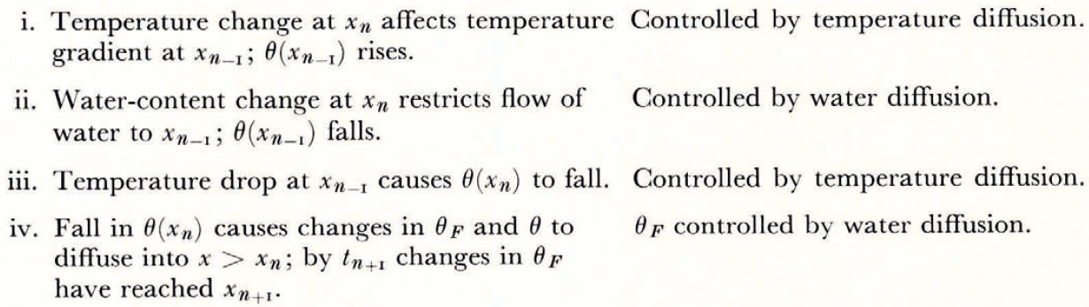
A number of experiments were carried out to investigate ice-lens formation and to compare observations with the predictions—some qualitative, others quantitative—of this model. The apparatus used is illustrated schematically in Figure 3. A cylinder containing moist clay, initially at room temperature, insulated on its sides and at one end, is placed in contact with a brass plate whose temperature is controlled. The cylinder is sufficiently long that in the duration of each experiment there is no alteration of water content at the end remote from the cooled end; it therefore behaves as would a semi-infinite cylinder. The temperatures at different points on the cylinder axis are measured by thermocouples. At the end of the experiment the soil can be removed from the cylinder, photographed and then dissected so that the water content can be determined by weighing sections before and after drying.
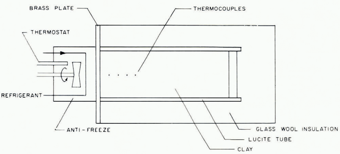
Fig. 3. Schematic diagram of experimental apparatus
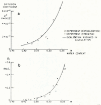
The soil used in the investigation was re-moulded Boston blue clay; its measured grain-size distribution is given in Table I. The relation between ω and θF was determined indirectly from consolidation experiments to determine the moisture potential,Footnote * and it was checked against direct measurements. In small changes in water content, the relation between moisture potential and ω can be linearized, and then the water-diffusion coefficient μ 2 is identical to the “coefficient of consolidation” of the linearized engineering theory of one-dimensional consolidation. A one-dimensional consolidation test, then, in which loads were applied in increments which produced decreases in water content of the order of 0.025, served both to determine the θ F , ω relation and to find μ 2 at different water contents. In Figure 4 are given the experimental relations between θ F and ω, and μ 2 and ω.Footnote †
Table I Clay Particle-Size Distribution (By Sedimentation)

Fig. 4. Diffusion coefficient μ2 and equilibrium freezing temperature θF as functions of water content (Boston blue clay)
Figure 1 illustrates the type of ice lensing observed in these tests. The cylinder containing clay at room temperature and uniform water content was brought suddenly into contact with the pre-cooled brass plate and then held there for the remainder of the test. Owing to the initial rapid heat flow to the plate, the plate temperature would rise several degrees at first, but it quickly returned to its original value. Tests lasted several hours and so the real temperature change closely approximated a “step-function” decrease at the end of the cylinder.
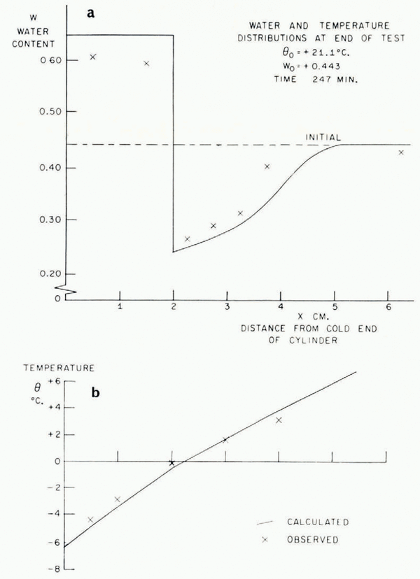
In Figure 5 the temperature/time relationships at different points in the soil in a typical test are described. The most striking features are the arrests in the temperature/time curves which occur shortly before and after the temperature reaches 0°C. This is exactly what the present theory predicts, that the sudden rise in temperature at the point where a lens is nucleating should produce increases in temperature at points nearby and retard cooling farther away. In Figure 6 are illustrated the temperature distribution at the conclusion of a test and the simultaneous water-content distribution. As this theory predicts, ahead of the freezing front the water content is reduced and in the frozen zone it is very much increased. Temperature and water-content distributions for a second test are given in Figure 7b, together with a photograph of the soil cylinder immediately before dissection (Fig. 7a).Footnote * The scar about 1 cm. from the freezing front is a surface phenomenon which occurred in several tests and it is probably associated with the severe shrinkage stresses developed in the unfrozen region. This effect has been neglected in the idealized model of the diffusion process developed here, in which it has been assumed that water diffusion is governed only by water-concentration gradients and that the soil is free of external stress. In fact, the marked drying of the region nearest to the freezing front tends to make that part of the soil cylinder shrink, both radially and along its axis. Radial shrinkage is restrained by the wetter regions, which have no tendency to shrink, and axial shrinkage by friction on the cylinder walls. This generates axial and circumferential tensile stresses in the dried region. The resulting hydrostatic tension should then tend to increase water diffusion, but the quite close agreement between experiment and theory remarked on later suggests that this stress—diffusion coupling has only a small effect. In several tests three equally spaced radial cracks developed in the dried region; presumably they were due to induced circumferential tensile stress.Footnote †
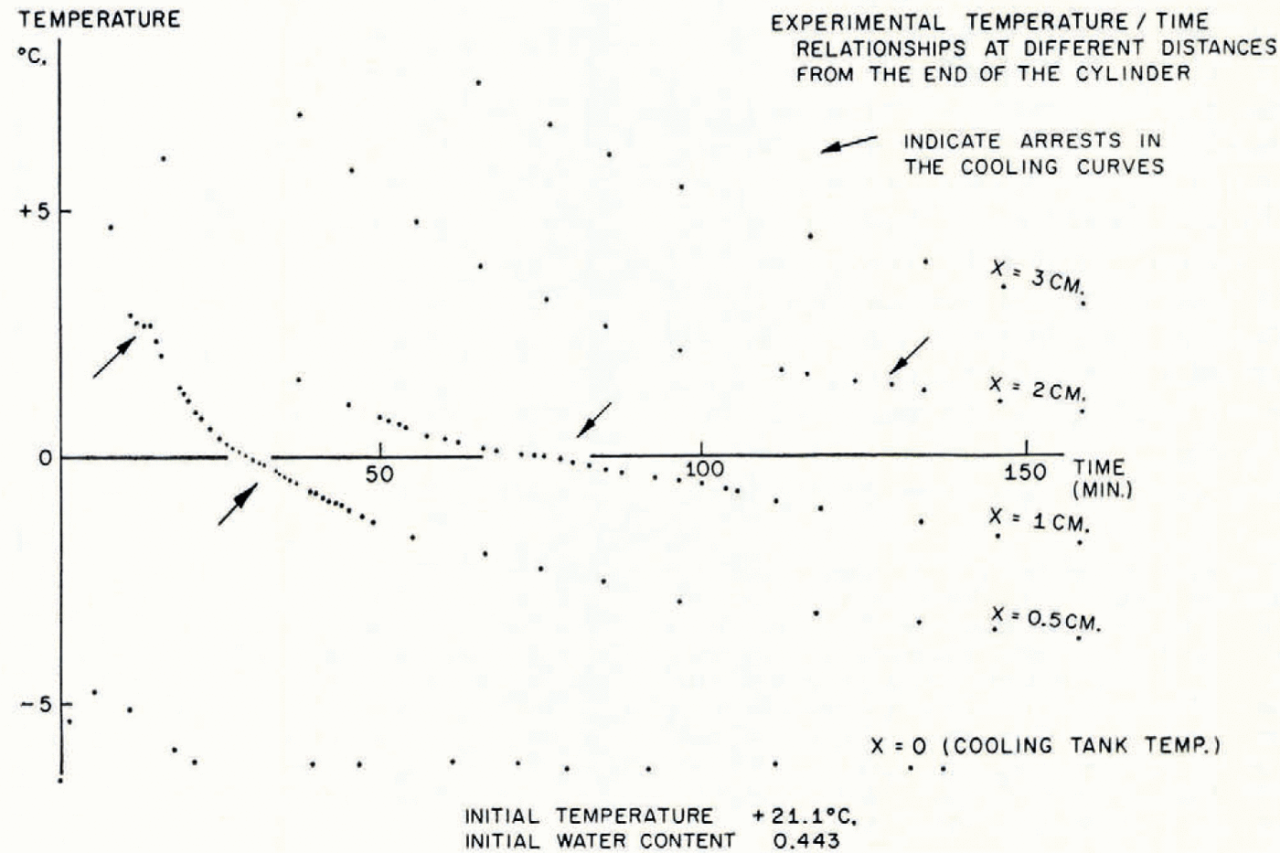
Fig. 5. Experimental temperature/time relationships at different distances from the end of the cylinder
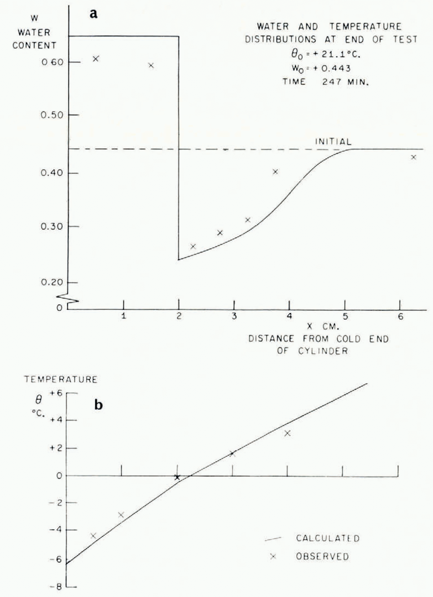
Fig. 6. Water-content and temperature distributions

Fig. 7. Water-content and lemperalure distributions
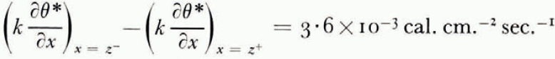
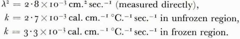
The thermal conductivity was not measured in these experiments, but estimated from the results of an extensive investigation by Kersten (1963), from which the conductivity for unfrozen Fairbanks silty clay loam, a soil slightly coarser than blue clay, is 2.7×10⁻³ cal. cm−1 °C−1 sec−1 at 4°C. and ω = 0.25. This can be taken as the conductivity of the unfrozen soil on the warm side of the freezing front. On the frozen side there are parallel layers of ice and of unfrozen soil with ω = 0.25, in such a way that the water content averaged over both soil and ice is 0.595. Neglecting contact thermal resistance between the layers and using standard values for the conductivity and density of ice, the conductivity of the frozen layer can be estimated as 3.3×10⁻³ cal. cm.−1 °C−1 sec−1. Comparing the measured terms in the heat-balance Equation (14) for the experiment illustrated in Figure 7,
and

which agree well.
As was pointed out earlier, this theory is unable to predict the smoothed temperature and ω fields unless either the rate of advance of the freezing front or the temperature at the freezing front is known. Using the measured rate of freezing-front advance, the temperature and ω fields have been calculated and are plotted in Figures 6 and 7. The following properties have been assumed:
Although mathematically convenient, it would be too severe an idealization to suppose the diffusion coefficient μ 2 constant, but its measured dependence on water content can be closely approximated by an exponential function of changes in ω, and a numerical solution for this case has been given by Reference CrankCrank (1956); the function of ω assumed is given in Figure 4. It might be thought that this computation would be made invalid by the circularity of determining k from the observed water-content field in one case. This is not so, because quite large changes in the assumed value of k have only a small effect on the calculated ω distribution, and large changes in ω have only a small effect on k.
The agreement between the observed and calculated temperature and w fields is quite close. These, of course, are the smoothed θ * and ω * fields. The ice-lens spacing depends on the perturbations close to the freezing front and it has not been possible to predict these. It was suggested earlier that a rough order of magnitude estimate of the distance between lenses is given by
More detailed knowledge of the nucleation process will be required for deeper understanding of the temperature and water-content histories close to the freezing front. Since the observed smoothed fields correspond to θ F at the freezing front about −0.4°C., the supercooling θ n which is available for lens nucleation must be much less than this, of the order of 0.1°C. In tests where small clay samples were cooled rapidly (at cooling rates of the order of 1 °C./min.) θ n was observed to reach much larger values before nucleation occurs, of the order of 2°C. This tends to support the earlier suggestion that the delay before nucleation is much longer when θ n is small.
Acknowledgements
The author is grateful to Professor D. C. Drucker for his advice and encouragement; to the National Science Foundation for support under Grant GP-1115 to Brown University during the period when the greater part of this investigation was carried out; to Mrs. N. Blinn and Mr. P. Rush for their assistance with the experimental programme; and to Dr. S. Takagi and Mr. C. Kaplar for helpful discussions.