


Introduction
Studies of the solar system by means of automatic interplanetary spacecraft have allowed us to extend our knowledge of the other planets. It has been found that ice is one of the most prevalent states of water. Large masses of water ice are contained on the surface of Mars and Pluto as well as (according to the comparison between reflection spectra and the H2O ice spectrum) on three of Jupiter’s moons and on six of Saturn’s moons. On the Earth about 90% of the total amount of fresh water is accumulated in giant glacial covers: almost all the water on Mars is contained, apparently, in its polar caps and in the thick layer of permafrost.
The enormous role of ice in forming the appearance of some planets offers a cosmological perspective in glaciology and opens a new direction for it – space glaciology, which is aimed at studying ice on other planets. It is these planets which will in the near future become objects of great attention as the bases for studying the solar system and space.
In this paper an attempt is made to summarize the available data on ice covers and ice on other planets on a scientific basis by using a mathematical approach, so that the phenomena observed may be explained and our ideas on the structure of these planets corrected.
The Amount of Water on Planets
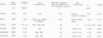
Table I summarizes the data on planets on whose surfaces ice has been discovered; this information has been taken from Reference MarovMarov (1981), Reference GehrelsGehrels (1976), and Reference MorozMoroz (1978). Brief descriptions of the characteristics of the ice cover of these planets are presented below.
Table I. Planets of the Solar System the Surface of which contain Ice
On Mars, as on the Earth, there exist giant polar caps. The atmosphere of this planet is very rarefied (the pressure at the surface is as low as five to six millibars); due to this fact, the surface temperature is far less than the freezing point of water, i.e. it is about 213 K on average. Typical temperatures of the polar caps are close to 150 K; the Viking-1 orbiter registered extremely low temperatures in winter – about 135 K in the region of the polar caps. In summer the following temperatures were registered: about 180 K in the region of the southern polar cap (Mariner-9 orbiter) and about 200 K for the northern one (Viking-2 orbiter). The condensation temperature of CO2 at pressure p = 5 mbar is close to 148 K. This allows us to suppose that the correct model for the Martian polar caps must be a two-component one (Reference MorozMoroz, 1978): H O ice in the permanent part and CO2 ice in the variable periphery. In summer the polar caps are intensively contracted (CO2 ice is sublimated), and in winter time the caps are enlarged (gaseous CO2 is condensed from the atmosphere). The mean thickness of this seasonal CO2 precipitation amounts to some fractions of a metre in the winter period; in this case the maximum mass of condensate in the seasonal caps is about one third of the mass of atmospheric carbon dioxide. The mass of the variable part of the southern polar cap at maximum is almost twice as much as that of the northern cap. This is consistent with the hypothesis of a two-component ice structure, since temperatures in the southern polar region are lower than those in the northern region, and the periods of formation of the polar caps are 382 and 305 d, respectively. At a minimum, when the variable peripheral part disappears, the southern cap is about 300 km across and the northern one about 900 km across.
According to Voyager IAS (Interplanetary Automatic Station) data, all the moons inside Titan’s orbit – Janus, Mimas, Enceladus, Tethys, Dione, Rhea – are covered with water ice. Their mean radii are 100, 195, 250, 525, 560, and 765 km, respectively. Judging by the fact that their mean density is close to that of water, one cannot exclude the possibility that some of these moons consist entirely of ice, and H2O ice is the major component in the remaining ones.
It was noticed long ago that Europa has the largest reflectance amongst the Galilean moons of Jupiter. The information obtained from Voyager-2 IAS allowed us to conclude that this celestial body has the smoothest surface among all the planets of the solar system: this planet, being comparable with the Moon in size, has maximum relief variations of the order of tens of metres only. At the same time, a great number of linear structures intersecting at different angles has been recorded on its surface, as well as bands having a thickness of some tens of kilometres on average, and a depth of some hundreds of metres, and also filament-like strips. These can be explained within the framework of a model according to which the effectively solid ice crust tens of kilometres thick rests upon a far thicker layer consisting of a mixture of friable “spongy” ice with water (sludge) (Reference MarovMarov, 1981). These two layers — the sludge (water-ice mantle) and the ice dome — form the upper envelope of Europa; its maximum thickness is estimated to be hundreds of kilometres. It is supposed that partial melting of the lower part of this envelope is caused by internal heat generation. Possibly, the water-glacial envelope of sludge hides, like an ocean, large variations in elevation of rock surfaces. The filament-like strips on Europa’s surface represent cracks in the solid upper ice dome, which arise under the effect of internal stresses where the sludge is expanded and contracted. The cracks are supposed to be filled-in with a fresh, lighter ice arising from up-welling sludge, which would explain the appearance of light bands on a relatively muddy surface of ice. Some dark substance is supposed to rise to the surface from great depths together with the sludge, so as to explain the presence of a system of dark strips (Reference MarovMarov, 1981).
The presence of water ice was also established on the other large Galilean moons of Jupiter, Ganymede and Callisto. The relatively low mean density of these planets testifies to a large H2O fraction in their mass.
Next we shall estimate the amount of H2O contained on the largest planets of the Earth group and on the Galilean moons of Jupiter.
There is no solid glacial dome on Mars; according to published scientific data (Reference CuttsCutts, 1973), the volume of water held as ice in its polar caps is estimated to be
which is approximately half that contained in the ice sheets and glaciers on the Earth. One supposes that much frozen water should also be contained in the thick layer of permafrost (Reference Kuz’minKuz’min, 1981), the signs of which have been recorded on the Martian surface as characteristic erosion forms by Viking-1 and Viking-2 IAS.
We can estimate the amount of frozen water held in this permafrost on Mars. The steady-state distribution of temperature T with depth z in the presence of a thermal flux q coming from the interior of the planet, can be represented by the formula
where λ is the thermal conductivity of rock and Ts is the mean temperature of the surface. The thickness of the permafrost layer Hp is estimated from the consideration that the temperature at its bottom reaches the melting point of ice

Assuming, as for Earth rocks, that λ = 2W m−1 K−1 and that the thermal flux from the Martian interior, like that for the Earth (Reference MorozMoroz, 1978), is q ≈ 4.18×10⁻²w m−2 (which corresponds to a temperature gradient in the upper layers of a lithosphere of about 20 deg/km), we obtain for a mean temperature of the Martian surface Ts ≈ −60°C (Reference Kuz’minKuz’min, 1981),
This value exceeds by a factor of 8 to 10 the thickness of a typical permafrost layer on the Earth. Reference Kuz’minKuz’min (1977) gives figures of the same order of magnitude, although admittedly differing appreciably. The temperature in polar regions is, on average, slightly below −100°C (Reference Davies, Davies, Farmer and La PorteDavies and others, 1977); however, Martian ice caps consisting mainly of water ice play the role of heat insulators. As an estimation using Equation (2) shows, under an ice layer 2 km thick the temperature of the bedrock increases by 40 deg as compared with the surface temperature for accepted values of λ and q (the gradient in an ice layer is c. 20 deg/km). The covering glaciations thus help soil conservation and protect soils against permafrost generation (Reference KrassKrass, 1983); this fact is well traced in the geological history of the Earth. In Siberian regions, which did not undergo deep glaciation, permafrost some 500 to 600 m thick developed. At the same time, the parts of Europe whose history includes more than one glacial epoch, have, apparently, never been subjected to permafrost. One should expect that under polar caps the permafrost layer is considerably less thick than that indicated in Equation (4). Only at sub-polar latitudes which are poorly screened against the cold by an ice sheet, can the permafrost be thicker. For these reasons CO2 ice is hardly present in Martian underground ice in any considerable amount. In the estimates which follow we shall take the average thickness of the permafrost layer over Mars as in Equation (4).
The volume of water contained as ice in a spherical layer of thickness Hp with an outer radius R equal to that of the planet is calculated to be

where Wc, is the relative content of H2O. For Wc = 0.2 to 0.3 (the mean water capacity of frozen soils on the Earth) the volume of water contained as ice in the Martian permafrost layer would be equal to (0.9 to 1.3) × 108 km3, which exceeds by two orders of magnitude the volume of H2O ice contained in the polar caps. Reference Kuz’minKuz’min (1977) gives a value for the total content of ice in the permafrost on Mars which is an order of magnitude lower than the one indicated. In this case the average thickness of the Martian permafrost would have to be only a tenth of that estimated by Equation (4): it would be as low as about 300 m. One might think that such an “Earth” figure could correspond to the severe Martian conditions, if one assumed that the deep thermal flux from the planet’s interior were considerably more than that in the Earth. This fact, however, does not agree with the ideas of modern planetology (Reference MorozMoroz, 1978).
Of definite interest is the estimation of the water fraction in the Galilean moons of Jupiter. For simplicity, we shall assume that these planets have a two-component composition: a light H2O component with density ρ, being in an outer layer of thickness h, and a heavy component which constitutes the internal part (the basic rocks) of the planet, with a mean density ρ1. Then, the total mass of the planet will be

from which the following expression for the thickness of the outer light H2O envelope is obtained:

We assume ρ1 = 3.5 Mg/m3, the same mean density as is attributed to the Galilean moon Io which, apparently, does not contain a noticeable amount of water. Then, using the parameters indicated in Table I, we obtain the following estimates for thickness of an outer envelope consisting of H2O for Europa, Ganymede, and Callisto:
The same value for hE is deduced by Reference Cassen, Cassen, Reynolds and PealeCassen and others (1979, Reference Cassen, Cassen, Peale and Reynolds1980). If one assumes that the mean density of the basic heavy componenent is the same as that on the Moon, i.e. ρ1 = 3.33 Mg/m3, then the estimates using Equation (7) are reduced as compared with these figures by approximately 25 to 30%. Table II shows the results of estimates of water content for the planets indicated above.
Table II. Estimates of H2O Content of Planets

The above values of total volume of water for the Earth and Mars may be increased if underground water is taken into account. First of all, it is interesting to note that the water content on the Galilean moons considerably exceeds the total amount of H2O on our planet: on Europa it is more than twice, on Ganymede and Callisto thirty times. Whereas for the Earth and Mars the fraction of free water in the total mass of the planet is negligible, it is rather significant for Jupiter’s moons. Recent publications (Reference MarovMarov, 1981; Reference SoderblomSoderblom, 1980) estimate the thickness of an outer envelope of Europa, consisting of ice and water-ice sludge, to be some hundreds of kilometres. This value, however, seems to be overestimated since, according to Equation (7), it requires the density of the heavy component (for a given mean density of the planet) to be ρ1 = 6 to 8 Mg/m3, which is evidently unjustified for a relatively small planet.
To evaluate the validity of figures characertizing the total water content of planets of the solar system which are given here and below, one should bear in mind that different forms of ice may exist. Figure 1 shows the phase diagram of H2O ice; it is generalized from the fundamental works of Reference BridgmanBridgman (1937), Reference Brown and WhalleyBrown and Whalley (1966), Reference Kamb, Rich and DavidsonKamb ([c1968]). Only the usual ice I has a density lower than that of water; the other structural forms of ice have higher density. As the pressure grows due to more dense packing of water molecules, not only does ice density increase, but the phase transition temperature also increases. Thus, at a pressure of 200 kbar the melting point for ice VII is about 440°C (713 K) (Reference FletcherFletcher, 1970). Each form of ice corresponds to its inherent field of stability in the (p, T)-plane, i.e. to the conditions of pressure and temperature.

Fig. 1. Phase diagram for H2O ice.
Table III gives the densities for the different forms of ice corresponding to Figure 1 given by Reference FletcherFletcher (1970). It can be seen from this table that the densities of the various forms of ice other than ice I exceed the density of water. However, the pressure and temperature conditions for the existence of these forms should be compared with specific conditions in the planets containing H2O in this or that form. Thus, according to Equation (8) for Europa the pressure at the bottom of the H2O layer hE does not exceed 1 kbar. Judging by the diagram in Figure 1, one would hardly expect that other forms of ice than ice I could exist at such pressures and for temperatures T > 100K. For Mars, with a mean rock density at the surface of about 1.5 Mg/m3 (Reference Kuz’minKuz’min, 1981) the pressure would not exceed 0.3 kbar even at the bottom of a 5 km layer, so that at temperatures T > −60°C only ice I should exist in this permafrost region. For Ganymede and Callisto the pressures in the ice or water envelope may reach as much as 10 kbar, and in this case the form of ice VI at T > c. 300 K may exist.
Table III. Densities for the different Forms of Ice

If one assumes, for example, that the ice density is, on average, 1.2 Mg/m3, (as in Reference Consolmagno and LewisConsolmagno and Lewis, 1976) rather than 0.9 Mg/m3, as has been taken in making estimates using Equation (8), then the thicknesses of the ice layers for Ganymede and Callisto hG and hC will increase by 15% as compared to Equation (8). However, one should take into account here that such an estimate is valid for the case where an outer layer has a relatively low temperature and is composed of ice only. On the other hand, if one assumes that, as a result of internal heating, these planets have been stratified up to the present time with the formation of a silicate core and a liquid water mantle, then corrections to Equation (8) will be considerably smaller, since ice II may exist, according to (p, T)-conditions, up to depths of 250 to 300 km only. A considerable increase of water fraction in the total mass of Ganymede and Callisto may take place only if ice VII with a density of 1.66 Mg/m3 exists in the internal central region of these planets where pressures reach 50 kbar and more. However, as follows from Figure 1, the temperatures in a core consisting of a mixture of silicates and ice should not exceed in this case the value of 400 to 450 K, which is not in agreement with calculations of the thermal evolution of the Galilean moons of Jupiter (Reference GehrelsGehrels, 1976) and corresponds to a cold state of their interior.
Hence, the estimates of water content on the other planets, given in Table II, are apparently close to the real values. It is a surprising fact that the amount of water on three of Jupiter’s moons exceeds the total H2O mass on the Earth by a factor of nearly 70. This fact becomes perhaps less mysterious if we take into account calculations of the lifetimes of volatiles in the solar system published some 20 years ago by Reference Watson, Watson, Murray and BrownWatson and others (1963). They show that, at heliocentric distances comparable to that of Jupiter’s orbit, volatiles like H2O are stable for periods exceeding the lifetime of the solar system. However at heliocentric distances such as those of the Earth and Mars, such volatiles can only survive on very massive planets, i.e. the terrestrial planets probably lost a great deal of their volatiles during the accretion phase.
Polar Caps of Mars
One may suppose, apparently, that during the period of summer sublimation of CO2, which comprises the variable part of the Martian polar caps, the caps of minimum size consist of water ice. From this viewpoint, it is of interest to estimate the ice-sheet thickness and the amount of ice on Mars. These estimates will be done using two methods which assume that ice domes composed of H2O are stationary.
The first method uses the idea that ice flows as perfectly plastic body. Integral estimations of the type which have been done for ice domes on the Earth, correspond satisfactorily enough (with 20–30% uncertainty) to the characteristics observed (Reference PatersonPaterson, 1969). We shall consider an axially symmetrical ice dome resting on a flat bed; one may show that the profile of a perfectly plastic glacier should in this case have a parabolic shape of the form

where H is the ice thickness at the centre where r = 0 and R is the ice-dome radius. The shear stress at the bottom is determined in the first approximation as

The mean value of a shear stress at the bed is

Substituting Equations (9) and (10) into this equation, we obtain
For the equilibrium state of an ice dome the condition
should be generally satisfied where τ0 is the yield point. The substitution of an expression for τ b determines H as a function of radius R:

The ice volume is then determined as

Assuming for ice τ0 ≈ 1 bar (Reference PatersonPaterson, 1969), and using the gravitational acceleration on Mars, gM = 3.71 m/s2 (Table I), the maximum thickness and mass of ice in the northern polar cap for which RN = 450 km are equal to
and for the southern polar cap for which RS = 150 km,
The total mass of ice in both caps is such that, according to Equations (13) and (14) the amount of water, recalculated per unit surface area of the planet, is equal to

This estimate shows the mean thickness of a water layer which would cover the Martian surface if the polar caps were melted provided that the relief of the planet were uniform. A close value (about 104 kg/m2) is indicated in the scientific literature on Mars studies (Reference MarovMarov, 1981; Reference CuttsCutts, 1973).
The second method for estimating the Martian ice domes is based on an ice model with a linear viscosity. For the mean thermal flux from the interior of Mars, estimated to have the same value, approximately, as that for the Earth, qm ≈ 4×l0−2 W/m2 and for an ice surface temperature of about 150 K, the mean temperature of the ice domes is about 200 K. This low temperature of the water ice in the domes can be maintained by the seasonal sublimation of the CO2 condensate from its surface with the consumption of a latent heat of condensation Q = 585 J/g. The effective viscosity of ice at such a temperature, as follows from the rheological law (Reference Grigoryan, Grigoryan, Krass and ShumskiyGrigoryan and others, 1977) with an exponential temperature dependence, µo exp (E/RT) with µo ≈ 1015 P (Reference ShumskiyShumskiy, 1969) is
At such viscosity it is advisable to consider the condition for the existence of an axially symmetrical, stationary glacial dome, which in the isothermal approximation has the form (Reference KrassKrass, 1983)

where a is the accumulation function. From this relation under the condition
we obtain the equation for a stationary ice cap in the form

where ξ and η are the variables over which the integration is performed. Assuming for simplicity that a = const, we obtain the approximate formula

According to Viking orbiter measurements, during the summer season over the northern polar cap of Mars the content of H2O in the atmosphere was found to be equal to about 80 µm of precipitated water; the maximum abundance of H2O, measured outside the polar caps, was equal to 30 µm of precipitated water. Probably, there exists some water circulation on Mars, where evaporation occurs according to the principle of freezing-out of the soil layer containing permafrost. The presence of water in the atmosphere is an essential argument in favour of a water-ice containing permafrost. The presence of water in the atmosphere is an essential argument in favour of a water-ice composition of the “permanent” domes of Mars. Apparently, in the autumn season, before CO2 condensation, precipitation of this liquid on the water-ice domes’ surface occurs. Assuming, in accordance with the measured quantities, the mean value of these precipitations to be a = (2 to 3)×10−10 cm/s, we obtain corresponding estimates of the maximum thickness for the polar caps of Mars:
In this case the volume of ice in a cap is determined according to Equation (18) by formula

With due respect for accepted numerical values of quantities composing this relation, the masses of Martian polar caps are in this case equal, respectively, to
Of course, the estimates (19) and (21) are rather approximate like the estimates (13) and (14); nevertheless, the corresponding values of ice volumes, found from these estimates, are nearly equal. The “viscous” ice dome is more gentle and elongated as compared to the “plastic” one.
Of interest is the estimate of temperature TB on a bed of Martian ice domes. The substitution of estimated values for HN and HS into Equation (2) yields the following results. In the case of the perfectly plastic glacier, since its height is greater according to Equation (13), the temperature of ice on the bed of the northern polar cap in the central region may reach the melting point. For the case of the viscous dome model TB≈240 to 250K, and ice is frozen to the bed. The southern polar cap does not have any basal ice melting region in either of the above models. The fluctuations of the deep thermal flux in the polar glaciation regions of Mars are, apparently, not so intensive that bottom ice melting and stream flow of ice as in the outlet glaciers on Earth can be caused (Reference KrassKrass, 1983). The photographs of the polar caps did not exhibit such formations (Reference MorozMoroz, 1978).
The polar caps of Mars are the so-called “indicators of history”: the “Viking” photographs (Reference Davies, Davies, Farmer and La PorteDavies and others, 1977) clearly show the existence of alternating dark and white layers of ice on the sections of terraced ledges. Traces of volcanic eruptions and seasonal dust storms, like the annual rings of a tree, were imprinted upon the “ice memory” of this planet.
Glacial Envelope of Europa
The purpose of the Section is to study the ice-cover dynamics for one of the most mysterious and astonishing moons of Jupiter. Floating ice domes are typical of the Earth’s polar regions as well; a considerable distinction from Europa consists in the thickness of ice armour, as well as in their continuity and temperature. The problem of their mechanics has been considered for the floating shelf glaciers of the Earth within the framework of ice creep (Reference SandersonSanderson, 1979) and non-linear viscosity with due respect for their temperature dependence (Reference Shumskiy and KrassShumskiy and Krass, 1976).
Such an approach is hardly valid for Europa in view of the continuity of its ice cover and the small variations of its surface elevation: here the main role should be played by oscillations of a floating ice envelope and stresses caused by the vertical temperature gradient within it.
Several recent papers show that there is some doubt concerning the existence of a water mantle on Europa under the ice shell (Reference Cassen, Cassen, Reynolds and PealeCassen and others, 1979) because tidal energy dissipation (1011 J/s) is insufficient to heat ice to the melting point. But in a later paper the same authors write: “The clean appearance of Europa’s surface, the very low topographic relief, the apparent scarcity of identifiable impact craters, and the network of curvilinear tectonic features all would be plausible consequences of a thin crust over liquid water” (Reference Cassen, Cassen, Peale and ReynoldsCassen and others, 1980). More correct calculations show that even the tidal dissipation in a thin shell can be sufficient to support the existence of a water mantle (Reference Cassen, Cassen, Peale and ReynoldsCassen and others, 1980).
The main parameters of Europa, used below, are taken from Table I. The densities of ice ρ and water ρw are assumed to be 900 and 1000 kg/m3, respectively. The schematic cross-section of the planet is shown in Figure 2.

Fig. 2. Schematic cross-section of Europa. 1 – ice envelope; 2 – water-ice mantle; 3 – basic rocks.
Thickness of the floating ice envelope
The temperature field of an ice crust when there is no ice flow due to small surface gradients, may be considered to be a steady one. Thus, one may use the solution of a stationary one-dimensional temperature problem in the form of Equation (2) with the given temperature TS at the envelope surface and thermal flux q at its bottom, generated in planetary interiors. The melting temperature Tm of ice I depends on a hydrostatic pressure,
where C0 = 7.28×l0−3 deg/bar is the coefficient of the change of melting point with pressure (Reference Shumskiy and GrigoryanShumskiy, 1982) and Tmo is the melting temperature of ice I under normal pressure. With due account for a zero pressure at Europa’s surface, we obtain from Equations (3) and (22) the formula for estimating the thickness H of the solid ice layer

where P0 is the normal pressure equal to 1 bar. Assuming that the thermal flux of Europa is of the same order as that on the Moon
we obtain H ≈ 20 to 25 km. The lower value of q ≈ 0.25×l0−3 J/m2 results in increasing H up to 85 km, according to Equation (23). In this case the ice melting temperature at the bottom of a solid crust is equal, according to Equation (22), to −2 to −3°C in the first case and about –8°C in the second. If we consider tidal heating the total surface heat flux can be as high as 5×10⁻² J m−2s−1 and in this case a liquid water mantle can persist (Reference Finnerty, Finnerty, Ransford, Pieri and CollersonFinnerty and others, 1981).
The above estimates confirm the validity of the supposition that Europa’s ice crust floats on a water-ice mantle whose state is close to a liquid one, and also testifies to a considerable role of temperature in the mechanics of this floating ice cover. This consideration results in a number of interrelated problems:
The proper oscillations of a floating ice crust; The stress state in such a crust caused by a stationary temperature field; The influence of temporary variations of temperature at the surface.
This cycle of problems should explain the principal features of the dynamics of Europa’s ice crust and the peculiarities of its surface relief.
The following remarks can be made concerning water-ice envelopes for Callisto and Ganymede. The variations of relief elevations of these moons of Jupiter are comparatively large (Reference GehrelsGehrels, 1976); well-conserved meteorite craters and large valleys are observed on their surfaces. Apparently, these planets are not subjected to active endogeneous processes leading to the internal heat generation. By virtue of this circumstance, one cannot exclude the possibilities that nearly all the water on Ganymede and Callisto is effectively in a solid state, as ice, or else the outer envelope of these planets is an ice crust some hundreds of kilometres thick, which is floating on a water mantle.
Temperature in the spherical ice envelope
In what follows we shall use spherical polar coordinates (r, Θ, ϕ) for the case of radial symmetry. In other words, we shall assume that the ice envelope, floating on a liquid substrate, is uniform in thickness. Generally speaking, since the latitudinal variations of temperature at Europa’s surface reach some tens of degrees (Reference SoderblomSoderblom, 1980), then, according to Equations (23), the corresponding variations of thickness of a solid ice armour may reach 10 to 15% of its mean thickness. We shall neglect this non-uniformity in order to simplify the problem and shall consider further the radially symmetrical scheme only with variations limited to one coordinate directed along radius r.
The stationary temperature field in the ice envelope (in the absence of heat sources) is described by the equation

The boundary conditions are: temperature Ts is specified at the surface as
and the melting temperature is specified at the bottom of the solid envelope as
The solution to Equations (24) to (26) is given by
Equation (27), as well as Equation (23), were obtained for the case where the thermophysical parameters are constant. In actual fact, they are temperature dependent. Thus, the heat capacity CP varies almost linearly within the temperature range 50 to 270 K (Reference Giauque and StoutGiauque and Stout, 1936). The dependence of thermal conductivity λ on T has been studied by Reference KlingerKlinger (1975), Reference Andersson, Andersson, Ross and BäckstrӧmAnderson and others (1980), and Reference Klinger and RochasKlinger and Rochas (1982). The curve of the dependence of λ on T has a maximum at a temperature below 10 K and decreases as temperature increases.
In Equation (27) the ice melting temperature Tm at the bottom of the solid crust (for ice I) is determined by a formula similar to Equation (22) with a correction for zero pressure at the surface,
Along with a stationary (in the accepted approximation the radially symmetrical) temperature field, resulting from the long history of the planet’s existence, there is also a temporal component caused by at least two time variations of temperature at Europa’s surface: from the period of revolution around Jupiter, td = 3.55 Earth days, and from the sidereal period with the duration ts = 11.86 Earth years. The attenuation decrement of osciallations at frequency ωi, generated at the surface of a homogeneous medium with temperature diffusivity k, is determined by the penetration depth hi estimated by equation (Reference Carslaw and JaegerCarslaw and Jaeger, 1959)
Table IV gives values of hi (in metres) for different values of k (m2/year) and ti = 2π/ωi.
Table IV. Penetration Depths of Thermal Fluctuations

The table shows that in a wide range of possible variations of thermophysical parameters of ice, the temperature effects caused by variations with a period td influence a thin near-surface layer having a depth of up to one metre only; the depth of action of sidereal variations does not exceed, apparently, some tens of metres.
In connection with the existence of considerable temperature gradients in the depth of ice, the problem of studying the temperature dependence of properties of this material arises, the temperature being varied within wide limits - from very low absolute temperatures up to the ice melting point under the normal conditions. This problem is very complicated and multi-facetted, particularly in its experimental aspect. At present, the temperature dependence of the coefficient of linear expansion for ice α is known confidently enough (Reference ForsytheForsythe, 1954; Reference VagaftikVagaltik, 1956).
The last two columns in Table V represent values calculated by approximation formulae for α of the first (P1) and second (P2) orders respectively, obtained by the least-squares method using the values given in the first two columns of the Table:
where α0 = 10−6 deg−1. As Table v shows, the coefficient of linear expansion for ice is strongly dependent on temperature. This fact, by itself, shows how complicated experimental work with ice at low temperatures is.
The elastic characteristics of polycrystalline ice slightly change with temperature: when the temperature changes from 0 to −180°C, the Young’s modulus increases by 10% at constant load (Reference Zarembovitch and KahaneZarembovitch and Kahane, 1964). In solving the problems below we shall assume the main elastic characteristics of ice, the shear modulus G and Poisson’s ratio v, to be constant. In particular this assumption is quite justified for v: it is well known that v is almost independent of the ice structure and equals 0.33. As far as the shear modulus G is concerned, it strongly depends on the structure and, hence, on the temperature of ice; however, there are no reliable data on this dependence. Therefore, by assuming G = constant, we mean that an average value of this parameter is used.
Table V. Dependence of Linear Expansion coefficient of Ice on Temperature

Free oscillations of an ice envelops
We shall consider two types of oscillations of a floating spherical ice envelope in the self-gravitational field of a planet, radial (the simplest type of spheroidal oscillations) and torsional. Similar problems have been solved in theoretical geophysics as applied to the analysis of the proper oscillations of the Earth (Reference MagnitskiyMagnitskiy, 1965, Reference JeffreysJeffreys, 1970); for this reason, the detailed derivation of the basic relations is omitted here. Temperature effects are not considered in the analysis that follows.
Radial oscillations
In the case of a radially-axial symmetry only one elasticity equation (Reference LoveLove, 1927) is retained, namely, the equation containing differentiation with respect to coordinate r (without taking into consideration the planet’s rotation)

Here u is the displacement along the radios r, W is the gravitational potential, and σii are stresses determined by the equations

In Equations (33) p is the pressure determined from a hydrostatics law

The boundary conditions of the problem are as follows. On a free surface the normal stress is zero
On the lower surface the Archimedean floating condition
is met. The condition of absence of tangential stresses on both surfaces is automatically satisfied by virtue of the radially-axial symmetry of the problem.
We substitute Equations (33) and (34) into Equation (32). With due respect for the expansion of the potential W
where W0 is the non-perturbed potential and δW is the perturbation (Reference MagnitskiyMagnitskiy, 1965), as well as the self-gravitating sphere conditions

we obtain, similarly to Reference Pekeris, Jarosch, Benioff, Benioff, Ewing and HowellPekeris and Jarosch (1958), an equation in terms of the displacement u,

In relations for δW and g, f is the gravitational constant. The solution to Equation (37) is sought in the form
Substitution into Equation (37) yields the equation for the function u(r) (Reference MagnitskiyMagnitskiy, 1965)

where in our case

After substituting Equations (33), (34), the boundary conditions (35) and (36) areas follows:


Equation (38) has two linear independent solutions in the form of the Ressel functions of semi-integer order (Reference MagnitskiyMagnitskiy, 1965; Reference Pekeris, Jarosch, Benioff, Benioff, Ewing and HowellPekeris and Jarosch, 1958),

The general solution to Equation (38) can he represented as
where C1, and C2 are constants to be determined. We can do this by substituting Equations (43) and (42) into conditions (40), (41). In order that the non-trivial solution of a system of two linear homogeneous algebraic equations in C1 and C2 exist, its determinant should be zero, i.e. the equality

has to be satisfied. This equation may be written in dimensionless form as

where

Equations (44) and (45) include the following dimensionless parameters of the problem:

In this notation the dimensionless thickness of an envelope is equal to γ – 1.
Let x1 = l1Rs be the smallest root of Equation (44). In order that instability of radial oscillations of a solid spherical envelope take place, the condition
should be met, or, as follows from Equations (39) and (46),

Then one of the multiplier exponents in the u(r,t) solution is positive, i.e. the radial displacement grows indefinitely with time. Some estimates are given below. As has already been mentioned above, the problem has been solved for the case G = const. At an ice temperature of the order of −20°C the Young’s modulus E = 2G(1+v)≈1010N/m2 (Reference Bogorodskiy and GavriloBogorodskiy and Gavrilo, 1980), i.e. for f = 6.672×10⁻¹¹ Nm2/kg2, m ≈ 1. For G values which are an order of magnitude lower we have m ≈ 3.
We shall now analyze the dependence of the least root x1 of Equation (44) on the parameters of the problem, namely β (the rigidity parameter) and γ (the envelope thickness parameter). The plots of x1(β) are shown in Figure 3. As the rigidity parameter β increases, x1 also grows. Within the possible range of Young’s modulus E (109 N/m2<E<9×109 N/m2) it follows from Equation (46) that
For the interval of values β < 0.05 the root x1 at β ≈ 0.05 is less than unity for γ < 1.03 and, hence, instability of proper oscillations of an ice envelope may take place. Figure 4 gives the dependence of x1 on the thickness parameter γ of a floating solid envelope. When the ice cover thickness increases, the stability of its oscillations grows; at γ > 1.03 the instability of osciallations for β < 0.05 is practically absent. In other words, very thin ice envelopes, floating on a liquid substrate, undergo unstable radial oscillations which lead to a breaking down of continuity. On the contrary, covers which are thick enough are less subject to destruction due to their proper radial oscillations, even if the shear modulus G is relatively low, i.e. very thick floating envelopes are most secure.

Fig. 3. Dependence of the root x1 of Equation (44) on β. Curves numbered 1,2,5,4,5,6 correspond to γ = 1.02, 1.03, 1.04, 1.05, 1.06, and 1.07 respectively.

Fig. 4. Dependence of the root x1 of Equation (44) on the ice envelope thickness parameter, γ. Curves numbered 1,2,3,4,5,6,7 correspond to β = 0.02, 0.03, 0.05, 0.08, 0.1, 0.15, and 0.2, respectively. The dashed lines show values of m calculated from Equation (47).
The dashed lines in Figure 4 show the values of m calculated by Equation (47) for β = 0.02, 0.033, and 0,05. The sections of the correspondence curves lying below these lines correspond to unstable oscillations, and those lying above the lines to stable ones. The points of intersection of one-parameter curves and direct lines divide the region of radial oscillations into stable and unstable parts. At β = 0.08, m = 1.72, so that when β > 0.08 the sections of all curves for 1<γ<1.07 fall within the unstable region. In other words, a decrease of “rigidity” of the floating envelope material (an increase of “pliability”) leads to an extension of the region of instability of its oscillations.
According to estimates made above, the thickness of Europa’s envelope for the case of the same interior thermal flux q as on the Moon is 20 to 25 km. When the value q is an order of magnitude lower than that on the Earth, this thickness increases up to 85 km. The mentioned values correspond to the following values of γ:
For γ1 at β ≈ 0.032 which corresponds to the acceptable value of E ≈ 8.8×10⁹ N/m2 for ice (Reference Bogorodskiy and GavriloBogorodskiy and Gavrilo, 1980), according to Equation (47), m = 1.1. The unstable section in curve 2 is within 1<γ<1.015, i.e. an envelope of up to 25 km thick undergoes unstable aperiodic motions; a thicker spherical ice cover oscillates in a stable mode.
As has already been noted, the whole surface of Europa is covered with a dense grid of cracks and fractures, many of which are quite long; this is clearly seen on photographs which show surface fragments transmitted from Voyager-2 IAS (Reference SoderblomSoderblom, 1980). Based on the above calculations and assuming that the mechanism of destruction of an ice envelope floating on a water-ice mantle is valid, due to the instability of radial oscillations for some particular combinations of basic parameters, at E ≈ 9×10⁴ bars the value of 20 to 25 km seems to be more acceptable for an ice-cover estimation.
It is also of interest to calculate the periods of proper radial oscillations of an ice envelope within the stable region. Table VI gives the values of first periods of these oscillations calculated according to Equations (39) and (46), by using the equation

For an envelope 25 km thick with a Young’s modulus E ≈ 90 000 bars (2G = 6.6×10⁹N/m2), the first period of proper radial oscillations is
As G increases the first period decreases and vice versa; for a relatively low values of G the period can be as much as several hours; as the shear modulus further decreases, the oscillations become aperiodic (unstable). The values of the second roots, as follows from the asymptotic form of Equation (44), are calculated approximately by the equation
It is seen that for γ ≈1 the values of the second roots are of the order of some tens and hundreds; in this case the second periods of proper oscillations are as low as a few seconds, which makes no physical sense.
Table VI. Fundamental Periods of the proper Radial Oscillations of the Icy Crust of Europa

As seen from Equations (46) and (47), when the planet’s radius Rs and mean density ρ increases, β and m become larger. This means, according to Figure 3, that the region of instability of radial oscillations is considerably extended. For example, on a planet like the Earth, a floating continuous ice cover some tens of kilometres thick would necessarily be crushed as a result of its proper aperiodic radial oscillations. Thus, the ice envelopes of relatively small planets are more stable and secure in the sense of their integrity.
Torsional oscillations
A similar problem was considered in theoretical geophysics as applied to the proof of existence of a liquid core in the Earth under the spherical layer of the solid mantle (Reference ShlangerShlanger, 1959).
Under torsional (toroidal) oscillations, volumetric strain is absent so
Only one equation of the system of elasticity equations remains since, by the definition of torsional oscillations, we have
The remaining component of displacement is represented in the form
The torsional oscillations are related to shear deformations and affect the rigid floating envelope only, i.e. the boundary conditions are of the form
or

Substituting Equation (50) into a single elasticity equation
we obtain, by using the method of separation of variables, the system of two equations with respect to w(r) and ϕ (Θ):


Equation (53) is the differential equation of spherical functions, i.e.
Equation (52) can be reduced to the Bessel equation; its solution is of the form (Reference Tikhonov and SamarskiyTikhonov and Samarskiy, 1966)
where k2 = pω2/2G. The following recurrence equations are valid for xn and ψn functions:

The substitution of Equations (55) and (56) into the boundary conditions (51), along with the requirement of the existence of a non-trivial solution for An and Bn yields an equation which determines k and, hence, the frequency ω (Shlanaer, 1959):

For n = 1 we obtain from Equation (57) the transcendental equation with respect to x = kRs in dimensionless form

where δ = γ−1 = Rb/Rs. Far δ close to unity, as well as for small values of x(1-γ) we have from Equation (58) the approximate equation for determining some first roots
Table VII gives the values of three fundamental periods of torsional oscillations for γ ≈ 1 correspondingly to the roots of Equation (59):
calculated from the equation

Table VII. Fundamental periods of Torsional oscillations of the floating Icy Crust of Europa

It is seen from Equation (60) and this Table, that a decrease of shear modulus of the material results in an increase of the period of torsional oscillations of the floating solid envelope. For the values of the basic parameters of Europa’s ice cover assumed above, the periods of the first harmonics apparently do not exceed 15 to 20 min. In this case the planet’s radius is linearly dependent on the value of the period.
Thermoelastic state of an envelops
To determine the deformations and stresses arising in a floating ice cover due to the inhomogeneity of its vertical temperature profile, we shall consider the boundary-value thermoelasticity problem for a radially symmetrical case. The temperature variation along the radius is described by Equation (27). At the bottom of the envelope, for r = Rb, the ice temperature at the melting point TM is determined by Equation (28); the temperature TS is specified at the free surface.
A single equilibrium equation is of the form

The stresses σii are determined as follows (the thermo-elasticity relations (Reference Melan and ParkusMelan and Parkus, 1953):

where the components of the strain tensor and the volumetric strain are determined by Equation (33). The substitution of Equations (62) and (33) into Equation (61) leads to the equation for a radial displacement

where α = α (T). Upon double integrating we obtain the expression for u(r)

where C1 and C2 are constants determined from the boundary conditions. The boundary conditions of the problem are determined as follows. On the free upper surface the normal pressure from a displacement u of opposite sign is specified as
On the lower surface, the hydrostatic equilibrium condition (Archimedean floating)
should be met.
We introduce the dimensionless variables

The problem of Equations (63), (65), and (66) is solved in two versions: for constant coefficient of linear expansion of ice α and for the case where this value depends on temperature according to Table V. For the second version the approximate dependence in the form of the second order polynomial given in Equation (31) was used; this dependence is written in dimensionless form as
where a = 82.885, b = 9.9225, T0 = 0.2446; here T is the dimensionless analogue of Equation (27):

The use of boundary conditions (65) and (66) yields the formula for u (in the dimensionless expression the rule over the dimensionless variables is omitted for the sake of simplicity).
In the general case the solution of Equation (64) is of the form

where

In the case of a constant coefficient of linear expansion, α = const, the function fT(r) in Equation (71) is expressed as

In the case where α depends on temperature according to Equation (68), the solution to the problem of Equations (63), (65), and (66) is also expressed by Equations (7), (71), but here the function fT has another form, namely,

It was assumed in calculations: for α = const = 5×10⁻⁵ deg−1; for α = α (T), α0 = 10−6 deg−1 (according to Table V); Ts = 0.34 (93 K is the temperature in the terminator region (Reference SoderblomSoderblom, 1980)). Tm was calculated according to the dimensionless analogue of Equation (28).
Figure 5 shows the dependence of the corresponding dimensionless deformation
on β and γ. Curves (β, ∆u) grow with β more noticeably as γ increases. The growth of ∆U with increasing β means that as the “rigidity” of an envelope material decreases, the thermoelastic deformations in it increase. The increase of thickness of a floating ice cover should lead to the growth of its corresponding deformations almost according to a linear law. The dependence of the coefficient of linear expansion of ice on temperature lowers ∆u by 30 to 40% as compared to when α = const; the gradients also decrease, i.e. all curves are more gentle for the case of α = α (T). Apparently, the situation which allows for the α (T) dependence is more realistic; the results of calculations for this version will be preferred in the interpretation that follows. For the values of the basic parameters of Europa, indicated above, β ≈ 0.2 according to Equation (67) and, as follows from curve 1, the corresponding radial thermoelastic deformation of an ice envelope may reach 2×10⁻⁴ of the planet radius, or about 300 m.

Fig. 5. Dependence of relative deformation Us – Ub, on β (curves numbered 1,2,3 correspond to γ = 1.015, 1.04 and 1.06) and on γ (curve numbers 4,5,6 correspond to β = 0.02, 0.05 and 0.2).
I: −α = const; II: – α = α (T) according to Equations (31), (68).
The increase of thickness of a floating ice cover leads to the increase of deformation and its gradients. Figure 6 shows the dimensionless dependences of stress σϕϕ and stress intensity τ on radius. These dependences are normalized with respect to the value E = 2×10¹¹ N/m2 and calculated from the Equations

In the case of α = const, σϕϕ varies with radius by a law close to linear; for α = α (T) deviations from a linear dependence are observed. The thermoelastic stresses for α = α (T) are negative at the bottom of a floating envelope and positive at the free surface. As the shear modulus decreases (β increases) the stress lowers, i.e. as the “pliability” increases, the thermal stresses in an ice crust decrease. The α (T) dependence has a considerable effect on the depth distribution and values of stresses: the gradients are much larger as compared to the α = const version. As β increases, the zero surface for σϕϕ and the minimum of τ are noticeably shifted towards the free surface: whereas for β = 0.01 the σϕϕ = 0 surface occurs almost in the middle, for β = 0.2 it is situated at a distance from the free boundary, r = 1, equal to only one tenth of the thickness of the rigid layer. For small values of β the stresses are rather high; for β = 0.2 they are about 10 to 20 bars. As the envelope thickness, γ - 1, increases, the stresses vary insignificantly provided β remains the same. The values of stresses at the bottom of a floating envelope are considerably higher than those on the free surface; thus, for γ = 1.015 (which corresponds, as has already been mentioned, to an ice cover 25 km thick) these values differ by a factor of 3 to 4. As follows from the curves of the series, the lower portion of an ice crust undergoes compression in the Θ and ϕ directions and the upper (in particular the near-surface) region undergoes extension.

Fig. 6. Thermoelastic stresses in an ice crust. γ = 1.015. a: – σϕϕ, b – τ.
I: – α = const; II: – α = α(T). Curves numbered 1,2,3, correspond to β = 0.1, 0.2, and 0.5, respectively.
Figure 7 shows the dependence of σϕϕ and τ on β for various internal spherical surfaces in an ice crust. For the currently accepted value of Young’s modulus for ice (β = 0.2) the thermoelastic stresses do not exceed 10 to 20 bars. This value is close to the spalling strength of ice; at the free surface, as has been mentioned above, these stresses are three to four times lower. The role of increasing β (decreasing Young’s modulus) in lowering the influence of a temperature inhomogeneity on the stress state of an ice armour is clearly seen in this case.

Fig. 7. Dependence of thermoelastic stresses on β.
γ = 1.02.
I: – α = const, II: – α = α(T). a: – σϕϕ, b: −τ. Curves numbered 1,2,3, correspond to r = 1/γ, 0.5 (1 + 1/γ), and 1, respectively.
Reasons for Europa’s surface relief peculiarities
As has been noted above, the main possible reason for the numerous cracks and giant fractures occurring in Europa’s surface is the instability of natural oscillations of an ice crust floating on a water-ice mantle. The ice envelope is literally crushed into separate blocks (Reference SoderblomSoderblom, 1980); an apparent absence of regularities and the chaotic character of the location of these numerous traces of the break-up of an ice armour on the planet’s surface proves the validity of the stated supposition. One cannot also exclude the possibility that one of the reasons for the break-up of the ice crust may consist in the influence of periodic perturbations from Jupiter and its other moons being in resonance with some of the frequencies of a spectrum of natural radial oscillations of Europa’s solid ice envelope. To answer this question finally, the problem of Equations (32), (33), (34), (35), and (26) should he considered while specifying the law for the variation of the shear modulus G and ice density ρ with radius r; these data could be obtained from the corresponding experiments. Of course, the eigenvalue problem can be solved in this case only by numerical methods. In a simplified formulation (with G and ρ constant) the problem of forced oscillations of an ice crust can be solved by analytical methods which can allow the calculation of the resonance frequencies and amplitudes.
Reference Cassen, Cassen, Peale and ReynoldsCassen and others (1980) advance thermal convection in the water mantle of Europa as the main reason for the break-up of the ice crust. However it is well known that thermal convection only takes place in the case of a pure and extremely homogeneous medium. Estimates show that density inhomogeneities of as little as c.0.01% are sufficient for thermal convection not to occur. It is doubtful if the real natural medium is that pure. Furthermore thermal convection would inevitably produce rapid cooling of the planetary interior.
Reference PieriPieri (1981) has described two types of patterns of fracture polygons on Europa’s surface: (1) roughly equal polygons and (2) complex trapezoidal patterns. These classes form distinct groups, often localized; but also some of global character.
Reference Finnerty, Finnerty, Ransford, Pieri and CollersonFinnerty and others (1981) suggest a model for the cracking of a thin, brittle crust floating on a water mantle 270 km deep in which it is due to the dehydration of enclosed serpentine which provides stresses great enough to fracture the ice on Europa. However there are two difficulties with their model: the thickness of Europa’s H20 layer is only c. 100 km and so the high temperatures (c. 500°C) needed for the dehydration of serpentine seem unrealistic.
Apart from the fact of the existence of fractures and crack systems in Europa’s ice crust as such, the analysis of their dynamics is of definite interest.
The thermoelastic stresses in a floating ice crust due to the existence of a temperature gradient in it, which may reach 7 to 8 deg/km, may be as high as tens of bars. True, under the conditions of considerable hydrostatic pressure, the gradient of which in an ice layer is 12 bar/km in the conditions prevailing on Europa, ice may change its structure and its mechanical characteristics. The ice structure may also be considerably reconstructed as a result of a long period at low temperature.
One of the most effective factors influencing the planetary surface is temporal variations of temperature. The amplitude of the diurnal temperature variations at the surface is about 100 deg (Reference GehrelsGehrels, 1976), the minimum value of the temperature on the night side of a planet being equal to only some tens Of Kelvins. As follows from Table IV, when the temperature drops below 70 K, ice begins to expand; for temperatures of the order of 10 to 30 K the total relative expansion of ice when cooling may be about 2×10⁻⁴. On the other hand the minimum temperature on the night side could be close to 50–70 K if we take into account the thermal inertia J = (λpc)½, albedo, and radiation. The larger J, the higher the night temperature will be and the more the day maximum temperature will be retained. In this case temperatures well below 60 K may occur only in the subpolar regions of the planet.
For a sufficiently large distance between the crack systems (of some tens of kilometres) such an expansion is large enough for filament-like cracks some tens of metres wide, which were opened on the day side, to be closed from the surface in the nighttime. For cracks some hundreds of metres wide and larger, the closing process, if any, has to be caused, apparently, in other ways. It is well known that closed cracks in an ice layer are observed from space as dark regions due to their decreasing albedo against the surrounding surface background. This factor is used for forecasting surges of glaciers on Earth from satellite data: prior to surges glaciers are usually covered with a grid of internal cracks, and their albedo sharply decreases. Of course, the process of closing cracks on the night side of a planet at temperatures of some tens of kelvins, as well as the process of their subsequent opening on the day side and narrowing due to the reversal of sign of the coefficient of linear expansion α, depend considerably on the latitudinal position of the crack system, because the angle of inclination of Europa’s rotation axis to the ecliptic plane is close to zero. Unlike the Earth, there are, apparently, no noticeable “winter” and “summer” temperature variations on this plant; the sidereal change of seasons plays a far greater role here. The set of major temperature harmonics, in which the diurnal and sidereal components play a considerable part, defines a complicated history of crack dynamics in the near-surface layer some tens of metres deep.
Consider the depth distribution of the thermoelastic stresses arising in the near-surface ice layer due to short-period oscillations of temperature at the surface of an ice envelope. In the preliminarily stressed state, caused by a stationary temperature field, it is the short-period oscillations which cause the appearance of systems of cracks in the uppermost layer of an ice cover. Since the periodic oscillations of temperature rapidly decrease with depth, it is sufficient to consider a one-dimensional problem with a variable z in the vertical direction. Under an assumption of independence of thermophysical parameters with temperature, the thermal-conductivity equation is of the form

where k is the thermal diffusivity. On the free surface the temperature perturbations Θ is specified as a harmonic with frequency ω and amplitude A0:
In addition, the condition that the perturbation decreases with depth is necessary, i.e.
The solution of Equations (76), (77), and (78) (temperature waves) is given by (Reference Carslaw and JaegerCarslaw and Jaeger, 1959; Reference Tikhonov and SamarskiyTikhonov and Samarskiy, 1966)

We shall now consider thermoelastic stresses arising due to the propagation of temperature perturbations from the surface to the depth. When the horizontal gradients are neglected, the thermoelasticity problem is also one-dimensional. A single equation of quasistatic equilibrium yields, with a zero value for the normal stress at the free surface taken into account,
since

it follows from Equation (80) that
and then from Equation (81) we obtain

In Equation (82) we consider α = α (T) according to Equation (31), which represents the data of Table V. In our case this dependence is of the form
where Ts is the time-averaged temperature of the surface, and T0, a, and b are the coefficients of Equation (31). The substitution of Equation (83) into Equation (82) leads to the dependence of the horizontal stress on the perturbation Θ, determined by Equation (79),

The test for an extremum leads to two equations


Equation (85) is valid for the case α = const as well; here the absolute maximum of σxx is reached at the boundary, for z = 0. By virtue of the relation between a and b, for Ts > T0 Equation (83) has two roots of opposite sign, i.e. the absolute maximum of σxx is reached for z > 0. This means that when the coefficient of linear expansion of ice depends on temperature, the maximum tensile stress from periodic oscillations of surface temperature may be reached at some depth. Thus, under some conditions the cracks may arise inside the ice; this phenomenon is well known in the freeze cracking of soils as “blind cracks”. These cracks do not reach the surface, but, by virtue of the fact that α (T) increases with temperature, can develop into the depth. As has already been mentioned, these surface regions with internal cracks, when observed visually from space, are viewed as dark stripes, and the alternation of opened and closed cracks as intermittent light and dark systems of stripes.
We shall now estimate possible uncompensated variations of a floating ice envelope’s relief. It follows from the balance equations that the horizontal (σxx) and vertical (σzz) stresses in a thin layer are related by an approximate dependence
where L is a characteristic linear dimension. In our case
where δ is the amplitude of an uncompensated elevation. If ![]() is the compressive strength of ice, then the extremal value of δ is estimated as
is the compressive strength of ice, then the extremal value of δ is estimated as

The characteristic linear dimension L of blocks of Europa’s crust is of the order of some hundreds of kilometres (Reference SoderblomSoderblom, 1980). Assuming L ≈ 100 to 200 km, h ≈ 25 km, we obtain that for σ°xx < c. 10 bars (Reference ShumskiyShumskiy, 1969) the extremal value of an uncompensated elevation may be some tens of metres. This value is in good agreement with the heterogeneities of the observed surface relief of Europa (Reference SoderblomSoderblom, 1980).
As far as the global dynamics of the crack systems in the floating ice armour of Europa in which the opening and closing of large cracks and fractures are concerned, probably, in this case, one should consider the problem of forced oscillations of an ice envelope with periodic perturbations from Jupiter’s gravitational field and its other satellites taken into account.
Conclusion
An exclusive role for ice in forming the appearance of Jupiter’s and Saturn’s satellites has been emphasized in the science literature of recent years. Reference PoirierPoirier (1982) considers the complex rheology of ice to be the key to the tectonics of the ice moons of the giant planets. One cannot disagree with this statement; however, we should not restrict ourselves to the study of ice rheology at low temperatures and high pressures; in order for research on the surface dynamics of these planets to be successful, an approach based on ice thermomechanics is necessary. Such a theory has been successfully developed and applied to studying glaciers on the Earth (Reference ShumskiyShumskiy, 1969, Reference Shumskiy and Krass1982; Reference Grigoryan, Grigoryan, Krass and ShumskiyGrigoryan and others, 1977; Reference KrassKrass, 1981, Reference Krass1983).
The necessity of broad experimental and theoretical studies of the variations of the mechanical and thermophysical parameters of ice, as well as of the reconstruction of ice structure at very low temperatures and high pressures, is now of particular importance. On this basis, one would be able to make fundamental advances in the theory and refine our ideas about the ice moons of Jupiter and Saturn as well as about ice covers on other planets of the Solar system.
The problems considered in this paper allow us to draw a number of conclusions on the role of water ice in the physics of the planets of the solar system.
-
1 Definition of the water volume on the planets is connected with the problem of their interior structures (Reference Consolmagno and LewisConsolmagno and Lewis, 1976). Approximate estimates are given in the paper; when a new model has been constructed these values will be capable of being defined more precisely. Europa contains H2O as about 5 per cent of its volume. More than one-third of the volume of both Ganymede and Callisto consists of H2O.
-
2 Mars is a typical terrestrial planet according to the relative amount of water. Most of its volume of H2O is contained as ice in permafrost, of which the mean thickness is about 3 km. Liquid water may occur under the permafrost layer. The Martian polar caps contain only about one per cent of the whole amount of water of the planet. The ice sheets of the Earth, by comparison, contain about 90 per cent of the volume of fresh water.
-
3 The thickness of the ice crust and liquid water mantle of Europa are 25–30 km and 60–80 km respectively. The relatively thin, floating, rigid envelope is broken up by its unstable radial oscillations. Probably this is the main reason for the formation of the fracture system on the surface of the planet.
-
4 The thermal stresses in the floating ice shell of Europa can play an important role in the dynamics of the ice shell and the pattern of the system of fractures.
-
5 Probably all of the water on Ganymede and Callisto consists of various forms of ice, i.e. tidal energy dissipation provides insufficient heat to melt their ice crust.
Some speculation can be made on the scientific investigations now desirable. It is necessary:
-
(a) to develop new rheological models of ice taking Into account the properties of ice at low temperatures and their temperature dependence;
-
(b) to create models of ice thermomechanics which are suitable for application to the surface dynamics of planets containing ice;
-
(c) to study the properties of “ices” of other substances and their role in the complex interaction with water ice.
The study of ice on other planets will allow us to gain new insights into the glacial covers of the Earth, and the conditions of their formation, as well as into the past glacial epochs on our planet.
Acknowledgements
The author thanks Professor P.A. Shumskiy for useful discussions.


