


1. Introduction
Antarctic ice tongues are the floating end of one or two main input glaciers; they tend to be much longer than wide and are not constrained by topography (Truffer and Motyka, Reference Truffer and Motyka2016). Ice tongues in Antarctica can extend for many kilometres into the ocean, acting as a barrier to upper ocean processes (Stevens and others, Reference Stevens2014, Reference Stevens2017) and sea ice transport (Rack and others, Reference Rack, Price, Haas, Langhorne and Leonard2021), creating appropriate conditions for wind polynya formation (Nihashi and Ohshima, Reference Nihashi and Ohshima2015). Thick annual or multi-year land-fast sea ice (hereafter fast ice) often builds up upwind of, or around, ice tongues (Massom and others, Reference Massom2010; Fraser and others, Reference Fraser, Massom, Michael, Galton-Fenzi and Lieser2012). Ice tongues and fast ice can mechanically couple, enhancing the stability of the ice tongue (Massom and others, Reference Massom2010). Forcing from tidal currents on ice tongues can generate lateral flexure (Legrésy and others, Reference Legrésy, Wendt, Tabacco, Rémy and Dietrich2004), being a possible mechanism for fracture and calving (Holdsworth and Glynn, Reference Holdsworth and Glynn1981).
While ice loss by basal melting can be constantly monitored from satellite remote sensing techniques (Rignot and others, Reference Rignot, Jacobs, Mouginot and Scheuchl2013; Adusumilli and others, Reference Adusumilli, Fricker, Medley, Padman and Siegfried2020), calving at the fringes of Antarctica is harder to observe because it occurs sporadically or at a small spatial scale (Baumhoer and others, Reference Baumhoer, Dietz, Kneisel, Paeth and Kuenzer2020). In the last decade, there has been an increasing effort to understand the mechanics of ice shelf fracture (e.g. Walker and others, Reference Walker, Bassis, Fricker and Czerwinski2013; Mosbeux and others, Reference Mosbeux, Wagner, Becker and Fricker2020; Lipovsky, Reference Lipovsky2020) and the environmental factors that drive it (e.g. Massom and others, Reference Massom2018; Baumhoer and others, Reference Baumhoer, Dietz, Kneisel, Paeth and Kuenzer2020; Greene and others, Reference Greene, Gardner, Schlegel and Fraser2022; Christie and others, Reference Christie2022). Nevertheless, fracture processes are arguably the least well-modelled of the different ice shelf and ice tongue processes (Benn and others, Reference Benn, Warren and Mottram2007; Massom and others, Reference Massom2010), involving the interplay of multiple factors and different scales (Bassis and others, Reference Bassis, Fricker, Coleman and Minster2008; Benn and Åström, Reference Benn and Åström2018).
It has been observed that ice tongues tend to calve large icebergs in a cyclic manner that can span from years to decades (Holdsworth, Reference Holdsworth1985; Frezzotti, Reference Frezzotti1997). Large ice tongue calving can be triggered by iceberg collisions (MacAyeal and others, Reference MacAyeal2008; Young and others, Reference Young, Legresy, Coleman and Massom2010), loss of the surrounding fast ice (Stevens and others, Reference Stevens, Sirguey, Leonard and Haskell2013; Gomez–Fell and others, Reference Gomez–Fell, Rack, Purdie and Marsh2022) and ocean swell (Robinson and Haskell, Reference Robinson and Haskell1990) or a combination of these. Currents may also play a strong role (Holdsworth, Reference Holdsworth1985; Legrésy and others, Reference Legrésy, Wendt, Tabacco, Rémy and Dietrich2004; Gomez–Fell and others, Reference Gomez–Fell, Rack, Purdie and Marsh2022) and because ice tongues can extend several kilometres from the coast, they can be subjected to different magnitudes of ocean forcing along their length (Holdsworth, Reference Holdsworth1985; Stevens and others, Reference Stevens2017).
Interaction between the ocean and ice tongues influences ice tongue dynamics (Holdsworth, Reference Holdsworth1985) and the surrounding ocean environment (Stevens and others, Reference Stevens2014, Reference Stevens2017). Ice tongues are naturally embedded in a maritime environment with ocean mechanical forcing in the way of currents, swell and tides (Holdsworth, Reference Holdsworth1969; Robinson and Haskell, Reference Robinson and Haskell1992; Squire and others, Reference Squire, Robinson, Meylan and Haskell1994). Tides exert a vertical force that creates vertical flexure between the grounding line and the hydrostatic equilibrium line. According to Holdsworth (Reference Holdsworth1969), the absence of ice tongues in the Weddell Sea is due to the vertical amplitude of tides in the sector. A less studied effect is the lateral bending of ice tongues due to ocean and tidal currents. Legrésy and others (Reference Legrésy, Wendt, Tabacco, Rémy and Dietrich2004) studied the interaction between tidal currents and the Mertz Ice Tongue and found that tidal currents exerted sufficient force to generate lateral bending over the tongue.
Holdsworth and Glynn (Reference Holdsworth and Glynn1981) found that if several oscillation mechanisms work together over the ice tongue, they can generate the necessary stress for fracture growth. Robinson and Haskell (Reference Robinson and Haskell1992) also concluded that standing waves alone could not produce enough force to initiate large caving events. Squire and others (Reference Squire, Robinson, Meylan and Haskell1994) observed that oscillations from the ocean propagate through fast ice into the ice tongue, and already Holdsworth (Reference Holdsworth1985) talked about the destructive influence of the ocean and the protective role of fast ice over ice tongues.
Erebus Ice Tongue is one of the most studied ice tongues in Antarctica. During the second half of the 20 century, there were different glaciological campaigns to study the mechanics and dynamics of Erebus Ice Tongue (Holdsworth, Reference Holdsworth1974, Reference Holdsworth1982). During the 21 century, the attention moved to other ice tongues, and the focus around Erebus Ice Tongue moved towards the ocean (Leonard and others, Reference Leonard2006; Robinson and others, Reference Robinson, Williams, Barrett and Pyne2010; Stevens and others, Reference Stevens, Stewart, Robinson, Williams and Haskell2011, Reference Stevens2014). The possibility of revisiting previous studies using modern remote sensing data sets and techniques allows for the testing of previous theories.
Here we investigate the ability of SAR sensors to detect time series of lateral bending of ice tongues, using Erebus Ice Tongue as a case study. We determine the stabilizing effect of fast ice, and compare our observations with a simple analytical model of flexure based on beam theory.
2. Erebus Ice Tongue
Erebus Ice Tongue lies on the eastern side of the McMurdo Sound, southwestern Ross Sea (Fig. 1). Erebus Glacier flows from the slopes of Ross Island into Erebus Bay, creating an ice tongue that is freely floating throughout its entire length. At the grounding line, the ice tongue has a thickness of $\sim 300$ m (DeLisle and others, Reference DeLisle, Chinn, Karlen and Winters1989) and is 2 km wide, and has a total length of ~10 km from the grounding line to the tip at the moment of our observations. The length can vary from 10 to 14 km, with abrupt changes due to calving (DeLisle and others, Reference DeLisle, Chinn, Karlen and Winters1989; Stevens and others, Reference Stevens2014). Significant calving events that have shortened the ice tongue by 3.5 and 4 km in length have been observed in 1990 (Robinson and Haskell, Reference Robinson and Haskell1990) and 2013 (Stevens and others, Reference Stevens, Sirguey, Leonard and Haskell2013). Previous to that there are records of similar magnitude events occurred in 1911 and the 1940s (Holdsworth, Reference Holdsworth1982).

Figure 1. McMurdo Sound with minimum (solid lines) and maximum (dashed lines) fast ice edge. The white dashed square signals the area considered for fast ice influence over the ice tongue. The inset shows Erebus Ice Tongue with arrows indicating the ice velocity flow field, the grounding line (GL), the DInSAR hydrostatic line (HL), the dashed line (A-A’) marks the centre line used for calculating InSAR and DInSAR flexure values, and the derived mechanical effective area (brown dotted lines). The background is a mosaic of Sentinel-1 images acquired in April 2019 (Antarctic Polar Stereographic grid ESPG:3031).
An interesting feature of Erebus Ice Tongue is that it has a distinctive curvature to the north. Holdsworth (Reference Holdsworth1982) found that the ice tongue shows evidence of larger melting at the southern margin, explained by a permanent background ocean current that, in turn, would cause the ice tongue curvature. This would imply that the main summer current that enters the McMurdo Sound from the north (Robinson and others, Reference Robinson, Williams, Barrett and Pyne2010) generates an eddy when hitting the Hut Point Peninsula (Leonard and others, Reference Leonard2006), creating a northward current that could deform the ice ongue from the middle to the tip (Stevens and others, Reference Stevens2014).
The McMurdo Sound oceanography is complex as it is situated between Victoria Land to the west, Ross Island to the east and the McMurdo Ice Shelf to the south (Fig. 1). The flow on the eastern side of the sound is mostly inflow that comes from the Ross Sea, with outflow occurring during the winter (Mahoney and others, Reference Mahoney2011). Warm water masses coming from the Ross Sea pass through the eastern side of the sound and penetrate the Ross Ice Shelf cavity (Robinson and others, Reference Robinson, Williams, Barrett and Pyne2010), while at the western side of the sound, a super-cold current of ice shelf water from the McMurdo Ice Shelf hugs the Victoria Land Coast northwards (Mahoney and others, Reference Mahoney2011; Jendersie and others, Reference Jendersie, Williams, Langhorne and Robertson2018). This creates a cyclonic circulation pattern in the sound, with a southward current coming from the Ross Sea and hugging the Ross Island and a northward current exiting along the Victoria Land Coast (Barry and Dayton, Reference Barry and Dayton1988; Lewis and Perkin, Reference Lewis and Perkin1985).
The fast ice conditions in McMurdo Sound can be divided into two groups: a stable region in the southeast and west, and a more active region in the centre (Leonard and others, Reference Leonard, Turner, Richter, Whittaker and Smith2021). Bays and inlets in the southeast act as a refuge for fast ice during the summer months (Fig. 1 solid lines year 2017 and 2019) and significant areas of multi-year fast ice can accumulate at the southern end of the sound in some years (Fig. 1 solid lines year 2018), wrapping around Erebus Ice Tongue. The more active region in the middle of the sound normally grows during the winter months with a maximum extent that typically ends at the latitude of Cape Royds on Ross Island at 77.5° S (Fig. 1 dashed lines 2017, 2018 and 2019). This area mostly comprises newly formed ice that starts formation between March and April and breaks up between January and February the following year (Kim and others, Reference Kim, Saenz, Scanniello, Daly and Ainley2018). The formation of fast ice in the sound can be hindered if strong southerly winds associated with the McMurdo Sound Polynya formation occur before the fast ice is established (Brett and others, Reference Brett2020; Leonard and others, Reference Leonard, Turner, Richter, Whittaker and Smith2021).
3. Data and methods
This study is based on synthetic aperture radar (SAR) satellite data from ESA's Sentinel-1 A mission. Interferometric Synthetic Aperture Radar (InSAR) and Differential Interferometric Synthetic Aperture Radar (DInSAR) images were derived from Sentinel-1 SAR satellite data. It also uses modelled tide data for ocean surface currents. Data from the tide gauge at Scott base was used for tide validation. Finally, an analytical model is used to gain insight into the flexure observations to better understand the influence of ocean currents over the ice tongue.
3.1. Synthetic aperture radar for InSAR and surface velocities
Sentinel-1 A operates in a 12-day repeat pass orbit. The data used spans three years, from February 2017 to February 2020. All 94 images have been acquired with the same imaging geometry (ascending path number 70; frame 885). Single Look Complex (SLC) data from the ESA Sentinel-1 mission that comes in interferometric-wide (IW) swath mode was used to generate 93 interferograms of Erebus Ice Tongue.
Each Sentinel-1 SLC IW product contains both the amplitude and phase information of the image. When the phase of two SAR images that are co-registered to a sub-pixel resolution and acquired with a relatively small baseline are combined, an interferogram can be formed (Rott, Reference Rott2009). GammaSAR (Werner and others, Reference Werner, Wegmuller, Strozzi and Wiesmann2000) software for SAR image processing was used. The standard interferometric procedure for the Sentinel-1 TOPSAR mode was used. Each central image swath (IW2) with all the bursts was processed. An iteration process was used for the co-registration of the image at the burst level, obtaining subpixel accuracy of less than 0.02 of the 14.1 m azimuth pixel size. The Reference Elevation Model of Antarctica DEM (Howat and others, Reference Howat, Porter, Smith, Noh and Morin2019) at 100 × 100 m resolution was used for the topographic phase removal.
The orientation of the radar look angle during image acquisition determines the interferometric sensitivity for surface displacement. The sensor is highly sensitive to deformation components that occur perpendicular to the flight path (radar range) and tends to be blind to movements in the direction of the flight path (azimuth). For our study area, the image acquisition was selected such that the satellite flight path has almost the same orientation as Erebus Ice Tongue. The flight path has a deviation of ~12 degrees from the centre line of Erebus Ice Tongue. Therefore, the Line of Sight (LOS) of the sensor is almost perpendicular to the ice tongue flow (Inset Fig. 1). This geometric configuration is ideal for observing the lateral movement of the ice tongue because of the side-looking nature of the SAR sensor and a ground range resolution of about 2.3 m, which is about seven times higher than in the azimuth direction.
We also used the SAR-derived horizontal ice velocities, between February 2017 and February 2020, from the Alaska Satellite Facility (ASF) on-demand HyP3 (Hogenson and others, Reference Hogenson2020) service, which uses the offset tracking autoRIFT algorithm (Lei and others, Reference Lei, Gardner and Agram2021). The velocities were used to obtain the component of the mean velocity that is in the LOS of the sensor. This approach allows us to compare the observed InSAR deformation (assuming pure horizontal displacement) with the velocity component in LOS and is used to validate the DInSAR method.
3.2. Fast ice area delimitation
A semi-automatic method was applied to determine the fast ice area between acquisitions (Mahoney and Eicken, Reference Mahoney and Eicken2004; Li and others, Reference Li2019; Gomez–Fell and others, Reference Gomez–Fell, Rack, Purdie and Marsh2022). The method is based on the premise that the fast ice is immobile compared to the dynamic pack ice. Thus, stable sea ice in two consecutive co-registered Sentinel-1 images would have similar radar backscatter responses and therefore regions with limited change in backscatter between 12-day images indicate fast ice area. The Sentinel-1 12-day repeat pass was generally sufficient to distinguish between fast ice and pack ice. Misclassifications can occur because of variations in radar backscattering as a result of surface processes such as snow drift, surface melting, and snowfall. This is managed by applying smoothing, edge enhancing, thresholding, and morphological filters to the result.
The overall processing chain for determining the fast ice area is as follows: First, the two co-registered images are subtracted in the dB scale before applying the different image filters. Second, a Gaussian filter with a sigma value of 5 was used to smooth the edges of features in the image, especially the ice edge. The intermediate result is a heterogeneous image from which the difference between fast ice and the open ocean is better detectable. The third step is to apply an edge filter to enhance the border of the different features. The fourth step is the application of an automatic threshold algorithm to obtain a binary image mask of fast ice. Finally, varying morphology filters are used over the binary image to close gaps. The fast ice area is then calculated by counting the pixels identified as fast ice and multiplying by the pixel resolution in metres.
3.3. Ice tongue thickness
The ice thickness used in the analytical ice bending model for this paper was derived from BedMachine Antarctica version 2 (Morlighem, Reference Morlighem2020). Because of the relatively coarse resolution of the thickness model (500 × 500 m), the thickness of Erebus Ice Tongue is not completely resolved. The data resolution causes the thickness retrieved over the flowline, marked as A-A’ in Fig. 1, to have several zero-value pixels. Under the assumption that the ice thickness decreases towards the tip, zero values along that line were replaced with the adjacent upstream value. Finally, the values are smoothed by applying a Savitzky–Golay filter, where a local polynomial is applied to a subset of the data (Fig. S1). This approach gave us a reasonable thickness gradient when compared to previous studies (DeLisle and others, Reference DeLisle, Chinn, Karlen and Winters1989).
3.4. Tidal currents from CATS2008
Tidal currents from the CATS2008 tide model (Padman and others, Reference Padman, Fricker, Coleman, Howard and Erofeeva2002; Howard et al., Reference Howard, Padman and Erofeeva2019), were obtained using the pyTMD python library (Sutterley and others, Reference Sutterley2018) for the whole period. A point at the tip ($166^{\circ}$ 34.7 E; $77^{\circ}$
 43.18 S) of the ice tongue was taken as the representative tidal current velocity in the area for the period. The tidal amplitude from the model was compared to the local existing tide gauge at Scott Base, giving a good agreement of the results (Fig. S2). The CATS2008 model outputs are in polar stereographic projection. To obtain the component perpendicular to the ice tongue, the u and v components of the current were rotated using a transformation matrix. The component of the tidal ocean current perpendicular to the ice tongue was used to compute the lateral stress exerted on the modelled ice tongue.
3.5. Analytical modelling of the ice tongue mechanics
The DInSAR ice tongue flexure observations were compared with an analytical elastic model of ice tongue bending at different current velocities. A sensitivity analysis of the elastic modulus and drag coefficient was performed using the elastic model. The methodology follows the derivation of lateral bending used by Legrésy and others (Reference Legrésy, Wendt, Tabacco, Rémy and Dietrich2004), which is based on the ice tongue vertical flexure formulation defined by Holdsworth (Reference Holdsworth1969), used in Thomas (Reference Thomas1973) and Holdsworth and Glynn (Reference Holdsworth and Glynn1981).
This approach uses the second derivative of the bending to obtain the bending moment. Then, by double integrating equation (1), the total displacement by bending is obtained. This approach assumes that the horizontal flexure of the ice tongue is elastic and is treated as a static problem. The formulation uses a horizontally and orthogonal pressure force to the ice tongue wall. This is solved over the neutral axis that runs over the middle of the ice tongue, a schematic of the ice tongue is presented in the supplementary materials (Fig. S3). The horizontal bending (y) is then:
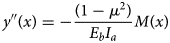
where μ is the Poisson ratio of 0.4 (Wild and others, Reference Wild, Marsh and Rack2017), E b is the elastic modulus of ice 2.7 GPa (Holdsworth and Glynn, Reference Holdsworth and Glynn1981), I a is the moment of inertia and M(x) is the bending moment. Both μ and E b values are based on literature, but matched to our observations. I a and M(x) are computed as follows:
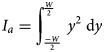
and,
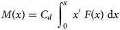
where W is the total mechanically effective width of the ice tongue defined by parallel flowlines derived from surface velocity values, x′ is the relative position along the ice tongue, and C d is the pressure drag coefficient, 1.9 as in (Holdsworth and Glynn, Reference Holdsworth and Glynn1981). Where the force F(x) applied by the sea in the horizontal direction equals the momentum lost per second by the current (Thomas, Reference Thomas1973) equals to,
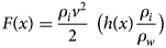
where h(x) is the thickness as a function of the distance, ρ w the water density (1028 kg m−3), v is the tidal current velocity. Following (Holdsworth and Glynn, Reference Holdsworth and Glynn1981), the thickness derived from BedMachine Version 2 (Morlighem, Reference Morlighem2020) was approximated to a linear fit (Fig. S1) using:

The horizontal bending was calculated over the expected mechanical effective proportion of the ice tongue delimited by the derived flowlines shown in the supplementary Figs. 1 and S4. The effective mechanical width from flowlines was based on average surface velocity fields from February 2017 to February 2022. The individual velocity fields were obtained from the on-demand ASF data service (Hogenson and others, Reference Hogenson2020) and post-processed locally. During the post-processing, a smoothing filter was applied, and the images were stacked and averaged.
4. Results
4.1. Fast ice area over McMurdo Sound and Erebus Bay during the study period
Using the fast ice area automatic delimitation approach described in the methods, a time series of fast ice area over the McMurdo Sound was obtained (Fig. 4). An area of influence around the ice tongue was defined to compare the ice tongue dynamics with fast ice changes in the bay, following Gomez–Fell and others (Reference Gomez–Fell, Rack, Purdie and Marsh2022). Using three times the length of the ice tongue from its base, the fast ice area in front of the ice tongue and the embayment is well represented. The area spans Erebus Bay between Hut Point Peninsula to the south, the Delbridge Islands to the north and the northwestern flank of Ross Island to the east (white dashed square in Figs. 1 and 2). The ocean inside the square has a total area of 716 km2. The fast ice area inside the defined area fluctuated from 10.4 to 631.7 km2, with a mean of 376.2 km2 and a standard deviation of 207.9 km2. During the summer of 2018, there was a considerable area of fast ice attached to the ice tongue, while in 2019, there was a long period without fast ice, with repeated breakouts of newly forming ice. According to Leonard and others (Reference Leonard, Turner, Richter, Whittaker and Smith2021), 2019 was a year with rather unusual fast ice cover in the McMurdo Sound.
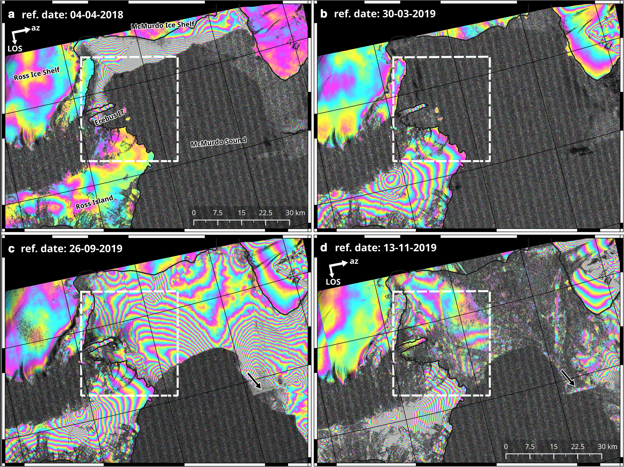
Figure 2. DInSAR images of McMurdo Sound at different stages of fast ice formation. (a) fringes over fast ice that survived the summer, (b) The sound without fast ice at the end of summer, (c) maximum extension of fast ice during winter, and (d) fast ice at maximum extension during spring starting to lose coherence due to surface changes. In panels a) and (d), the flight path (az) and line of sight (LOS) are shown. The black arrow in panels (c) and (d) signals the grounded sliver iceberg that calved from the McMurdo Ice Shelf in March 2016. All the images are in polar stereographic projection.
Fast ice covered the defined area adjacent to the ice tongue during most of the study period. However, natural break-outs occurred during the summer months (January and February), with fast ice regrowth from April onwards. During the summers of 2017 and 2019, the fast ice around the ice tongue retreated almost completely (Figs. 1 and 2b), while in 2018, the fast ice around the ice tongue survived the summer (Figs. 1 and 2a). The maximum extent of fast ice during each of the three years was similar, creating a semi-circumference from Cape Royds to the slither iceberg grounded on the western side of the Sound (Figs. 1, 2c and 2d). Because of the high phase coherence over the fast ice, its formation and evolution over the year can also be observed with interferometric fringes (Fig. 2). The pattern evolution of the fringes varies from the beginning of the winter to the end of spring and from year to year. Sharp changes in the fringe pattern would indicate cracks, ridges or seams that separate areas with independent deformation modes (Dammann and others, Reference Dammann, Eicken, Meyer and Mahoney2016).
4.2. Erebus Ice Tongue InSAR horizontal displacement
InSAR is a precise method to remotely detect displacements at millimetre accuracy at the Earth surface in line of sight of the radar. The one-dimensional nature of the measurement requires additional assumptions for a full interpretation of the displacement. Here, a thorough analysis of an InSAR time series and reasoning for the later differential InSAR (DInSAR) application is presented.
Figure 3 (a to d) shows examples of the interferometric fringe pattern observed over Erebus Ice Tongue in radar imaging geometry. In Figs. 3a,b,d, the ice tongue is embedded in fast ice, while in Fig. 3c, during the summer months of 2019, the fast ice receded completely. A simple fringe count over Erebus Ice Tongue in the azimuth direction seaward of the hydrostatic line (HL) illustrates the large variability in ice displacement in LOS (lateral) over the study period. The fringe counting method is used as a qualitative approach to determine the lateral displacement of the ice tongue and its relation with the fast ice area over time.
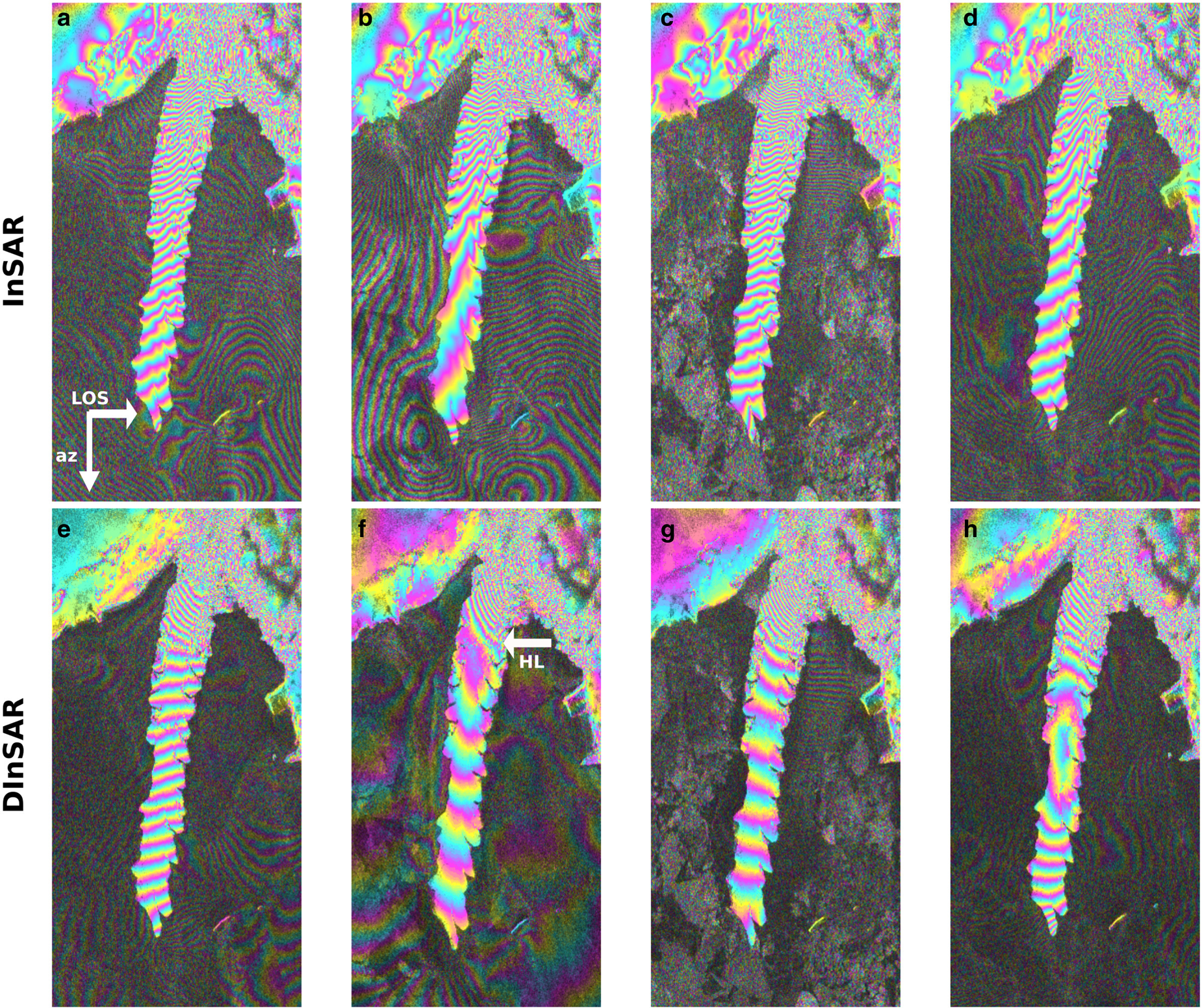
Figure 3. Examples of InSAR and DInSAR fringe patterns over the 10 km long Erebus Ice Tongue from Copernicus Sentinel-1 data. The images are in radar geometry, with range and azimuth directions displayed as white arrows on image (a). (a), (b), (c) and (d) show interferograms with the reference and repeat pass dates as follows: (a) 08-06-2017 and 20-06-2017, (b) 14-09-2019 and 26-09-2019, (c) 30-03-2019 and 11-04-2019 and (d) 14-07-2017 and 26-07-2017. Meanwhile, (e), (f), (g) and (h) images are examples of a complex differential combination of two interferograms. The DInSAR dates are (e) 08-06-2017, 20-06-2017 and 02-07-2017, (f) 14-09-2019, 26-09-2019 and 08-10-2019, (g) 30-3-2019, 11-04-2019 and 23-04-2019, and (h) 14-07-2017 and 26-07-2017 and 07-08-2017. The hydrostatic line (HL) can be seen on all the differential interferograms as a change in the frequency of the fringe pattern and is pointed by a white arrow in panel F.
The analysis of the InSAR fringes time series implies that there is a preferential lateral displacement away (positive) from the sensor (Fig. 4a). When taking into account the sign of the phase difference, the lateral displacement varies strongly and is in 94% of the cases away from the sensor (to the right in Fig. 3). This implies that the ice tongue displacement is variable but consistent in one direction, namely to the north. This persistent displacement towards the north was related to the ice tongue curvature and the component of the ice flow that is in the LOS of the radar. The bias related to the constant flow velocity can be removed when interferograms are differentiated.
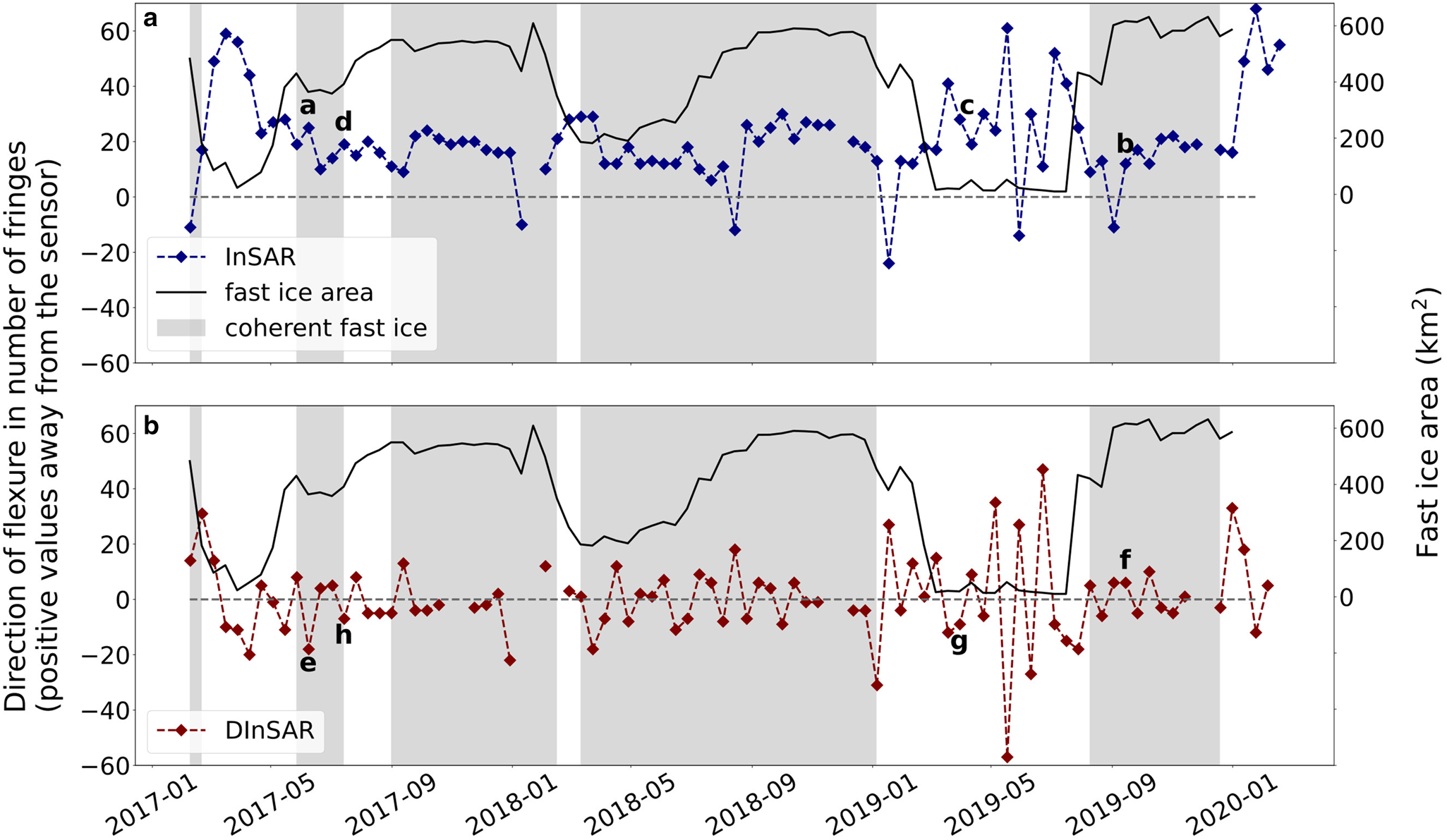
Figure 4. (a) Erebus Ice Tongue direction of flexure from InSAR fringe count time series in blue and fast ice area according to the km2 inside the white dash square in Fig. 2. Letters a, b, c and d represent the reference date of the interferograms shown in 3. (b) Erebus Ice Tongue direction of flexure from DInSAR fringe time series in red and fast ice area according to the km2 inside the white dash square in Fig. 2. Letters e, f, g and h represent the reference date of the differential interferograms shown in 3. The grey shaded area in both graphs represents the periods of time when fringes are visible over the fast ice, which can deviate from the fast ice area due to loss of interferometric coherence between acquisitions. Fringes are counted from the hinge line to the tip of the ice tongue. Positive fringe values indicate displacement away from the sensor, and negative values indicate displacement towards the sensor.
Before doing the differentiation the assumption of constant velocity can be tested and compared to an independent velocity data set. If the assumption is made that displacement occurs completely in the horizontal plane, the fringe count of the InSAR images can be used as a qualitative estimation of horizontal velocity in LOS using the equation for pure horizontal displacement (Rott, Reference Rott2009):

The InSAR fringes can be converted into metres to estimate the mean displacement at the tip of the tongue; if the temporal frame between acquisitions is added, the ice velocity can be estimated. Using the following parameters of the Sentinel-1 sensor on Eq. (6), the C band wavelength (λ) of 5.546 cm, and the IW2 swath nominal incidence angle (θ) at the centre of 38.3$^\circ$ we can convert the fringes over 93 InSAR images of Erebus Ice Tongue to displacement values. When the results are averaged, a mean displacement rate of 30.8 ± 17.9 m yr−1 is obtained. The InSAR velocity is then compared with the average ice surface velocity component in radar LOS from SAR feature tracking is 25.5 ± 8.8 m yr−1 extracted at the tip of the tongue. Both values are in the same order of magnitude, but the feature tracking velocities are slightly lower; we can assume that the difference is the displacement component caused by the currents. Therefore, the following DInSAR Analysis is based on the assumption that there is a constant horizontal flow in the LOS between acquisitions and that when applying differential interferometry, the constant value of the horizontal displacement becomes zero.
4.3. Ice tongue tidal current forcing observed by DInSAR
In this section, the combination of complex interferograms is used to explore the effect of ocean currents over Erebus Ice Tongue. For that purpose, a DInSAR time series is created and analysed. Afterwards, the results are compared with changes in fast ice cover. Lastly, the correlation between the horizontal lateral flexure of the ice tongue and external forces, specifically tidal currents, is explored.
Each consecutive pair of interferograms was combined, generating 92 differential interferograms (DInSAR). This approach aimed to remove the component of constant horizontal ice flow that the sensor can detect, allowing for the isolation of vertical displacements near the grounding line (Rack and others, Reference Rack, King, Marsh, Wild and Floricioiu2017; Wild and others, Reference Wild, Marsh and Rack2019) that defines the flexure zone of the ice tongue and the hydrostatic equilibrium line (Fig. 3f), and for highlighting other deformations (e.g. lateral flexure) (Legrésy and others, Reference Legrésy, Wendt, Tabacco, Rémy and Dietrich2004). Fig. 3 shows four examples of InSAR and four of DInSAR fringe patterns over Erebus Ice Tongue. The differential interferograms over the ice tongue were unwrapped, the displacement values from the centre line A-A’ (inset Fig. 1) were extracted, the values were referenced to a zero start value point, corrected for jumps or errors in the unwrapping results and lastly a Savitzky–Golay smoothing filter was applied.
In Fig. 3 (e to h), examples of the DInSAR results with different fringe patterns and fast ice conditions are shown. The same reference dates for the InSAR and DInSAR images are used. The DInSAR images clearly show the area of the ice tongue subjected to vertical flexure with the hydrostatic boundary signalled by a white arrow in Fig. 3f. The differential displacement of the ice tongue between two InSAR images or the combination of three consecutive acquisitions shows a different pattern than the InSAR images. The DInSAR fringe pattern direction is not constant, observing a reversed pattern in 47% of the images. This means that the ice tongue differential displacement half the time is away from the sensor and the other half towards the sensor, implying that the ice tongue has a back-and-forward differential displacement.
Different fringe patterns were observed when the ice tongue was embedded in fast ice. The DInSAR fringe pattern direction is not constant, observing a reversed pattern in 47% of the images. This means that the ice tongue differential displacement half the time is away from the sensor and the other half towards the sensor, implying that the ice tongue has a back-and-forward differential displacement.
There was a tendency towards fewer fringes when fast ice was present (Fig. 4b). In some cases, the fringes of the ice tongue connect with the fringes over the fast ice, implying the fast ice is mechanically connected to the ice tongue. Grey shaded areas in the graph (Figs. 4a,b) mark when visible interferometric fringe patterns are found around the ice tongue. Loss of coherence occurred in 9% of the DInSAR images. When unwrapping the DInSAR images, the differential displacement spanned from 0 to 1.42 m (Fig. 5). The differential displacement was higher when fast ice was minimal around the ice tongue. When fast ice was minimal or absent, the absolute mean differential displacement was 0.42 ± 0.35 m, and when fast ice was present, the values were 0.18 ± 0.18 m. These values show that fast ice dampened the lateral movement of the ice tongue by a factor of 2. The lateral flexure was higher when there was no fast ice, occurring 34.7% of the time, compared to when the fast ice was present. We observed that flexure outliers in the data associated to periods with fast-ice around the tongue (DInSAR dates: 29-12-107, 10-01-2018 and 22-01-2018 / 05-01-2019, 17-01-2018 and 29-01-2018) occur at the beginning of summer and after a channel is created over the fast ice by the icebreaker that supplies the McMurdo Station in Ross Island, most likely removing the mechanical integrity of the fast ice over the sound.
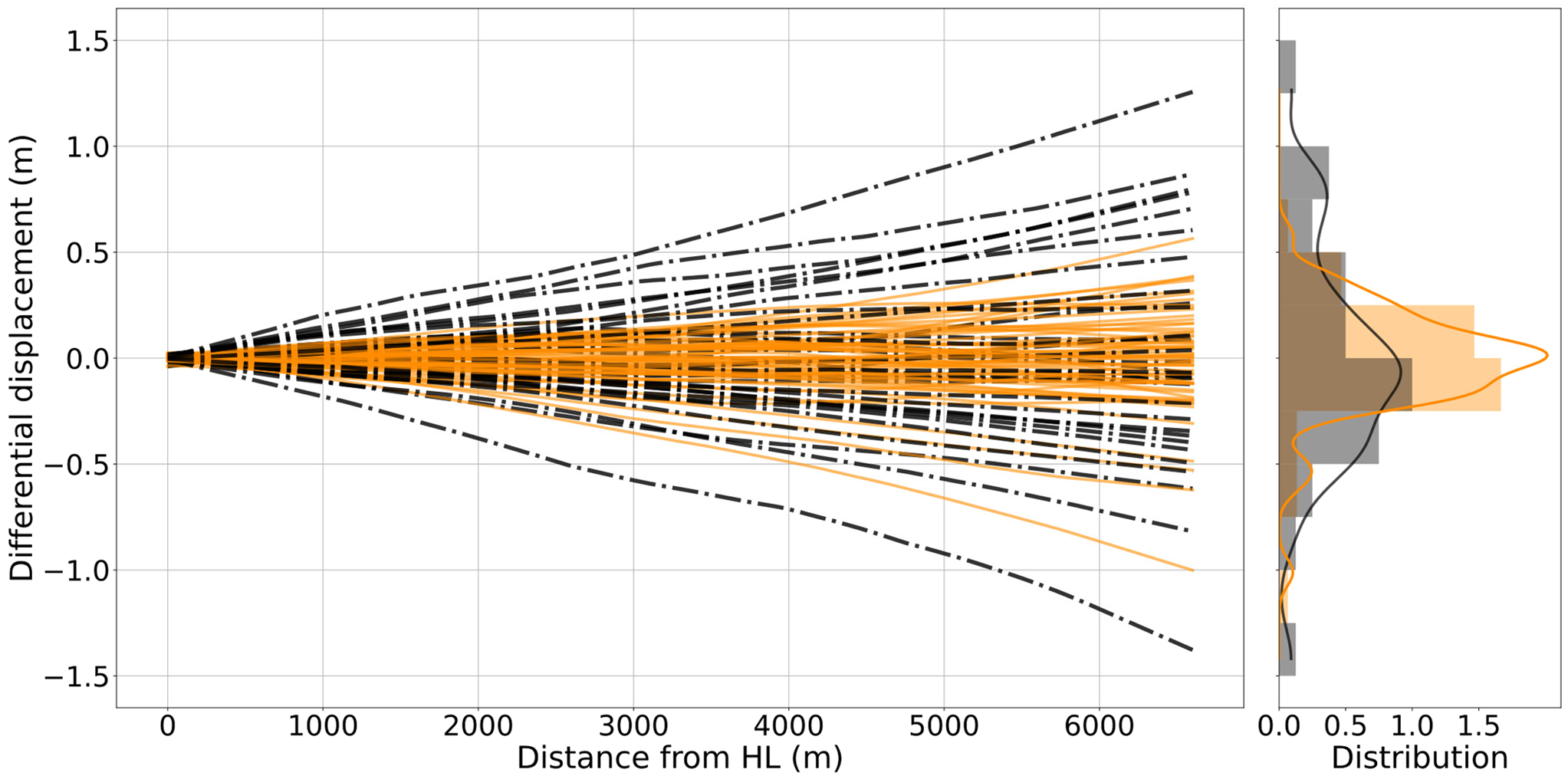
Figure 5. The unwrapped Erebus Ice Tongue DInSAR values over the A--A’ line (Fig. 1) with the probability density function (PDF) at point A’ of each image (plotted on the right). The orange lines are when fast ice is present, and the black dash-dot line represents the DInSAR images when fast ice is absent. The same colour pattern is used for the PDF on the right.
To evaluate if there was a statistical difference between flexure with or without the presence of fast ice, we use the Wilcoxon-Mann-Whitney test (Fay and Proschan, Reference Fay and Proschan2010), and we found that the difference between the samples is significant (p-value of 0.0003). We also looked at the correlation between the presence/absence of fast ice and deformation at the tip of the ice tongue using a Point Biserial Correlation (PBC) (Kornbrot, Reference Kornbrot, Everitt and Howel2014). We obtained a moderate but significant correlation (0.40 with p-value 0.00006) between the absence of ice and the flexure.
4.4. Correlation between displacement and tidal currents
Tidal currents values obtained from the CATS2008 tide model 12, 8, 6, 4, 2 and 1 hour before each SAR image acquisition were integrated. Each ocean current integration was compared to the tidal current values of each DInSAR displacement. Tidal current values were differentiated twice to produce a differential current between three consecutive dates, comparable with a differential displacement of three consecutive SAR images. The best correlation values between differential currents and the differential displacement were using tide data from 1 and 2 hours before the acquisition.
Tidal currents orthogonal to the ice tongue correlate well with the ice tongue displacements when the direction is considered, and fast ice is absent. When comparing differential displacements at periods without fast ice (Figs. 4 and 5) with differential currents values, a Pearson correlation of 0.45 (p-value 0.009) and 0.45 (p-value 0.008) for 1 and 2 hours before image acquisition is obtained, respectively. When fast ice was present, the correlation was low, 0.27 (p-value 0.01) and 0.25 (p-value 0.02) for 1 and 2 hours prior to image acquisition, respectively. This highlights the effect of fast ice over the ice tongue and how it reduces its flexure. Fig. S5 shows a scatter plot of the relation between DInSAR displacement in fringes compared to the differential tidal currents from the CATS2008 tidal model orthogonal to the ice tongue when fast ice is absent (R-squared of 0.23 and a p-value of 0.0079).
Moreover, when doing a Pearson correlation between fast ice extent, InSAR and DInSAR and the number of fringes, a -0.50 (p-value 4.9 e--07) for InSAR and -0.32 (p-value 0.003) for DInSAR fringes with fast ice extent in km2 is obtained. The negative relation of the relationship indicates that when fast ice is absent, the horizontal displacements in LOS over the ice tongue are larger.
4.5. Analysis of Erebus Ice Tongue mechanics
The analysis of the elastic model results provided an observational-based framework for estimating the forces exerted by ocean currents over the ice tongue (Fig. 6b). The steady-state creep bending stresses assume that the expected currents are not entirely tidal-based, but that the background current (Stevens and others, Reference Stevens, Stewart, Robinson, Williams and Haskell2011, Reference Stevens2014; Leonard and others, Reference Leonard2006) results in a significant component of the overall pressure exerted by the ocean on the ice tongue. Assuming that the pressure of the background ocean current is constant, we can calculate the effective maximum bending stress on the ice tongue (Fig. 6c) using the following equation Holdsworth (Reference Holdsworth1982):
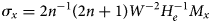
where σ x is the maximum bending stress, n the creep exponent is taken as 3, W the effective mechanical width, M x the moment at a distance x from the GL, and H e is the considered effective thickness. H e is calculated as 0.75 H(x) the estimated value at the edges according to Holdsworth (Reference Holdsworth1982). Using equation (7) it was found that the most likely stresses are between 0.3 and 0.45 1 × 10⁵ N m −2 (Fig. 6c).
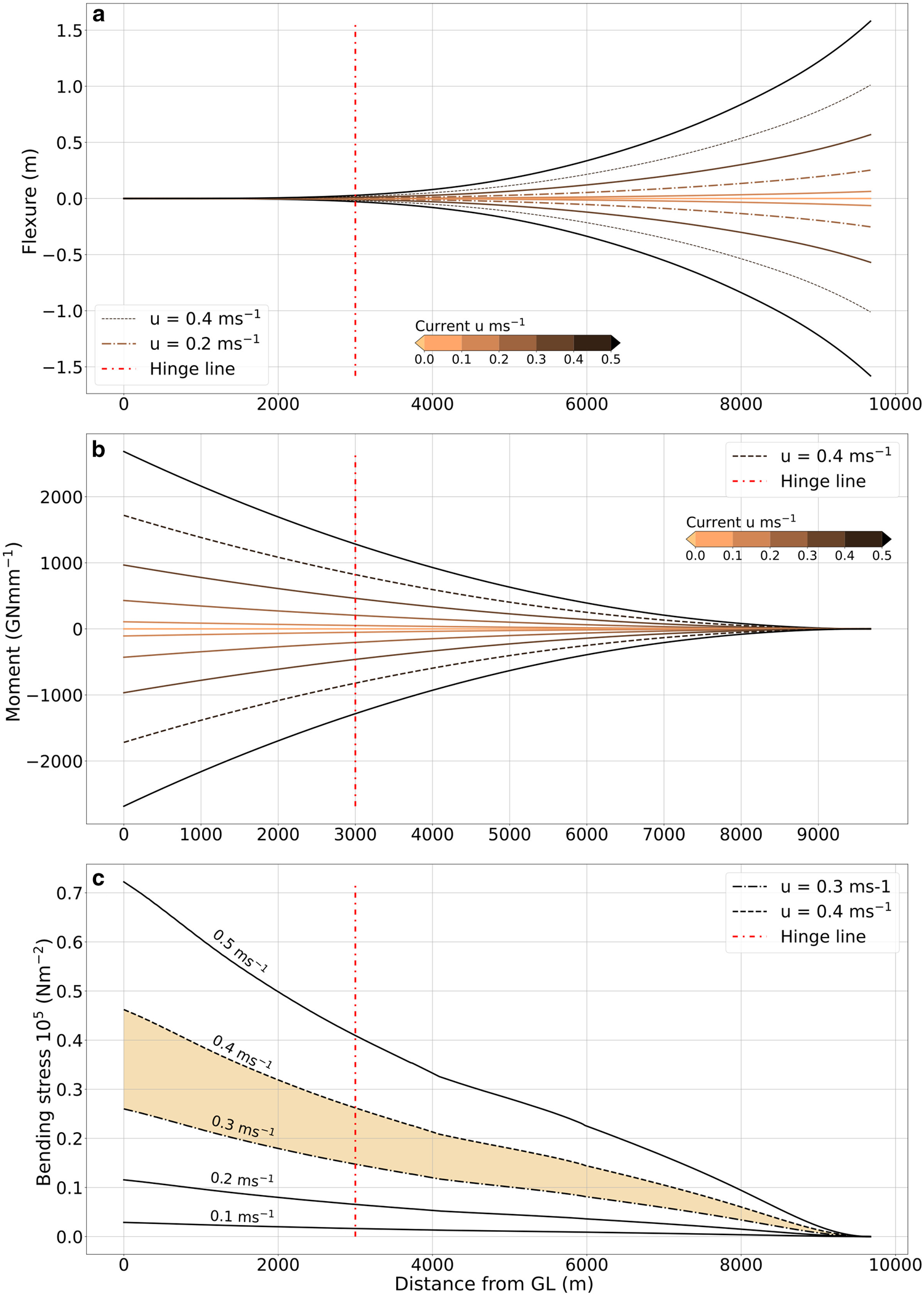
Figure 6. (a) Analytical model of flexure from the GL to the tip at tidal currents ranging from -0.5 to 0.5 m s−1 at every 0.1 steps, using E b ± 2.7 GPa (Holdsworth and Glynn, Reference Holdsworth and Glynn1981) and a drag coefficient (C d ) of 1.3. (b) Moment of bending from the GL to the tip at currents between -0.5 to 0.5 m s−1. (c) Stresses derived from equation (7) are plotted. The orange area illustrates where the highest stresses generated by tidal currents over the ice tongue are most likely to occur. The red dot-dashed line marks the DInSAR hydrostatic line.
From the model, it was found that current velocities in the range of -0.45 to 0.3 m s−1 (sign denotes direction) aligned well with the observed differential flexure (Fig. 5). These results align with observed velocities in the vicinity of the ice tongue (Leonard and others, Reference Leonard2006; Stevens and others, Reference Stevens, Stewart, Robinson, Williams and Haskell2011, Reference Stevens2014). On the contrary, perpendicular current velocities derived from the tide model are lower than the ones used in the model to match the observations. This probably mean that the tidal model is not resolving the complexity of the current patterns in the vicinity of Erebus Ice Tongue. From the stresses calculated (0.25 × 10⁵ N m −2 at a current value of 0.3 m s−1 and 0.46 × 10⁵ N m −2 at a current value of 0.4 m s−1), it seems that the bending of the ice tongue forced by the tidal currents is, at this point, not enough to generate failure (Fig. 6c), as ice will fail with stress values higher than 1 × 10⁵ N m −2 (Cuffey and Paterson, Reference Cuffey and Paterson2010) and the most likely higher stresses lay in the orange filled polygon in Fig. 6c.
4.5.1. E b and C d sensitivity analysis
Holdsworth and Glynn (Reference Holdsworth and Glynn1981) modeled Erebus Ice Tongue bending moment and stress. The ice tongue at that time had a total length of 12750 m. They assume a linear relation between thickness and distance from the grounding line and an ocean current velocity of 0.5 m s−1, obtaining a total moment distribution considering the complete ice tongue on the same order of magnitude as the results presented here. As expected, using the same value for current and flexure, the total displacement, momentum, and stress of the tongue are in good agreement with Holdsworth (Reference Holdsworth1982). The values obtained by Holdsworth (Reference Holdsworth1982) are slightly higher than the observations presented in the analytical model section. Using the analytical model, a sensitivity analysis was conducted over the flexure derivation to constrain the values that fit the DInSAR observations.
In Fig. 6a, the modelled bending pattern from the HL can be observed. An elastic modulus (E b) of 2.7 GPa was used in accordance with (Holdsworth and Glynn, Reference Holdsworth and Glynn1981). More recent measurements in the vicinity of the McMurdo Ice Shelf place the E b value closer to 1.6 GPa (Wild and others, Reference Wild, Marsh and Rack2017). To try to pinpoint a range of probable values for E b over Erebus Ice Tongue, a sensitivity analysis was performed (Fig. 7a). For the model formulation, a higher-end current value of 0.4 m s−1 is used in accordance with values derived in the analytical model section.
Figure 7. Sensitivity analysis of the flexure for (a) the elastic modulus (E b in GPa) and (b) the drag coefficient (C d) at a fixed current velocity value of 0.4 m s−1. The area between the dashed and dotted dashed lines mark the most probable lateral bending at 0.4 m s−1 .
The results of the E b sensitivity analysis (Fig. 7a) show that the possible values of E b according to the observed maximum differential displacement of the tongue at the higher end of the current velocities are between 1.4 and 1.8 GPa (between the dashed line and dashed dot line in Fig. 7a). This is similar to the 1.6 GPa value for E b found in the nearby McMurdo Ice Shelf by Wild and others (Reference Wild, Marsh and Rack2017).
A sensitivity analysis over the pressure drag coefficient was also performed (Fig. 7b). The drag coefficient has two components, one related to the shape of the obstacle and the other related to the roughness at the boundary. Because an ice tongue is a barrier to the surface currents (Stevens and others, Reference Stevens2017) we use the shape drag as the input in equation (3). Drag coefficients depend on the Reynolds number and are normally defined by empirical methods. Here the assumption of turbulent flow is used. The range of values of the pressure drag coefficients from a smooth ball (0.1) to a perpendicular Long flat plate (1.9) perpendicular to a turbulent flow are explored. The values that better represented the drag coefficient for Erebus Ice Tongue are between 1.1 and 1.5 (between the dashed line and dashed dot line in Fig. 7b). Holdsworth and Glynn (Reference Holdsworth and Glynn1981) used 1.95 as a value for the drag coefficient in their formulation. This value should not be mistaken for the skin drag coefficient used in turbulent fluxes for melt rate calculations (Rosevear and others, Reference Rosevear, Galton-Fenzi and Stevens2022). A plot of the flexure in relation to changes in the drag coefficient (C d) and the Elastic Modulus (E b) is shown in the supplementary materials (Fig. S6).
5. Discussion
The observations presented here show that fast ice hinders lateral flexure and can mechanically connect with the ice tongue, diminishing the forcing of lateral currents. This has been suggested by Holdsworth and Glynn (Reference Holdsworth and Glynn1981), and partially observed by Legrésy and others (Reference Legrésy, Wendt, Tabacco, Rémy and Dietrich2004) by using four one-day interferograms and Global Positioning System (GPS) measurements but without taking fast ice processes into account. Here a three-year continuous time series of interferograms (93 in total) is presented jointly with a fast ice time series. This allows for the observation of the flexure of the ice tongue and its evolution during the year. We observe that ice tongues can present substantially higher amplitudes of lateral displacement when fast ice is absent. This supports the theory that fast ice can stabilise ice tongues and potentially supress fracturing (Gomez–Fell and others, Reference Gomez–Fell, Rack, Purdie and Marsh2022). Various mechanisms can trigger calving events on ice tongues (e.g. Holdsworth, Reference Holdsworth1985; Massom and others, Reference Massom2015). Stresses generated by lateral bending of the ice tongue enhanced by ocean currents or swell are among them (Stevens and others, Reference Stevens, Sirguey, Leonard and Haskell2013). Holdsworth (Reference Holdsworth1982) states that for a calving event to happen, several mechanisms must work together to trigger an event. Holdsworth and Glynn (Reference Holdsworth and Glynn1981) speculated that some of these mechanisms are triggered by swell-induced oscillations.
Erebus Ice Tongue has calved four times in recorded history (1911, 1942, 1990 and 2013) (Stevens and others, Reference Stevens, Sirguey, Leonard and Haskell2013). The two latest calving events, which have been studied in more detail (Robinson and Haskell, Reference Robinson and Haskell1990; Stevens and others, Reference Stevens, Sirguey, Leonard and Haskell2013), have one observation in common: there was no fast ice present around the ice tongue at the time of calving. Robinson and Haskell (Reference Robinson and Haskell1990) speculate that storm swells created a lateral force that pushed against the side of the ice tongue, initiating the calving. Stevens and others (Reference Stevens, Sirguey, Leonard and Haskell2013) suggests that by crossing at the longitude of Tent Island, the ice tongue is more exposed to ocean forcing, getting caught between a main northward current and a returning current from the south, generating current shear. In both cases, the calving of Erebus Ice Tongue involves lateral flexure of the tongue by shear currents or storm swell at a period where fast ice is absent.
Research about the effect of currents or tidal currents over ice tongues is sparse in time and space. Holdsworth (Reference Holdsworth1969) formulated the possibility of finding the lateral movement of ice tongues. Thomas (Reference Thomas1973) compared the relation with an elastic beam fixed at one end and solved it, and Holdsworth (Reference Holdsworth1982) modelled the relation using data from Erebus Ice Tongue. Legrésy and others (Reference Legrésy, Wendt, Tabacco, Rémy and Dietrich2004) gave the first observation of the phenomena using GPS and remote sensing from SAR over the Mertz Ice Tongue. Our three-year time series of InSAR and DInSAR measurements validate previous observations and expand its knowledge with information about seasonal changes and their interaction with fast ice presence.
We found that the formation of fast ice around the ice tongue subdues horizontal oscillations (Fig. 5). Because lateral flexure can cause the onset of fracture, our observations show that fast ice can be a protective mechanism that prevents mechanical failure. The mechanism that prevents failure is not completely clear as the fast ice is at least an order of magnitude thinner than the ice tongue and could not exert enough pressure to resist the ice tongue dynamics. The mechanical coupling between the ice tongue and the fast ice, as shown in the interferometric images, most likely strengthens the ice tongue's mechanical integrity. The fact that the ice tongue is in the middle of Erebus Bay and that the fast ice during winter creates an embayment is of interest. The fast ice creates a continuity between Erebus Ice Tongue, the land and the Dellbridge Islands. It would be interesting to observe if this is the case with other ice tongues that do not form these types of embayments when connected with fast ice during the winter months (e.g. Nordenskjold Ice Tongue).
Erebus Ice Tongue has a well-known bend towards the north (e.g. Holdsworth, Reference Holdsworth1982; Stevens and others, Reference Stevens, Sirguey, Leonard and Haskell2013). The speculation has been that this bend is due to a northwest recirculation of the main current that enters the eastern McMurdo Sound from the north (Holdsworth, Reference Holdsworth1982; Leonard and others, Reference Leonard2006; Stevens and others, Reference Stevens2014). Our findings support this theory as observations show a constant displacement of the ice tongue to the north in the interferometric results. This is most likely due to a recirculation current that pushes the ice tongue almost all year round. When variable tidal currents are added to this background current, an oscillatory effect appears on the DInSAR results (Video S1). The lateral oscillation observations can be replicated with a simple analytical model, using some assumptions based on literature about the local currents (Stevens and others, Reference Stevens, Stewart, Robinson, Williams and Haskell2011, Reference Stevens2014; Leonard and others, Reference Leonard2006). These lateral oscillations, in combination with other factors, could help the onset of ice tongue fracture and calving (Holdsworth and Glynn, Reference Holdsworth and Glynn1981).
Observations of ocean currents in the vicinity of Erebus Ice Tongue (Stevens and others, Reference Stevens, Stewart, Robinson, Williams and Haskell2011, Reference Stevens2014) and Erebus Bay (Leonard and others, Reference Leonard2006) have shown near-surface maximum current values between 0.3 to 0.4 m s−1, with typical values around 0.15 to 0.2 m s−1 (Stevens and others, Reference Stevens, Stewart, Robinson, Williams and Haskell2011). These current values match the lateral flexure observations shown here when applied to the flexure analytical model. Holdsworth (Reference Holdsworth1982) and Holdsworth and Glynn (Reference Holdsworth and Glynn1981), when modelling the bending pattern of the tongue, used a current velocity of 0.5 m s−1, regarded as conservative at the time of the study. According to the same work, current alone does not excert the amount of stress sufficient to break up the ice tongue. This is corroborated by our observations that show that the lateral bending of the tongue and the related current values generate maximum stresses between 0.3 and 0.45 × 10⁵ N m −2, below the 1 × 10⁵ N m −2 threshold that would initiate mechanical fracture (Cuffey and Paterson, Reference Cuffey and Paterson2010). Nonetheless, fracture might occur if stresses from lateral bending are combined with creep stresses and stresses from strong oscillations like storm swell or tsunamis (Holdsworth and Glynn, Reference Holdsworth and Glynn1981; Brunt and others, Reference Brunt, Okal and MacAyeal2011). The complete calving of the Parker Ice Tongue in 2020 was probably generated by a sum of these stresses and facilitated by the absence of fast ice that generated additional support (Gomez–Fell and others, Reference Gomez–Fell, Rack, Purdie and Marsh2022).
It is worth noting that the stresses were calculated assuming viscous creep rather than elastic deformation. On shorter time scales, stresses might be balanced by elastic deformation rather than viscous creep. This difference between quasi-instantaneous and long-term deformation partly explains the difference between observations and the model. Our measurements are discontinuous and at a different time scale than tides; we tried to solve this problem by differentiating the value of the integrated tidal current before each satellite acquisition. Combining continuous deformation measurements of in situ flexure with concurrent observation of ocean currents would help overcome the time scale difference between tidal forces and deformation observed by satellite images.
The present Victoria Land Coast icescape has the ideal conditions for the formation of ice tongues. Hall and others (Reference Hall2023) show that this has not always been the case. In the past, ice tongues were probably absent in the region due to higher air and oceanic temperatures and different fast ice distribution (Hall and others, Reference Hall2023). This indicates that future changes in ocean temperature will most likely affect ice tongue mass balance and fast ice extent, which in turn will affect the stability of ice tongues in the region.
6. Conclusions
This article presents a three-year time series of interferogram observations over Erebus Ice Tongue. The results showed that ocean currents induced the lateral flexure of the ice tongue and that this bending was more pronounced when fast ice was absent. The results support previous interpretations for Erebus Ice Tongue's lateral bending while better constraining the flexure. The observations also match the estimated currents in the area and the effect of the ice tongue lateral flexure on the iceF flow. The results implied a significant correlation (0.45) between the ice tongue lateral flexure and tidal currents when fast ice was absent.
On the other hand, when fast ice surrounds the ice tongue, the correlation between lateral flexure and tidal currents is insignificant. Moreover, the absolute average displacement at the tip of the tongue was 0.44 ± 0.37 m when fast ice was absent, and 0.19 ± 0.18 m when fast ice was present. This shows that fast ice hinders the lateral movement of the ice tongue related to tidal currents, reducing the overall stresses. Mechanical fracture occurs when a combination of stresses from different sources surpasses the yield stress. Ocean currents in the vicinity of Erebus Ice Tongue, on their own, are likely too small to produce stresses that result in a complete break-off. Nonetheless, this work highlights the importance of fast ice as a mechanical strengthening of ice tongues, and it poses the question of how ice tongue stability will be impacted if fast ice around Antarctica starts declining in the future.
Supplementary material
The supplementary material for this article can be found at https://doi.org/10.1017/jog.2024.21
Acknowledgements
RG acknowledges the support of the University of Canterbury and the Antarctic New Zealand Sir Robin Irvine Doctoral Scholarships. The New Zealand Antarctic Science Platform and the Antarctic and High Latitude Climate Project partially funded WR. Copernicus Sentinel data from 2017, 2018, 2019 and 2020 were retrieved from ASF DAAC in August 2021 and processed by ESA. Velocity data was generated using auto-RIFT (Lei and others, Reference Lei, Gardner and Agram2021) and provided by the ASF Vertex platform, using HyP3 (Hogenson and others, Reference Hogenson2020). We thank the scientific editor (M. Siegfried) and the reviewers (T. Wagner and one anonymous reviewer) for their time, expertise, and valuable feedback that improved the quality of this manuscript.


 Open access