


1. Introduction
It is widely accepted that ice sheets behave like an incompressible non-Newtonian fluid, modeled by the Stokes equations with nonlinear rheology (Reference BengtssonBengtsson, 1994; Reference Gregory and HuybrechtsGregory and Huybrechts, 2006; Reference Cuffey and PatersonCuffey and Paterson, 2010). Due to the high computational costs associated with the solution of the Stokes equations over large, three-dimensional (3-D) domains, such as Greenland or Antarctica, several approximations have been considered (Reference HindmarshHindmarsh, 2004). These approximations exploit the fact that the aspect ratio, 5, between the characteristic thickness and the characteristic horizontal extent of an ice sheet is very small. In increasing order of accuracy of the solution with respect to δ, we have the zeroth-order (ZO) models, such as the shallow-ice approximation (SIA; Reference HutterHutter, 1983) and the shallow-shelf approximation (Reference Morland, Van der Veen and OerlemansMorland, 1987; Reference MacAyealMacAyeal, 1989), and higher-order models, such as the depth-integrated L1L1 and L1L2 models (Reference HindmarshHindmarsh, 2004) and the 3-D Blatter-Pattyn model (Reference BlatterBlatter, 1995; Reference PattynPattyn, 2003), hereafter referred to as the first-order (FO) model.
Higher-order models can be regarded as a trade-off between accuracy and computational costs. In this work, we consider the FO model presented by Reference Dukowicz, Price and LipscombDukowicz and others (2010), which is based on the Blatter-Pattyn model (Reference BlatterBlatter, 1995; Reference PattynPattyn, 2003) and the modified version of the L1L2 model of Reference Schoof and HindmarshSchoof and Hindmarsh (2010). The resulting mathematical models consist of a system of two nonlinear elliptic equations for the horizontal velocities. The FO model is a fully 3-D model, whereas the L1L2 is depth-integrated and reduces to a two-dimensional (2-D) elliptic system in the horizontal coordinates. Reference Dukowicz, Price and LipscombDukowicz and others (2010) and Reference Schoof and HindmarshSchoof and Hindmarsh (2010), respectively, show that there exist variational principles associated with both the FO and the L1L2 models. In fact, the two problems are equivalent to the unconstrained minimization of associated positive functionals. In contrast, the Stokes model is equivalent to a constrained minimization problem (Reference Dukowicz, Price and LipscombDukowicz and others, 2010) in which the pressure plays the role of a Lagrange multiplier. Therefore, besides the reduction in the number of variables (from four to two), the higher-order models have mathematical properties which are more favorable than the Stokes model from a numerical point of view. Moreover, the L1 L2 model has the clear advantage of being a 2-D model.
In this work, we propose a finite-element (FE) approximation of the higher-order models at hand. Using finite elements, complex geometries and unstructured and anisotropic meshes can be naturally handled, as can several physical boundary conditions. Moreover, finite elements are particularly suited for the solution of the problems at hand. In fact, when the bilinear form associated with the weak formulation of the linearized problem is symmetric and coercive, as in the case of the considered higher-order models, Galerkin FE methods become projection methods (Reference Bochev and GunzburgerBochev and Gunzburger, 2009). This means that the computed solution is the ‘best’ approximation to the exact model solution among all possible functions in the chosen FE space.
We implement the higher-order models using the C++ FE library LifeV (www.lifev.org). We compare our implementation against tests A, C and E of the ISMIP-HOM benchmark experiments (Reference PattynPattyn and others, 2008). In particular, we compare our results with the reference Stokes solutions provided by Reference Gagliardini and ZwingerGagliardini and Zwinger (2008). We also compare our solutions with those obtained by the higher- order methods presented in the ISMIP-HOM benchmark. It turns out that our FO solutions are in general closer to the reference Stokes solutions than most of the FO solution methods discussed in the ISMIP-HOM benchmark. Also, for medium to small values of the aspect ratio, δ, the proposed L1L2 model presents good agreement with the Stokes solution in the presence of sliding boundary conditions.
In this work, we use both linear (P1) and quadratic (P2) finite elements. Linear elements provide a second-order accurate approximate solution, whereas quadratic elements provide third-order accuracy (in L 2 norm). A comparison between the solutions obtained with linear and quadratic finite elements is carried out for the FO model. As expected, quadratic elements provide better solutions than linear ones, the improvement being more pronounced in the presence of sliding boundary conditions.
The paper is organized as follows. In section 2, we introduce the FO and L1L2 mathematical models including boundary conditions and weak formulations. A brief derivation of the models as an approximation of the Stokes model is also presented. In section 3, we define the FE discretization of the problems at hand. In section 4, we report on the results of the numerical experiments using three ISMIP-HOM benchmark tests. In particular, we compare our L1L2 and FO models against a Stokes model, compare our FO model to other implementations of the FO model and compare our L1 L2 model against other depth-integrated higher-order models. Also we compare the Newton and Picard approaches and the use of structured meshes versus locally refined unstructured meshes. Finally we compare the use of linear and quadratic FE approximations.
2. Mathematical Model
2.1. Stokes model
Ice-sheet flows are typically modeled as non-Newtonian incompressible fluids obeying the Stokes equations. A quasi-static approximation is generally adopted because inertial terms (time derivatives and advective terms) can be neglected, due to the slow movement of the ice. Denoting the ice velocity as u and the Cauchy stress tensor as σ, the Stokes model is given by
where ρ denotes the ice density and g the gravitational acceleration, g ≈ {0,0, – |g|} = {0,0, – g}. The Cauchy stress tensor is given by

Where τ denotes the deviatoric stress tensor, μ the ice effective viscosity, p the ice pressure, l the identity tensor and ![]() the strain-rate tensor defined as
the strain-rate tensor defined as

The effective viscosity, μ, is given by Glen’s law (Reference NyeNye, 1957; Reference Cuffey and PatersonCuffey and Paterson, 2010)
where the effective strain rate, ![]() , and the effective stress, τe, are given by
, and the effective stress, τe, are given by

and where A denotes the flow rate factor which is strongly dependent on the ice temperature.
Stokes boundary conditions
Let the ice domain, Ω, be bounded by the upper surface, Γs, the lower surface, Γb, and the vertical lateral surface, Γl, defined as

We require that Γs ∪ Γb ∪ Γl = ∂Ω, the whole boundary of Ω. The lateral surface, Γl, can be void.
On the upper surface, a stress-free boundary condition is prescribed:
where n is the unit vector normal to the surface and outwardpointing. On the lower surface, we consider no-slip or sliding boundary conditions, i.e. if we partition Γb into Γ0 and Γβ, we have

where β ≥ 0 is the sliding coefficient and the operator (·)|| performs the tangential projection onto the surface.
2.2. First-order model
The FO model is derived as an approximation of the Stokes model under the assumption that the aspect ratio, δ, is small and that the normals to the upper and lower surfaces are almost in the vertical direction, that is, n ~ [O(δ), O(δ), 1]T. Loosely speaking, the FO model is obtained neglecting those terms of the Stokes model that are O(δ 2) (Reference BlatterBlatter, 1995; Reference PattynPattyn, 2003; Reference Dukowicz, Price and LipscombDukowicz and others, 2010).
We denote with u, v and w the components of the velocity along the x, y and z directions, respectively. In the first- order approximation, the terms ∂w/∂x and ∂w/∂y are negligible with respect to ∂u/∂z; hence, ![]() and
and ![]() are approximated as
are approximated as ![]() and
and ![]() , respectively. Exploiting the fact that, due to incompressibility,
, respectively. Exploiting the fact that, due to incompressibility, ![]() , the effective strain rate reduces to
, the effective strain rate reduces to
Moreover, the terms ∂σzx /∂x and ∂σzy/∂y are negligible with respect to ∂σzz /∂z; therefore from the vertical component of the momentum equation (Equation (1)), we have
Integrating this equation along the vertical direction between z and the top surface, s, and prescribing the stress-free boundary condition on that surface, we obtain an expression for the pressure:
Substituting Equation (11) into the horizontal components of the momentum equation (Equation (1)), we obtain the first- order equations

Where

Boundary conditions for the first-order equations
In the FO approximation, the boundary conditions (Equations (7) and (8)) reduce to

These boundary conditions, proposed by Reference Dukowicz, Price and LipscombDukowicz and others (2010), are slightly different from those proposed by Reference PattynPattyn (2003). Reference PattynPattyn (2003) takes the normals, n, as  on Γs, and
  on Γβ, whereas we normalize them to have unit length, i.e. we divide them by
 ![]() and
and ![]() respectively.
respectively.
Weak formulation of the first-order equations
We denote with V the Hilbert space defined as V = [φ ∊ H 1 Ω) : φ |Γ0 = 0}. Here, H 1 (Ω) denotes the space of square- integrable functions whose first derivatives are also square integrable. The weak formulation of Equation (12) reads: find u, v ∊ V such that

for all φ1, φ2 ∊ V(Ω). Whenever periodic boundary conditions are applied on Γl, we require that the functions in V be periodic. (Reference SalsaSalsa, 2008, provides an introduction to Sobolev spaces and weak formulation.)
We define the operator _(u, v; φ 1, φ 2) as the left-hand side of the system given in Equation (15).Then, the problem of Equation (15) is equivalent to finding the root (u, v) ∊ [V]2 of the nonlinear equation
In order to find the roots of Equation (16), we use Newton’s method. Details are given in the Appendix. Newton’s method is an iterative algorithm and requires an initial guess, (u 0, v 0).
It is not possible to take (0, 0) as the initial guess because in this case the effective viscosity, μ, would not be defined. Instead, we compute (u
0, v
0) by solving Equation (15) for a given viscosity, ![]() . (The value of
. (The value of ![]() influences the convergence of the iterative scheme. Here we take
influences the convergence of the iterative scheme. Here we take ![]() which has been determined empirically. If an estimate of the effective strain,
which has been determined empirically. If an estimate of the effective strain, ![]() is available, one can take
is available, one can take ![]()
2.3. L1L2 approximation
The L1L2 model approximates the FO model, retaining almost the same order of accuracy. It requires the solution of 2-D nonlinear partial differential equations. The L1L2 model presented here is derived by Reference Schoof and HindmarshSchoof and Hindmarsh (2010), where it is shown to have the same accuracy as the FO model for fast-sliding regimes. It is devised for sliding boundary conditions and, in the limit case of noslip boundary conditions, it reduces to the zeroth-order SIA model. The model proposed by Reference Schoof and HindmarshSchoof and Hindmarsh (2010) is limited to planar geometries living in the vertical x-z plane. Here we present its natural extension to 3-D geometries.
We define the norm |·||| as
and the norm | · |⊥ as
We also denote with ∇|| the operator ![]()
The effective deviatoric stress reads ![]() For the L1L2 model, we use the SIA (Hutter, 83) to estimate
For the L1L2 model, we use the SIA (Hutter, 83) to estimate ![]()
Hence, we have
We then approximate the horizontal components of ![]() at the bedrock (z = b) with
at the bedrock (z = b) with

Taking the norm | · ||| of both sides of Equation (21), we obtain

where ![]() Equation (22) implicitly defines |τ||| as a function of
Equation (22) implicitly defines |τ||| as a function of ![]() This allows us to solve Equation (21) and determine the horizontal components of τ :
This allows us to solve Equation (21) and determine the horizontal components of τ :
Integrating the first-order Equation (12) from z = b to z = s, and applying the sliding boundary conditions (Equation (14) 1,3) we have

where

and

Solving these equations we obtain the basal velocities, u b(x, y) and v b(x, y).
In order to obtain the velocities, u(x, y, z) and v(x, y, z), we need to compute τ xz and τ yz . Integrating the first-order Equation (12), along the vertical direction, from z, and applying stress-free boundary conditions (Equation (14) 1), we have

where

The effective stress, τe, can be recovered as
The horizontal velocity components, u and v, are obtained by integrating ![]()

Note that Equation (24) are only defined when sliding boundary conditions are prescribed at the bedrock. In the limit case of no-slip boundary conditions, the basal velocity components are known (u b = v b = 0), and the stress terms, τxz and τyz , as well as the velocities, u and v, reduce to the SIA values. In this case, the horizontal velocity components read

Weak formulation of the L1L2 problem
The nonlinear elliptic equations (24) are solved in the 2-D domain, Σ, which is the projection of Ω onto the x- y plane. Typically, stress-free or no-slip boundary conditions are prescribed on δΣ. We denote with Λ0, Λs, Λ1 the portions of δΣ where no-slip, stress-free and periodic boundary conditions are prescribed, respectively. The weak formulation for Equation (24) is similar to the FO one. We define the Hilbert space, V Σ, as V Σ= {φ ∊ H 1(Σ): φ|Λ0 = 0}.The weak formulation of the problem is given by: find u, v ∊ V Σ such that

for all φ1, φ2 ∊ V Σ. When periodic boundary conditions are applied on Λ1, we require that the functions in V Σ be periodic, while stress-free boundary conditions (on Λs) are naturally included in the weak formulation. As in the FO case, we use Newton’s method to solve the problem. Details are given in the Appendix.
3. Numerical Discretization and Implementation
In this section we briefly describe the FE discretization of the weak formulation, Equation (15). (See, e.g., Reference Quarteroni and ValliQuarteroni and Valli, 1994; Reference QuarteroniQuarteroni, 2009, for an introduction to FE methods.) The discretization for the 2-D case, i.e. for the formulation of Equation (32), is not provided here because it can be inferred from the 3-D one. In particular, a triangular mesh is considered instead of a tetrahedral one.
Let Th denote a tetrahedral triangulation of the ice domain, Ω. Here, h is the maximum diameter of the tetrahedral elements in Th . We consider the FE space Pk,h (T h) consisting of continuous functions on Ω whose restriction to any tetrahedron in Th is a polynomial of degree k. We denote with P1 and P2 the FE space associated with P 1,h and P 2, h , respectively. The four (three in 2-D) degrees of freedom (DOF) of P1 elements correspond to values at the vertices of the tetrahedra (triangles in 2-D). The ten (six in 2-D) DOF of P2 elements correspond to values at the vertices of the tetrahedra and at the midpoints of the edges of the tetrahedra (triangles in 2-D). We denote with Vh the finite-dimensional subspace of V defined as Vh = {v h ∊ P k,h : v h |Γ0 = 0} for k = 1 or 2, depending on the finite element chosen. The discretized problem follows from the continuous weak formulation, Equation (15), by replacing V with Vh .
Numerical implementation
The numerical model has been implemented using the C++ parallel FE library ‘LifeV’, which interfaces with ‘Trilinos’ (http://trilinos.sandia.gov) for parallel solvers and data structures. The discrete operators are assembled using different quadrature rules. When using P1 elements, we used a 1-point quadrature rule for assembling the stiffness matrix because in this case the gradients of the basis functions are constant on each element. We used a 15-point (6-point in 2-D), fourth-order accurate quadrature rule in the P2 case. The meshes are partitioned using ‘Parmetis’ (http://glaros.dtc.umn.edu/gkhome/metis/parmetis/overview). The Trilinos package ‘NOX’ is used to solve the nonlinear system with Newton’s method. When the convergence of Newton’s method is not monotonic, the solver uses a backtrack algorithm which halves the Newton increment, ![]() , until the infinity norm of F
k+1 is less than that of Fk
. The stopping criterion is on the l
2 norm of F
k+1. The tolerance tol = 1 × 10⁻⁵ is used. An average of 6 iterations were needed to reach convergence for tests A and C, whereas up to 14 iterations were needed for test E. The initial guess, (u
0, v
0), is computed solving the first-order equations with the constant viscosity
, until the infinity norm of F
k+1 is less than that of Fk
. The stopping criterion is on the l
2 norm of F
k+1. The tolerance tol = 1 × 10⁻⁵ is used. An average of 6 iterations were needed to reach convergence for tests A and C, whereas up to 14 iterations were needed for test E. The initial guess, (u
0, v
0), is computed solving the first-order equations with the constant viscosity ![]()
The inner linear Jacobian system is solved with GMRES, preconditioned with the Schwarz method. More precisely the global preconditioner, P
g, is defined as  where N is the number of processors, Pi
is the preconditioner at the local (processor) level and R is a restriction matrix that extracts local DOF out of the global ones. Unless otherwise specified, the local preconditioner, Pi
, is chosen to be the KLU factorization of the restriction of the system matrix belonging to each processor, which means that at the processor level the system is directly solved. GMRES and KLU are implemented in the Trilinos packages ‘Belos’ and ‘Ifpack’, respectively. The tolerance tol = 1 × 10⁻⁶ was used for the GMRES method. Most of the problems are solved without overlap, but we had to use one row of overlap among the processors to achieve convergence for tests A and C with L = 5 km (see section 4). We emphasize that computational efficiency is not a goal of this paper; therefore, the choices made for solvers and preconditioners are likely to be far from optimal.
where N is the number of processors, Pi
is the preconditioner at the local (processor) level and R is a restriction matrix that extracts local DOF out of the global ones. Unless otherwise specified, the local preconditioner, Pi
, is chosen to be the KLU factorization of the restriction of the system matrix belonging to each processor, which means that at the processor level the system is directly solved. GMRES and KLU are implemented in the Trilinos packages ‘Belos’ and ‘Ifpack’, respectively. The tolerance tol = 1 × 10⁻⁶ was used for the GMRES method. Most of the problems are solved without overlap, but we had to use one row of overlap among the processors to achieve convergence for tests A and C with L = 5 km (see section 4). We emphasize that computational efficiency is not a goal of this paper; therefore, the choices made for solvers and preconditioners are likely to be far from optimal.
4. Numerical Comparisons Using the Ismip-Hom Benchmark
We consider tests A, C and E described in the ISMIP-HOM benchmark. In the following, we compare our solutions against those obtained by the ‘oga’ group (Reference Gagliardini and ZwingerGagliardini and Zwinger, 2008) participating in ISMIP-HOM. The numerical results of the participants in the benchmarking can be downloaded from http://homepages.ulb.ac.be/~fpattyn/ismip/. The physical parameters used in all the experiments are given in Table 1.
Table 1. Physical parameters used in the numerical experiments

The geometry of tests A and C is a horizontal periodic domain with a square unit cell of length L. The bedrock surface, Γb, is given by z = b(x, y) and the top surface, Γs, by z = s(x, y). In both the tests, the geometry is a regular mapping of a cube. We construct a structured mesh of a unit cube, consisting of nx × ny × nz sub-cubes. Each subcube is divided into two right prisms with triangular bases that are parallel to the x-y plane. In turn, each prism is then divided into three tetrahedra. The cube is then mapped into the geometry of the test cases by applying the transformation

where X, Y, Z are the coordinates of the unit cube and the length, L, and functions b and s are specified in each test. In the case of the L1L2 method, the geometry reduces to a square, divided into nx × ny sub-squares which, in turn, are split into two triangles.
4.1. Test A: comparison of the FO and L1L2 models with the Stokes model
The bedrock and top surfaces (km) are characterized by

with α = 0.5°. The no-slip boundary condition is prescribed on Γb (Γ0 ≡ Γb and Γβ = ø), stress-free boundary conditions are prescribed on the top surface and periodic boundary conditions horizontally (on Γl). Different domain sizes are considered; namely we consider L = 5, 10, 20, 40, 80 and 160 km.
The results shown are obtained with P2 elements on a 40×40×10 mesh for the FO model and on a 40×40 mesh for the L1L2 model. The velocity component, u, at the upper surface plotted as a function of x for y = L/4 is shown in Figure 1. Our FO solution (solid curve) and the reference Stokes solution (dashed curve) are reported. The L1L2 (SIA) solution is the same for all the length scales (after normalization), therefore, for the sake of visualization, it is reported (dash-dotted curve) only for L = 80 and 160 km. The SIA solution is clearly not accurate for L < 160 km. We observe, instead, very good agreement in the FO solution for L ≥ 20 km. As expected, the differences between the FO and Stokes model increase as the aspect ratio increases (L = 5 km, L = 10 km). In particular, for L = 5 km, δ ≈ 0.2 and, more importantly, the maximum deviation of the bedrock normal from the z-axis is ~32.5°, which is clearly not negligible. In Figure 2, the shear stress, r xz , at the bedrock surface is plotted as a function of x for y = L/4. Our FO solution (solid curve), L1L2 solution (dash-dotted curve) and the reference Stokes solution (dashed curve) are reported. The same observations as noted for Figure 1 also hold in this case.

Fig. 1. Test A. For each length, L, the surface velocity component, u, as a function of x, at y = L/4. (Dash-dotted curve: our L1L2 solution. Solid curve: our FO solution. Dashed curve: reference Stokes solution.) From left to right, from top to bottom, L = 5, 10, 20, 40, 80 and 160 km.

Fig. 2. Test A. For each length, L, the shear stress, τ xz , at the bed as a function of x, at y = L/4. (Dash-dotted curve: our L1L2 solution. Solid curve: our FO solution. Dashed curve: reference Stokes solution.) From left to right, from top to bottom, L = 5, 10, 20, 40, 80 and 160 km.
4.2. Test C: comparison of the FO and L1L2 models with the Stokes model
The bedrock and top surfaces (km) are characterized by
with α = 0.1°. Sliding boundary conditions are prescribed on the bedrock (Γβ ≡ Γb and Γ0 = ø) with β (kPaam-1) defined as

As before, stress-free boundary conditions are prescribed on the top surface and periodic boundary conditions horizontally. We consider the following values for the domain length: L = 5, 10, 20, 40, 80 and 160 km. As for test A, we use P2 elements on a 40x40x10 mesh for the FO model and on a 40×40 mesh for the L1L2 model. The velocity component, u, at the upper surface plotted as a function of x for y = L/4 is shown in Figure 3. We plot the L1L2 solution (dash-dotted curve), the FO solution (solid curve) and the reference Stokes velocity (dashed curve). We observe good agreement between the L1L2 solution and the Stokes solution for L ≥ 40 and good agreement between the FO solution and the Stokes solution for all length scales. Similar results for the shear stress, τxy , are shown in Figure 4. We observe a remarkable agreement between the FO and Stokes solutions and good agreement between the L1L2 and Stokes solutions. In fact, even for small L, the FO solutions are quite good, which is in contrast with what is observed for test A. However, it should be noted that the slope of the bedrock surface is typically smaller than that of test A. Also, for test C, the bedrock surface is planar, whereas for test A it is a sinusoidal function.

Fig. 3. Test C. For each length, L, the surface velocity component, u, as a function of x, at y = L/4. (Dash-dotted curve: our L1L2 solution. Solid curve: our FO solution. Dashed curve: reference Stokes solution.) From left to right, from top to bottom, L = 5, 10, 20, 40, 80 and 160 km.

Fig. 4. Test C. For each length, L, the shear stress, τ xz , at the bed as a function of x, at y = L/4. (Dash-dotted curve: our L1L2 solution. Solid curve: our FO solution. Dashed line: reference Stokes solution.) From left to right, from top to bottom, L = 5, 10, 20, 40, 80 and 160 km.
4.3. Test C: comparison of computational costs for the FO and L1L2 models using Newton and Picard methods
Here we compare the CPU times consumed for solving the FO and L1L2 models and using Newton and Picard methods. The Picard method consists of solving Equation (15) or (32), using the viscosity, μ = μk , to obtain a new solution, (u k+1, v k+1). We limit ourselves here to the serial case (a future paper will give a detailed analysis of the performance and scalability of numerical implementations). We use linear FE (P1) and solve test C for L = 40 km. The linear systems are solved using GMRES preconditioned with ILU (incomplete LU factorization). Tables 2 and 3 report results for the FO and L1L2 models, respectively. The two tables report the CPU time consumed, the number of nonlinear iterations and the residual depending on the nonlinear solver (Newton or Picard). Two meshes are considered for both the FO and L1 L2 models. We used the same discretization steps for the FO and L1L2 models. In particular, for the L1L2 model, the integrals in the z direction are performed using the composite trapezoidal formula with sub-intervals equal, in number, to the vertical layers of the corresponding 3-D mesh. As expected, the L1L2 model is computationally much cheaper than the FO models. Moreover, the Newton method performs better than the Picard method, both in terms of number of iterations and computational costs.
Table 2. Test C, FO. Number of iterations of the nonlinear solver (Newton/Picard), CPU time and Newton/Picard residual. The nonlinear iterations are stopped when the residual is lower than 1 × 10⁻⁴ kPa km2
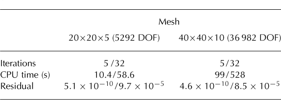
Table 3. Test C, L1 L2. Same quantities are reported as for Table 2

4.4. Test E: comparison of the FO and L1L2 models with the Stokes model
Test E is a 2-D problem in the x-z plane. The geometry is based on data from Haut Glacier d’Arolla, Switzerland; it has a horizontal extension of 5 km, shown in Figure 5. In order to reproduce a 2-D test with 3-D code, we take one layer of elements along the y direction and prescribe periodic boundary conditions on the artificial lateral surfaces. Two boundary conditions are considered. In the first case, no-slip boundary conditions are prescribed on the bedrock surface (Γ0 ≡ Γb). In the second case, we prescribe sliding boundary conditions, with β = 0 on the portion Γβ of the bedrock surface while on the remaining part (Γ0), no-slip conditions are prescribed; we set Γβ = {(x, z) ∊ Γb, 2.2 ≤ x ≤ 2.5 km}. As before, stress-free boundary conditions are prescribed on the top surface.
We first consider the FO model. The results shown are obtained with P2 elements on a 200 × 1 × 14 mesh. The horizontal velocity component, u, is reported in Figure 5. A one-dimensional plot of the surface velocity, u, as a function of x is shown in Figure 6 for the no-slip (left) and sliding (right) cases Both the FO solution (solid curve) and the Stokes solution (dashed curve) are reported. In this case, the bedrock has large slopes, hence the approximation hypotheses do not hold. However, we still have good agreement between the FO and Stokes solutions.

Fig. 5. Test E, FO model. The velocity component, u, on the x-z plane. The plot has been stretched by a factor 4 in the z direction for the sake of visualization. Left: no-slip. Right: partial sliding.

Fig. 6. Test E, FO model. The velocity component, u, on the surface as a function of x. (Dashed curve: reference Stokes solution. Solid curve: our FO solution.) Left: no-slip. Right: partial sliding.
Similar plots for the shear stress, τ xz , are shown in Figure 7. In the presence of sliding (right), the differences with the Stokes model are notable. However, it is worth mentioning that in the partial-sliding case, even the Stokes shear stress solutions included in the ISMIP-HOM benchmark were rather different from each other. This fact is clear from Figure 8, which shows the surface velocities (left) and basal shear stresses (right) computed by the Stokes models presented in the ISMIP-HOM benchmark. It can be seen that there is also a large variation in the velocity solutions. However, there are three FE models, namely ‘oga1’, ‘aas1’ and ‘mmr1’, which produce the same solution (up to a small tolerance). Moreover, the same Stokes velocity solution is reported in a recently submitted paper by Leng and others (personal communication from Lili Ju, 2011). Therefore, we believe that, even in the partial-sliding case, the surface velocity solution provided by the ‘oga’ group is reliable and it is reasonable to compare our model against it.

Fig. 7. Test E, FO model. The shear stress, τ xz , on the bed as a function of x. Left: no-slip. Right: partial sliding.

Fig. 8. Test E. Comparison between different Stokes solutions in the partial-sliding case. Left: the velocity component, u, on the surface. Right: the shear stress, τ xz , on the bed.
We next consider the L1L2 model approximation. The velocity component, u, at the surface and shear stress, τ xz , are reported in Figures 9 and 10, respectively. The reference Stokes solution is also reported. It is clear from these figures that the L1L2 model proposed is not adequate to solve test E. This could be partly expected since the problem features quite large aspect ratio and slope. We note that the shear stress, τ xz , at the bedrock has reasonable agreement with the Stokes solution, while the surface velocity is totally wrong. This could be due to the fact that in slow-sliding regimes, the L1L2 model cannot properly solve the boundary layer close to the free surface (see Reference Schoof and HindmarshSchoof and Hindmarsh, 2010). Moreover, in the partial- sliding case, the fast transition between slow- and fast-sliding regimes is difficult to account for by approximations of the Stokes model.

Fig. 9. Test E, L1L2 model. The velocity component, u, on the surface as a function of x. (Dash-dotted curve: L1L2 solution. Dashed curve: reference Stokes solution.) Left: no-slip. Right: partial sliding.

Fig. 10. Test E, L1L2 model. The shear stress, τxz, on the bed as a function of x. Left: no-slip. Right: partial sliding.
4.5. Test E: comparison between structured grids and a locally refined unstructured grid
Here we stress the fact that finite elements naturally handle nonuniform, unstructured grids. In order to show the potential of this feature, we compare the solutions computed with structured grids and an unstructured grid (Fig. 11, top left) which is refined in proximity to that part of the bedrock where free-slip boundary conditions are prescribed (partial- sliding case). The coarse-structure grid (Fig. 11, bottom left) has about the same number of nodes as the unstructured grid; precisely, the unstructured grid has 428 nodes while the structured grid has 394 nodes. However, the solution computed on the unstructured mesh is much more accurate than that computed with the coarse-structured mesh, and it is almost superimposed on the solution computed with the fine-structured grid (2978 nodes).
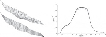
Fig. 11. Test E, partial-sliding case. Left: unstructured mesh (top) and coarse-structured mesh (bottom). Right: the velocity component, u, on the surface as a function of x, computed with FO model and P2 finite elements on different grids. (Dashed curve: unstructured mesh. Solid curve: fine-structured mesh (200 × 1 × 14). Curve with diamonds: medium-structured mesh (100 × 1 × 10). Curve with asterisks: coarse-structured mesh (50 × 1 × 7).)
4.6. Comparison between different first-order models
Here we compare our FO solutions with the solutions obtained using the FO approximation of the authors of the ISMIP-HOM paper (Reference PattynPattyn and others, 2008). Some of the ISMIP-HOM participants did not compute all the tests. Most of the FO models presented in the ISMIP- HOM were implemented using finite-difference methods, with the following exceptions: group ‘rhi’ uses spectral elements, while groups ‘cma’ and ‘bds’ use finite elements. We compare the models by looking at the usual plot of the velocity component, u, at the surface as a function of x for y = L/4 for test A (Fig. 12), test C (Fig. 13) and test E (Fig. 14). Unfortunately, the ‘rhi’ group did not perform test E.

Fig. 12. Test A. Comparison between our FO solution, the reference Stokes solution and the ISMIP-HOM FO models. The upper surface velocity component, u, is plotted as a function of x at y = L/4 for the two extremal lengths L = 5 km (left) and L = 160 km (right).

Fig. 13. Test C. Same quantities are plotted as for Figure 12.

Fig. 14. Test E. Comparison between our FO solution, the reference Stokes solution and those of the ISMIP-HOM FO models. The upper surface velocity component, u, is plotted as a function of x, at y = L/4 in the no-slip case (left) and in the partial-sliding case (right).
In the cases of tests A and C, we considered only the extremal lengths L = 5 and 1 60 km. On the 5 km geometry, test A (Fig. 12, left), no FO solution is close to the Stokes one. However, the ‘tpa1’ and ‘fpa1’ solutions are distinguished by being particularly far from it. The same phenomenon is present in test C (Fig. 13, left), where the ‘tpa1’ and ‘fpa1’ solutions are completely wrong, while the remaining models are quite close to the Stokes solution. For L = 160 km, test C (Fig. 13, right), we can see that most of the FO models are close to the Stokes solution with the exception of the ‘mtk1’, ‘cma2’ and ‘fsa1’ solutions. The ‘rhi2’ model and our model are the only ones that show good accuracy in both test A and test C on every length scale.
For test E (Fig. 14), most of the models give accurate solutions in the no-slip case. However, in the partial-sliding case a large variation in the solutions is registered. In this case, the only two FO solutions that are close to the Stokes solution are the ‘fpa1’ solution and our solution.
4.7. Comparison between different depth-integrated higher-order models
Here we compare the proposed L1L2 model with the depth- integrated higher-order models of the authors of the ISMIP- HOM paper (Reference PattynPattyn and others, 2008). Namely, we compare it with the L1 L1 and L1L2 models of group ‘rhi’ that are based on the work of Reference HindmarshHindmarsh (2004) and solved with spectral elements, the L1L2 model by group ‘dpo’ (Reference Pollard, DeConto, Hambrey, Christoffersen, Glasser and HubbardPollard and Deconto, 2007) solved with finite differences and the L1L1 model by group ‘lpe’ based on Reference MacAyealMacAyeal (1989) and Reference PattynPattyn (2003) and solved with finite differences. Because our L1 L2 method is devised for sliding boundary conditions, we only consider Test C. As before, we compare the models by plotting the velocity component, u, at the surface as a function of x for y = L/4. Figure 15 shows that our proposed L1L2 model performs well when compared with other higher-order models, for L ≤ 40. For L = 5, only the L1 L1 and L1 L2 models of group ‘rhi’ have good agreement with the reference solution, while our model presents a spurious bump in the solution.

Fig. 15. Test C. Comparison between our L1L2 solution (dash-dotted curve), the reference Stokes solution (dashed curve) and the L1L1, L1L2 models presented in the ISMIP-HOM benchmark. The upper surface velocity component, u, is plotted as a function of x at y = L/4 for different length scales. From left to right L = 5, 40 and 160 km.
4.8. Comparison between linear and quadratic approximations
Here we compare the FE solutions of the FO model obtained using different finite elements (P1 and P2) and different mesh sizes. We first consider test C (Fig. 16), for L = 5 km (left) and L = 160 km (right). The coarse mesh consists of 20 × 20 × 5 sub-cubes, for a total of 12 000 tetrahedra and 2624 vertices, whereas the fine mesh consists of 60 × 60 × 15 sub-cubes, for a total of 324 000 tetrahedra and 59 536 vertices. When using P1 elements, we have 5292 DOF for the coarse mesh and 119 072 DOF for the fine mesh. Using P2 elements, we have 36 982 DOF for the coarse mesh, and 907 742 DOF for the fine mesh.

Fig. 16. Test C. Comparison between solutions obtained using different finite elements (P1 and P2) and different meshes (40 × 40 ×10 and 60 ×60 × 15). Surface velocity component, u (top), and shear stress, txz , on the bed (bottom), as a function of x at y = L/4, for L = 5 km (left) and L = 160 km (right).
The upper surface velocity (Fig. 16, top) and shear stress, τ xz , on the bed (Fig. 16, bottom) are reported as a function of x at y = L/4. The velocity solutions are quite close to one another, even if the differences between the solutions are clear when the velocity scale is enlarged (Fig. 16, top left). Solutions on the coarse grid with P2 elements are comparable to those obtained with P1 elements on the fine mesh, but with one-third the number of DOF. Similar comparisons can be made for the shear stress. In the case L =160 km, the peak of the P2 shear stress on the coarse grid is lower than the correct one; however the overall P2 solution on the coarse grid is comparable with the P1 solution on the fine grid. We consider now test E (Fig. 17). We solve the problem on the coarse mesh, 50 × 1 × 7, and the fine mesh, 200 × 1 × 14. Remarkable differences between the solutions appear in the partial-sliding case (Fig. 17, right). Again, the solution computed with P2 elements on the coarse grid is comparable with the P1 solution on the fine grid.

Fig. 17. Test E. Comparison between solutions obtained using different finite elements (P1 and P2) and different meshes (50 × 1 × 7 or 200 × 1 × 14). Top: velocity component, u, on the surface. Bottom: shear stress, τxz . Left: no-slip. Right: partial-sliding.
5. Concluding Remarks
In this paper we have presented a parallel FE implementation of the fO model (Reference BlatterBlatter, 1995; Reference PattynPattyn, 2003; Reference Dukowicz, Price and LipscombDukowicz and others, 2010) and of the L1 L2 model (Reference HindmarshHindmarsh, 2004; Reference Schoof and HindmarshSchoof and Hindmarsh, 2010). We used three of the ISMIP- HOM tests to compare our results against a Stokes model. We showed that, in the case of the FO model, our solutions are very close to the Stokes solutions, except when the geometry featured large variations within a few kilometers (e.g. test A with L = 5, 10 km). Good agreement with the Stokes solution occurred also when performing the glacier test case, where the FO hypotheses (low aspect ratio, δ, and small slope) are only partially fulfilled. In the comparison with other FO models participating in ISMIP-HOM benchmarks, we find our FO model provides accurate results in the presence of sliding boundary conditions, whereas most of the others failed in at least one of tests C or E (section 4.6). The L1L2 model features good accuracy properties, again compared with other higher-order models, in the sliding case (test C) for L ≥ 40 km. However, the solutions can be very inaccurate for large aspect ratios and in the presence of no-slip boundary conditions (in this case the L1 L2 model reduces to the zeroth- order SIA model). Overall, the FO model showed itself to be more reliable than the L1 L2 model, while the latter has the obvious advantage of being computationally much cheaper.
Our model features both linear and quadratic finite elements. As expected, P2 elements produce more accurate solutions than P1 elements, in particular in the presence of large variations in the solution. This property can be exploited using coarser grids than those needed when using P1 elements. However, P1 elements feature fewer degrees of freedom, sparser matrices and do not need higher-order quadrature rules. Therefore, a comparison of the computational costs when using P1 and P2 elements is of paramount importance and will be addressed in a forthcoming paper.
Future work will consist of investigating the behavior of both our L1 L2 and FO higher-order models and the use of linear and quadratic finite elements on real geometries such as Greenland or Antarctica. The use of more realistic boundary conditions as well as a flow rate factor, A, dependent on the ice temperature will be considered. Although no substantial implementation-related difficulties are expected, a study of the possible effects on, for example, model stability and computational efficiency and accuracy, is called for. Future efforts will also be devoted to improving the efficiency and scalability of the solvers.
Acknowledgements
We thank Wei Leng for generating the meshes of Haut Glacier d’Arolla, A. Salinger for helping with NOX, and X. Asay-Davis, K. Evans, J. Nichols, W. Lipscomb and S. Price for fruitful discussions.
Appendix: Newton’S Method
The FO and L1 L2 models can be reduced to the solution of a nonlinear equation of the form F(u, v) = 0. In order to find the roots, (u, v), we use Newton’s method, which reads:
With ![]() Given an initial guess, (u
0, v
0), one solves Equation (A1) iteratively until ||F(uk
, vk
)||, in some norm, is less than a given tolerance (other stopping criteria are possible). The expression
Given an initial guess, (u
0, v
0), one solves Equation (A1) iteratively until ||F(uk
, vk
)||, in some norm, is less than a given tolerance (other stopping criteria are possible). The expression ![]() denotes the Gâteaux derivative of F in the direction
denotes the Gâteaux derivative of F in the direction ![]() evaluated at (u
k
, v
k
). The Gateaux derivative is a generalization of the concept of directional derivative. In particular if F were a vector function from ℝ2 to ℝ2, DF would be the Jacobian matrix in ℝ2x2 and the pairing (.,.) would represent the usual matrix vector product. We define the Gâteaux derivative as
evaluated at (u
k
, v
k
). The Gateaux derivative is a generalization of the concept of directional derivative. In particular if F were a vector function from ℝ2 to ℝ2, DF would be the Jacobian matrix in ℝ2x2 and the pairing (.,.) would represent the usual matrix vector product. We define the Gâteaux derivative as

In the following we derive the expression of the Gateaux derivative for the FO and L1 L2 models.
Gâteaux derivative for the FO model
Let F be defined as in Equation (16) (the dependence of F on (ϕ 1, ϕ 2) is understood). A direct computation of the limit in Equation (A2), gives

Where ![]() and
and

Gâteaux derivative for the L1L2 model
We consider the L1L2 model, with F defined as the left-hand side minus the right-hand side of the system of Equation (32), namely

A direct computation of the limit in Equation (A2) gives

where ![]() and
and

In the following we detail the calculation of (µ-1)
k
Differentiating both sides of ![]() with respect to
with respect to ![]()

and exploiting Equation (22) we have

In order to have an explicit expression for  we need to calculate
  To this aim we differentiate the squares of both sides of Equation (22) with respect to
 ![]()

Combining Equations (A9) and (A10) we get

The result, Equation (A7), follows straightforwardly since ![]() does not depend on z.
does not depend on z.


