


Introduction
During the last two decades there have been important advances in both the theory of glaciers (Reference Budd and RadokBudd and Radok, 1971; Reference LliboutryLliboutry, 1971 ) and the understanding of the characteristics and behaviour of polar glaciers and ice sheets (Reference Sugden and JohnSugden and John, 1976). However, with some notable exceptions (for instance Reference BoultonBoulton, 1972[a]; Reference HughesHughes, 1973; Reference Boulton, Boulton, Jones, Clayton, Kenning and ShottonBoulton and others, 1977; Reference SugdenSugden, 1977), there have been few attempts to apply this knowledge to explaining form–process relationships in areas of mid-latitude Pleistocene glaciation, despite the fact that glacier conditions will tend to be a crucial set of variables. In the context of glacial erosion, variables which have been emphasized in the past have included bedrock structure (Reference LjungnerLjungner, 1930; Reference LarssonLarsson, 1954; Reference LewisLewis, 1954; Reference ZumbergeZumberge, 1955), pre-glacial relief (Reference KlimaszewskiKlimaszewski, 1964), time and landform evolution (Reference DavisDavis, 1900; Reference Linton, Priestley, Priestley, Adie and RobinLinton, 1964, Reference Linton, Wright and Osburn1968), ice-flow patterns (Reference McCall and LewisMcCall, 1960; Reference Nye and MartinNye and Martin, 1968), ice discharge (Reference PenckPenck, 1905; Reference BlacheBlache, 1952), pre-glacial weathering (Reference BakkerBakker, 1965; Reference FeiningerFeininger, 1971), and periglacial weathering (Reference BoyéBoyé, 1968). While such factors are undoubtedly important at a local scale, one of the fundamental constraints on effective glacial erosion appears to be glacier thermal regime and the requirement for basal ice to be at the pressure-melting point, so that basal slip occurs (Reference BoultonBoulton, 1972[b]). Reference AndrewsAndrews (1972), for example, has suggested that rates of erosion might differ by an order of magnitude between cold-based high-Arctic glaciers and warm-based temperate glaciers. In Greenland, Reference SugdenSugden (1974) demonstrated a general relationship between zones of glacial erosion and basal ice conditions. Areal scouring occurred mainly in the south-west and was thought to reflect the former presence of basal ice at the pressure-melting point; landscapes with no signs of glacial erosion related to areas where the basal ice was below the pressure-melting point.
Areal scouring, or “knock-and-lochan” topography (Reference LintonLinton, 1963), is one of the classic forms of glacial erosion, comprising ice-scoured and quarried rock bosses and closed basins often showing a close relationship to bedrock structure. If effective glacial erosion is related to basal ice at the pressure-melting point, then areal scouring may be expected to correlate with the latter. It is the aim of this paper to test the hypothesis that there is a spatial correlation in an area of Pleistocene glaciation between zones of reconstructed basal-ice melting and landscapes of areal scouring. Basal-ice temperatures are predicted from glacier theory for a west to east transect across a northern dome of an equilibrium Scottish ice sheet at its maximum extent (Fig. 1) and compared with the distribution of areal scouring. It should be noted that this is only one of many possible transects across a former Scottish ice sheet, and the results are not necessarily applicable elsewhere particularly since the Scottish ice sheet was not a simple feature but probably consisted of several coalescent units or domes.

Fig. 1. Ice flow-line model and limits for the ice maximum (based on Reference FlintFlint ([c1971]), Reference HoppeHoppe (1974), Reference Clapperton, Sugden and GemmellClapperton and Sugden (1975), and Reference SissonsSissons ([c1967], [c Reference Sissons1976])). The cross-profile in Figure 2 is denoted by the line ab.
Glacier Temperature-Profile Models
Glacier temperatures are related to heat from four sources: the geothermal flux, internal deformation, basal sliding, and surface warming (Reference PatersonPaterson, 1969). Temperature distribution in a vertical dimension in an ice sheet was considered by Reference RobinRobin (1955) and he derived a solution for the heat-transfer and temperature-profile equation. This solution is for a steady-state, cold-based ice sheet. As it does not include the effects of warming due to frictional heating, it is only applicable to the central area of an ice sheet where velocities tend to be low. Incorporating frictional heating, Reference Jenssen and RadokJenssen and Radok (1963) obtained numerical solutions for particular profiles, while Reference WeertmanWeertman (1961) and Reference ZotikovZotikov (1963) discussed solutions for basal ice at the pressure-melting point and the threshold ice thickness at which basal melting occurred. More recently, from a review and analysis of heat-transfer theory, Reference BuddBudd (1969) derived a general solution for the temperature profile of a steady-state ice cap including the effects of horizontal and vertical motion, conduction, and accumulation. Subsequent work by Reference Budd, Budd, Jenssen and RadokBudd and others (1971[a]) saw the development of more sophisticated models for ice-sheet temperature distribution. In their fixed-column model, the heat-conduction equation is solved for a vertical column of ice. When applied to known temperature profiles from the Greenland and Antarctic ice sheets, it gave satisfactory results (Reference Budd, Budd, Jenssen and RadokBudd and others, 1971 [b]) and it is used in the present study. The basal temperature θ b is given by

in which θ s is the mean ice-surface temperature, Z is the ice thickness, γ b is the basal temperature gradient, γ s is the ice-surface temperature gradient and y is a dimensionless thermal parameter. The assumptions of the model are as follows:
-
(a) Conduction occurs in a vertical sense only.
-
(b) The advection rate throughout the column is constant and equal to the surface warming rate.
-
(c) All the frictional heat is applied at the base of the glacier and is not distributed throughout the ice. Reference BuddBudd (1969) considered this to be a reasonable approximation, and his calculations for a power flow law of ice demonstrated a concentration near the base of heat production due to friction.
-
(d) The ice sheet is in a steady-state.
-
(c) The strain-rate is constant.
-
(f) The thermal diffusity of the ice is constant.
-
(g) Temperatures are steady-state.
-
(h) Basal melting does not occur.
Reference Radok, Radok, Jenssen and BuddRadok and others (1970) discussed the effects of variations in the input parameters on the temperature profile. As temperature in a cold ice sheet generally increases with depth due to geothermal heating at the base, high values of ice thickness will tend to give large differences between surface and basal temperatures. Therefore, basal melting is more likely to occur under thick than thin ice, particularly if the surface warming-rate is high. A high basal temperature gradient has the effect of increasing the basal temperature in a positive direction relative to the surface temperature, while a high accumulation rate will lower the temperature difference between surface and base. In addition, if y is high in value, either through high values of accumulation rate or ice thickness of which it is a function, then y −1 erf y is relatively small, and E(y) is relatively high. In such a case, the product of the latter, and the negative surface gradient will be relatively high in comparison with the product of the former and the positive basal gradient, and basal temperature will be relatively colder than surface temperature.
Derivation of Temperature Model Inputs for a Former Scottish Ice Sheet
Ice thickness
To estimate ice thickness, the former ice-surface profile was reconstructed from the parabolic solution of Reference NyeNye (1952). The height h of a point on the ice-sheet surface is given by
in which s is the horizontal distance from the ice-sheet edge to the point of measurement of h. The term h 0 is given by′

in which τ is the basal shear stress, ρ is the density of ice and g is gravitational acceleration. A constant shear stress of 1 bar was assumed, and in this case h 0 is equal to 11 m.
To derive the parameter s, it is necessary to know the limits of the Scottish ice sheet. At its maximum extent, the western edge of the ice probably lay between the Flannan Isles and St. Kilda (Reference SissonsSissons, [c1967]). The exact limit was assumed to coincide with the 50 fathom (91 m) bathymetric contour west of South Uist. This corresponds to the estimated maximum sea-level lowering of 90 m during the Pleistocene (Reference FlintFlint, [c1971]). From evidence of glacial breaching and distribution of erratics, the central axis of the ice sheet in north-west Scotland is thought to have been located to the east of the present watershed (Reference DuryDury, 1953; Reference SissonsSissons, [c1967]). However, it probably occurred not too far to the east since there is evidence of eastward movement of ice in northern Scotland (Reference SissonsSissons, [c1967]). In the model, the iceshed was located 12.5 km cast of the highest mountains in the transect and approximately 20 km east of the present watersheds in Glen Affric and Glen Shiel (Fig. 4). As the eastern limits of the Scottish ice in the North Sea remain conjectural, that part of the eastern profile relevant to the area studied was obtained by symmetrical extrapolation of the western one.
In estimating ice thickness, isostatic depression of the land surface was assumed. Since basal temperatures were to be calculated for a relatively central area in terms of the whole ice sheet, and since isostatic adjustment does not reflect local topographic effects on loading (Reference FlintFlint, [c1971]), an average value was estimated for isostatic depression. The difference between the ice-surface and present ground-surface altitude was averaged for 41 points over a distance of 50 km on each side of the ice centre along the line of profile. The figure obtained is equivalent to 0.733 times the average ice thickness assuming isostatic depression of 0.267 times the ice load (Reference Brotchie and SilvesterBrotchie and Silvester, 1969). This gave a value of 1276 m for the average ice thickness and 465 m for the average isostatic depression under the central area of the ice sheet.
Ice-Surface Temperature
An estimate of −2°C was made for the mean annual sea-level temperature at the western margin of the ice sheet. This represents a lowering of 10.5 deg below the mean annual temperature for Stornoway in the Outer Hebrides during the period 1931–51 (Great Britain. Meteorological Office, 1963) and is of the magnitude suggested by Reference FlintFlint ([c1971]) for the ice maximum in Britain. More extreme conditions have been suggested by Reference Coope, Coope, Morgan and OsborneCoope and others (1971) and Reference Williams, Wright and MoseleyWilliams (1975) for the English Midlands at the ice maximum, and during the late-glacial Loch Lomond stadial, the presence of permafrost features in Mull suggests a mean annual temperature for western Scotland of no higher than −1°C and probably lower (Reference SissonsSissons, [c1976]). Therefore, the above estimate is probably a conservative one. Surface temperatures across the ice sheet were estimated using a lapse-rate of 7 × 10⁻³ deg m−1. This is the mean value used by Reference DiamondDiamond (1960) to compute mean annual air temperatures for areas of the Greenland ice sheet where air and ice temperatures were not available.
Basal Temperature Gradient
The basal temperature gradient γ b is given by the sum of the geothermal heat gradient and the internal frictional heat gradient produced by glacier movement:

in which γ G is the geothermal heat gradient, V is the ice velocity, J is the mechanical equivalent of heat, and K is the thermal conductivity of the ice. A minimum value of 1.4 μcal cm−2 s−1 (5.9 μJ cm−2 s−1) was estimated for the geothermal heat flux for northern Scotland from Lee and Uyeda (1965, fig. 44). The thermal conductivity of the ice is temperature-dependent, and a value of 5.4×10⁻³ cal cm−1 s−1 deg−1 (22.6×10⁻³ J cm−1 s−1 deg−1) was selected as an average for temperatures in the range 0° to −10°C. The mean velocity V of the ice column was estimated as that required to maintain the ice sheet in a balanced state:

in which x is the distance from the ice-sheet centre, Āx is the mean accumulation over this distance and Z is the ice thickness.
Surface Warming Rate
Because of the decrease in ice-surface temperature with increasing altitude, there is a corresponding variation in the temperature of the accumulating firn. Due to the movement of ice both downwards and outwards from the ice-sheet centre, each annual layer of firn accumulates at a slightly warmer temperature than the previous one. This surface warming rate is expressed as Vαλ, and the negative surface-temperature gradient γ s, by the formula of Reference RobinRobin (1955), as

in which α is the ice-surface gradient, λ is the lapse-rate, and A is the accumulation rate.
Accumulation Rate
Mean annual precipitation for the central area of the ice sheet at the ice maximum was estimated at 100 cm from the maps of values predicted by Williams and Barry (1974) from their simulation of Ice Age climate using the NCAR global circulation model. This value was also assumed to be the mean annual accumulation.
Additional Parameters
The dimensionless thermal parameter y is given by
in which κ is the thermal diffusivity of the ice. κ is temperature-dependent, and a value of 1.2 × 10⁻² cm2 s−1 was selected for temperatures in the range 0° to −10°C.
The function erf y is defined as

The function E(y) is the integral

in which F(x) is the Dawson Integral

Values of these functions have been tabulated by Reference Abramowitz and StegunAbramowitz and Stegun ([1965]) and graphed by Reference BuddBudd (1969).
Derived Basal Temperature Conditions
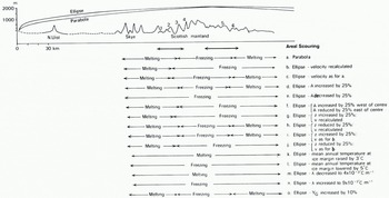
Derived basal temperature conditions are shown in Figure 2a, and input values for a selection of points in Table I. The pattern of basal thermal regime is that of a cold-based central area approximately 55 km in width succeeded by zones of basal melting towards both the east and west. This reflects an increase in ice thickness as the underlying relief decreases towards the present coast and also an increase in basal temperature gradient as velocity increases away from the centre. The negative surface-temperature gradient also increases away from the centre but at a slower rate than the basal one.
Table I. Temperature-Model Input Values for Selected Sites at the Ice Maximum (Parabolic Ice-Surface Profile)

Effects of Varying the Model Inputs
In view of the assumptions involved in estimating the input parameters, it is instructive to consider the effects of varying the latter.
Form of the Ice-Surface Profile
The parabolic profile used tends to be steeper than ice-sheet profiles observed in reality. Basal temperatures were therefore calculated for a flatter elliptical profile of the form

in which h is the ice thickness at a distance x from the ice centre, L is the half-width of the ice sheet, and Z is the ice thickness at the ice-sheet centre. Average isostatic depression was estimated in this case to be 496 m for the central area. One effect of this model is progressively to increase the ice thickness away from the centre which reduces the ice velocity and therefore also the basal-temperature gradient. The surface-temperature gradient is also reduced but to a lesser extent. A further effect is to lower the ice-surface temperature away from the centre, since the surface profile is at a relatively higher altitude. The combined effects of these changes on basal temperatures are small and of the order of −1 deg which extends slightly the central area of basal freezing particularly in the east (Fig. 2b). If the ice velocity is held constant, there is a slight increase in the extent of basal melting (Fig. 2c).
Annual accumulation rate
An increase of 25% in the annual accumulation rate increases the ice velocity and hence the basal temperature gradient. This in turn decreases the extent of the central freezing zone (Fig. 2d). A decrease of 25% in the annual accumulation rate produces the opposite effect (Fig. 2e). Initially, accumulation was assumed constant across the central area of the ice sheet. A more realistic pattern may be one of precipitation decreasing both with altitude in towards the ice centre and with increasing distance from maritime sources in the west. This reduces the extent of the central zone of basal freezing west of the ice centre and increases it to the east (Fig. 2f).
Ice thickness
An increase of 25% in ice thickness reduces the ice velocity and therefore the basal temperature gradient. The result is to reduce slightly the basal temperatures and increase the extent of the central area of basal freezing (Fig. 2g). Decreasing the ice thickness by 25% produces the opposite effect (Fig. 2h). If the ice velocity is held constant, an increase in ice thickness reduces the extent of the basal freezing and vice versa (Fig. 2i and j).
Surface temperature
An increase of 3 deg in the mean annual temperature at the western edge of the ice sheet is sufficient to raise the whole of the central area of the ice sheet to the pressure-melting point at its base (Fig. 2k); a decrease of 5 deg is sufficient to extend the central zone of basal freezing beyond the area considered (Fig. 2l). Decreasing the ice-surface temperature lapse-rate from 7 × 10⁻³ deg m−1 to 4 × 10⁻³ deg m−1 would raise the whole of the central area to the pressure melting point (Fig. 2m); increasing it to 9 × 10⁻³ deg m−1 would produce basal freezing over the whole of the area considered (Fig. 2n).
Geothermal heat flux
The value of the geothermal heat flux used in the model is a minimum value for northern Scotland (from Reference Lee, Uyeda and LeeLee and Uyeda, 1965). Increasing it by 10% reduces the extent of the central zone of basal freezing (Fig. 20).
Summary
These additional calculations suggest that errors in estimating ice thickness, accumulation rate, and the geothermal heat flux do not affect greatly the predicted pattern of ice-sheet thermal regime of a central area of basal freezing succeeded by zones of basal melting to the west and east. Only small changes occur in the positions of the zone boundaries. However, errors in the estimates of mean annual temperature at the ice margin and ice-surface temperature lapse-rate will have much more significant effects and, depending on their magnitude and direction, basal thermal conditions might range from completely freezing to completely melting over the area considered.
The Distribution of Areal Scouring
The distribution of areal scouring was mapped from air photographs and field work. A typical ice-scoured landscape is shown in Figure 3. Areal scouring occurs in two broad zones, one to the west and one to the east of the central mountain belt (Fig. 4). In the west, typical ice-scoured topography extends from sea-level at the western limits of the Kyle of Lochalsh and Glenelg peninsulas eastward to about 900 m o.d. on The Saddle and A’ Ghlas-beinn. The summit of the latter (916 m. o.d) is scoured and ice-roughened, but the adjacent plateau of Beinn Fhada rising to 1032 m o.d. is comparatively smooth in outline. Farther east, the high ridges flanking Glen Shiel, Glen Affric, and Glen Cannich are rocky and frost-riven in places but they do not display the typical scoured forms of the west. Locally, however, scouring is present on cols (for example just to the east of The Saddle), in areas of convergent ice streams (for example to the south-west of upper Glen Elchaig) and along the flanks of the glens which acted as major ice-discharge routes.

Fig. 3. Landscape of areal scouring near Glenelg. (Crown copyright reserved.)

Fig. 4. Distribution of areal scouring in a transect across northern Scotland.
To the east of the mountains, on the plateau north of Glen Cannich, the summits of Càrn nan Gobhar (991 m) and Creag Dhubh (946 m) are unscoured although their lower spurs display the typical forms. It is only farther east at An Soutar (676 m) that the plateau itself becomes extensively scoured. South of Glen Cannich, the summit of Toll Creagach (1052 m) is smooth and regular in outline. However, immediately to the east the plateau is scoured from Doire Tana (892 m) eastward. South of Glen Affric, scoured forms are present on the summit of Càrn Glas Lochdarach (771 m) but absent from the slightly higher Aonach Shasuinn (884 m). To the north-east, the trough form of Glen Afiric opens out along its south side as a relatively low, linear depression over which scouring extends from Loch Beinn a’ Mheadhoin to the interfluve at around 450 m. On the extensive plateau surfaces of Guisachan, Balmacaan and Dundreggan Forests to the east of Glen Affric, areal scouring is again the predominant landscape form. Between Glen Affric and the River Enrick, relief amplitude is low and peat moors blanket much of the bedrock. East of the river, however, a relatively higher scoured surface occurs with rocky hills up to 150 m in amplitude in the case of Meall a’ Chràthaich (678 m o.d.). Prominent lineations in this area reflect underlying bedrock structures.
The distribution of areal scouring thus tends to be associated with topographic surfaces below about 900 m in altitude. Distance from the main mountain mass may also be a related factor but it is itself correlated with topographic altitude.
Relationships of Areal Scouring to Reconstructed Ice-Sheet Basal Temperatures
Areal scouring to the west of the mountains spatially coincides in part with predicted areas of basal melting for the parabolic and elliptical ice-surface profile models and also under conditions of increased accumulation rate, geothermal heat gradient, and ice thickness (velocity held constant) (Fig. 2). If the ice were thinner, accumulation rate lower, lapse-rate higher, or mean annual temperature at the ice margin lower, then no correlation would exist. To the east of the mountains there is little spatial correlation between zones of basal melting and areal scouring (Fig. 2). It is only under conditions of increased ice thickness and accumulation rate that the eastern part of the scouring becomes associated with basal melting. The greater part of the scouring here does not correspond with the basal melting under any of the conditions modelled. This relates to the location of the eastern scoured zone close to the centre of the ice sheet where predicted ice velocities, surface temperatures, and ice thicknesses are relatively low.
It may be that the most effective conditions for glacial erosion were not associated with the ice maximum but with intermediate stages in the growth or decay of the ice sheet. To investigate this possibility, basal temperatures were calculated for an ice sheet of half the original width and with the same temperature and accumulation rate inputs as for the original calculation (Fig. 5; Table II). The resulting pattern of basal thermal regime is broadly similar to that of the ice maximum; a central zone of basal freezing and outer zones of basal melting both to the east and west. The central freezing zone is less extensive than before but still extends across the eastern area of areal scouring. However, if the iceshed is assumed to be located over the mountains rather than to the east of them, which might tend to be the situation during the early build-up of the ice sheet, then basal melting is predicted to coincide with the eastern scoured zone as well as with the western one.

Fig. 5. Reconstructed thermal conditions for an ice sheet of half the estimated ice-maximum width.
Table II. Temperature-Model, Input Values for Selected Sites (Ice Sheet Half Estimated Maximum Size)

Conclusion
1. Reconstructed ice-sheet temperatures for a transect across northern Scotland suggest the former presence of a central area of basal freezing reflecting low values there of ice velocity, surface temperature, and ice thickness. As predicted values of these variables increase in magnitude away from the centre both to the west and east, basal temperatures tend to rise. Whether or not the pressure-melting point was reached appears to depend critically on the input values of mean annual temperature at the ice margin and ice-surface temperature lapserate. No local data are available for either at the ice maximum. When compared with data from the English Midlands for the same period (Reference Coope, Coope, Morgan and OsborneCoope and others, 1971; Reference Williams, Wright and MoseleyWilliams, 1975), the estimate of mean annual temperature is seen to be relatively high, even allowing for some possible ameliorating maritime influence. (Reference Williams, Barry, Weller and BowlingWilliams and Barry (1974) suggested that the latter may have been greatly reduced at the ice maximum.) The most probable temperature reconstruction for the ice maximum in the light of present knowledge is therefore basal freezing over the entire area of the mainland considered. This is also the pattern predicted by Reference Boulton, Boulton, Jones, Clayton, Kenning and ShottonBoulton and others (1977). Basal melting seems most likely to have developed, if at all, either during ameliorating climatic conditions following the ice maximum or during periods of less extensive ice advance associated with climatic conditions less severe than those predicted for the ice maximum.
2. Even under the most favourable conditions for basal melting modelled, there is only a partial spatial correlation between areal scouring and warm-based ice in the west and little or none in the east for the ice maximum. This may be explained in several ways:
-
(a) The temperature-profile model is wrong or incomplete (see Reference HookeHooke, 1977).
-
(b) The model inputs are wrong.
-
(c) Areal scouring in northern Scotland is not related to the former presence of warm-based ice.
-
(d) The formation of areal scouring in northern Scotland is not related to predicted glaciological conditions at the ice maximum.
-
(e) The formation of areal scouring is spatially and temporally transgressive during the build-up and decay of ice sheets in northern Scotland.
Of these, the fourth and fifth seem to be the strongest possibilities. As the ice built up and decayed through time, zones of different basal temperature conditions are likely to have been spatially transgressive. Also during ice build-up and following the ice maximum, surface temperatures are likely to have been higher, tending to favour basal melting.
3. The focus in the present study on trying to link glacier theory and geomorphology has raised new questions and problems, and may offer a productive line of approach to understanding the complex form–process relationships in formerly glaciated areas. Computer simulation of the continuous build-up and decay of former ice sheets offers exciting possibilities and may overcome the problems of attempting to correlate “static” landform patterns in the present landscape with dynamic glaciological conditions and processes.
Acknowledgements
The work reported in this paper was carried out in the Department of Geography, University of Aberdeen, during the tenure of a Natural Environment Research Council Studentship which the author gratefully acknowledges. It is also a pleasure to thank Dr D. E. Sugden for many stimulating discussions and for commenting on a draft of the manuscript.


