


1. Introduction
Some glaciers are known to surge periodically, a phenomenon that has long intrigued glaciologists and is the subject of extensive studies and reviews (Meier and Post, Reference Meier and Post1969; Clarke, Reference Clarke1987; Raymond, Reference Raymond1987; Harrison and Post, Reference Harrison and Post2003). Although many mechanisms may contribute to the initiation and termination of the surge, such as the drainage switch (Kamb and others, Reference Kamb1985; Murray and others, Reference Murray, Strozzi, Luckman, Jiskoot and Christakos2003; Benn and others, Reference Benn, Fowler, Hewitt and Sevestre2019), the till instability (Kamb, Reference Kamb1991; Boulton and others, Reference Boulton1996; Nolan, Reference Nolan2003; Minchew and Meyer, Reference Minchew and Meyer2020) or the pulsed englacial water storage (Lingle and Fatland, Reference Lingle and Fatland2003), the thermal switch (Clarke, Reference Clarke1976; Fowler and others, Reference Fowler, Murray and Ng2001) remains one of the most viable in producing the self-oscillation.
At its most basic, the thermal switch operates as follows (MacAyeal, Reference MacAyeal1993): when a glacier thickens by accumulation, the increasing sequestration of the geothermal heat would warm its bed to the pressure-melting point and the ensuing production of meltwater would weaken the bed to trigger a sliding motion. This fast flow would thin the glacier and augment the conductive cooling of the bed, leading to its freezing that terminates the surge. Our aim is to consider a minimal yet physically closed thermal switch to see if it can explain the behavior of diverse glaciers.
Given its robustness, any model that entails the basic thermal switch would produce a surge cycle, as amply demonstrated in numerical studies. For a quantitative simulation however, the critical element is the sliding velocity where primary uncertainty arises. In some models, this sliding velocity is simply imposed as a jump or triple-valued function of the basal stress (Payne, Reference Payne1995; Calov and others, Reference Calov, Ganopolski, Petoukhov, Claussen and Greve2002; Sayag and Tziperman, Reference Sayag and Tziperman2009; Kyrke-Smith and others, Reference Kyrke-Smith, Katz and Fowler2013), and in others, it has evolved into a sliding flow law (Budd and others, Reference Budd, Jenssen and Smith1984; Bentley, Reference Bentley1987) that remains in wide use to this date (Dunse and others, Reference Dunse, Greve, Schuler and Hagen2011; Feldmann and Levermann, Reference Feldmann and Levermann2017; Smith-Johnsen and others, Reference Smith-Johnsen, Schlegel, de Fleurian and Nisancioglu2020). This sliding flow law links the sliding velocity to the effective pressure, which rightfully underscores the importance of the subglacial hydrology, but it contains a sliding parameter that can be arbitrarily set to produce the desired sliding velocity. As the latter directly impacts the amplitude and period of the surge cycles, it renders such models practically unfalsifiable by observations.
The presence of such a free parameter is clearly indicative of missing physics, which can be bridged by two recent advances. First, laboratory experiments show that subglacial till responds to a shearing stress plastically with a yield strength that is a function only of the effective pressure (Iverson and others, Reference Iverson, Hooyer and Baker1998; Tulaczyk and others, Reference Tulaczyk, Kamb and Engelhardt2000a), and once the driving stress exceeds the yield strength, the ice begins to slide and its motion becomes decoupled from the basal stress. This laboratory finding is also supported by field observations (Iverson and others, Reference Iverson, Hanson, Hooke and Jansson1995; Whillans and van der Veen, Reference Whillans and van der Veen1997; Bennett, Reference Bennett2003), which plainly invalidates the local sliding flow law. The second advance concerns the excess driving stress, which is seen from the field data to be taken up by the side drag, and the accompanying lateral strain may account for the observed sliding velocity (Echelmeyer and others, Reference Echelmeyer, Harrison, Larsen and Mitchell1994; Whillans and van der Veen, Reference Whillans and van der Veen1997; Joughin and others, Reference Joughin, Tulaczyk, Bindschadler and Price2002). The empirical sliding flow law thus can be replaced by the global momentum balance and the nominal viscous flow law, which contain no free parameter except for the introduction of the glacial width that is set by the bed trough.
With the above, we see that a prognostic model of the surge cycles must include the global momentum balance and the subglacial hydrology, and a closed set of equations has been assembled by Tulaczyk and others (Reference Tulaczyk, Kamb and Engelhardt2000b), a formalism known as the ‘undrained plastic bed’ (UPB). We shall employ this formalism in this paper for which the ‘undrained’ assumption can be justified by the curbing of the lateral meltwater dispersal by the topographic trough. Such lateral drainage however plays a key role in Part 2 (a future paper) in constraining the ice stream width.
Employing the UPB, numerical calculations have produced realistic surge cycles, whose dependence on the external condition, however, is not addressed by Bougamont and others (Reference Bougamont, Price, Christoffersen and Payne2011) and only in a limited fashion by Robel and others (Reference Robel, DeGiuli, Schoof and Tziperman2013). The latter have singled out ice surface temperature and geothermal heat flux in assessing the boundary separating the cyclic-surge and steady-sliding regimes; and since their formulation is predicated on a sliding glacier, it cannot address the long-standing question of what distinguishes the surge-type from normal glaciers. This question is brought to the forefront by recent censuses of glaciers (Sevestre and Benn, Reference Sevestre and Benn2015), which discerned markedly the external control by the regional climate and glacier geometry. A quantitative comparison with this observation should provide a potent test of our model.
In view of the foregoing shortfalls and promises, we seek to reformulate Robel and others (Reference Robel, DeGiuli, Schoof and Tziperman2013) to incorporate the steady-creep regime and broaden the external dependence of the glacial behavior to both the regional climate and the glacier size. A tangible outcome of the study is the construction of a 2-D regime diagram that allows a ready prognosis of the glacial properties over the full range of the external conditions – both climate- and size-related. As a significant extension, this regime diagram will be applied to observed glaciers of diverse behaviors, possibly unifying their dynamics.
The UPB of fixed glacier width obviously does not apply to flat-bed ice streams of unknown width, such as Ross ice streams. This is the subject of Part 2 wherein we posit that the ice discharge would self-organize into alternating streams, with their width constrained by the hydraulic conductivity. The integration of the surge cycles and self-organization into the same theoretical framework would further sharpen our understanding of the glacial dynamics.
For the organization of this Part 1, we introduce the model in Section 2 and formulate it in Section 3 via the consideration of a prototypical surge cycle. We then construct a regime diagram in Section 4 to assess the glacier properties and their external dependence. In Section 5, we apply the regime diagram to representative glaciers for quantitative comparisons. We provide further discussion in Section 6 and summarize the main findings in Section 7.
2. Model
As sketched in Figure 1, we consider a glacier or ice stream confined in an idealized topographic trough of constant depth (dashed). The greater glacial depth hence driving stress propels a faster flow, which is bounded on the side by a stagnant ice sheet. Since the driving stress is broadly peaked between the reservoir and receiving zones where the surge is likely triggered (Bindschadler and others, Reference Bindschadler, Bamber, Anandakrishnan, Alley and Bindschadler2001), the model variables pertain to this middle section (shaded) where the thermal switch is the most active to endow the primary glacial behavior. As such, we are not addressing the longitudinal variation associated with advection or the kinematic wave (Nye, Reference Nye1960; Clarke and others, Reference Clarke, Collins and Thompson1984), and the longitudinal dimension enters only through the glacier half-length l (all symbols are listed in the Appendix), which we take to be the proper scale for the catchment distance and in defining the surface slope. The catchment contribution from tributaries or the inward entrainment can be absorbed into this scale. This is the spatial-lumped model commonly used in assessing the surging behavior.

Fig. 1. Model glacier confined in a topographic trough (dashed) bounded on the side by the stagnant ice sheet. The model variables pertain to the middle section (shaded) between the ice divide and the terminus, with h, w and u being the thickness, the half-width and the velocity of the glacier, respectively, and the half-length l defines both the catchment distance and the longitudinal scale.
To consolidate the external dependence, the state variables will be non-dimensionalized; but given the widely varying glacier sizes even in the same climate zone, we shall define the scales by the climate condition and derive the solution as a function of the scaled glacier dimensions. This non-dimensionalization scheme is seen later to facilitate the construction of a 2-D regime diagram, which allows an easy prognosis of the glacier behavior over the full range of the external conditions – both climate- and size-related. In the following, the scales are indicated by brackets and the non-dimensionalized variables by primes.
3. Surge cycle
The model is formulated through the consideration of a prototypical surge cycle, as shown in Figure 2 in the phase space of scaled glacier thickness (h′) and ice flux (q′). The figure is based on the solution of an actual glacier in Svalbard (Section 5). It consists of slow-creep and fast-sliding phases and instantaneous onset and termination of the sliding, with the transition stages numbered for reference.

Fig. 2. Surge cycle on a phase space of non-dimensionalized ice flux (q′) and glacier thickness (h′). It consists of slow-creep, fast-sliding and instantaneous onset and termination of the sliding, separated by the numbered stages. If the catchment flux (vertical dashed line) intersects the creep or sliding phase, it would yield a steady state. The figure is based on the model solution of a Svalbard glacier.
Following the start of the creep (stage 1), the glacier thickens by accumulation, accompanied by increasing driving stress hence ice flux. The geothermal heating, increasingly sequestered by the thickening ice, would warm the bed to the pressure-melting point when the sliding is initiated (stage 2). The enhanced frictional heating and meltwater production would weaken the bed, and the excess driving- over basal-stress would accelerate the sliding motion until it is curbed by the side drag (stage 3). During the sliding phase, the fast flow would lower the glacier surface accompanied by decreasing driving stress and ice flux. When the thinning-enhanced conductive cooling exceeds the basal heating, the bed would freeze to terminate the sliding (stage 4). The glacier then reenters the creep phase (stage 1), thus completing the cycle.
The surge cycle obviously would not materialize if the ice flux during creep or sliding phases is arrested by the catchment flux indicated by the vertical dashed line, in which case a steady state would ensue. These additional regimes of steady-creep and steady-sliding will be discussed in the next section, but for now we assume the catchment flux to lie between ice fluxes of the two phases so as not to affect the surge cycle and proceed to derive the state variables through the cycle.
3.1 Creep phase
To seek a thickness scale that depends only on the climate condition, we take it to be the glacier thickness at stage 2 when the bed first becomes temperate. Since the glacial surface is rising prior to stage 2 with minimal downward cold advection, we assume the englacial temperature to be in conductive equilibrium with the geothermal flux, as shown by the thick solid line marked ‘2’ in Figure 3. It is at the pressure-melting point (T m) at the bed and has a constant slope given by the ‘geothermal’ lapse rate $\gamma _{\rm g} = \dot{g}( {\rho_{\rm i}c_{p, {\rm i}}K} ) ^{{-}1}$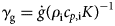 with $\dot{g}$
 being the geothermal flux, ρ i and c p,i, the density and specific heat of ice, and K, the thermal diffusivity, respectively. Drawn in the thin line is the temperature when the snow is deposited, which thus assumes the winter air temperature with its sea-level value T a (Only the air temperature above the surface at stage 1, same as stage 4, is of relevance and we have assumed a glacier bed at the sea level for simplicity; the latter can be adjusted for individual applications) and a constant atmospheric lapse rate γ a.
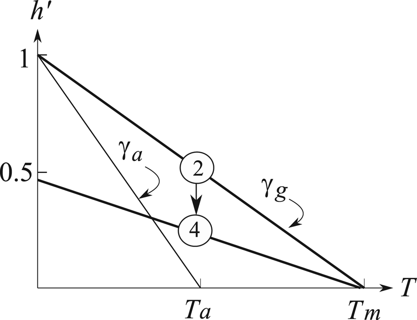
Fig. 3. Pre-sliding (stage 2) and post-sliding (stage 4) temperature profiles in thick lines. The former is characterized by the geothermal lapse rate γ g and a bed temperature at the pressure-melting point T m. This profile is steepened by the sliding-induced thinning (the arrow) to that of stage 4 when the sliding terminates. The thin line is the winter air temperature when the snow is deposited, which has a sea-level temperature T a and a constant atmospheric lapse rate γ a.
Since the geothermal lapse rate is steeper than the atmospheric lapse rate, the bed warms during the surface growth and attains the pressure-melting point when the thickness reaches:

Other than the geothermal flux fixed by the geomorphology, this thickness depends only on the climate condition, it thus meets our scaling criteria to be set as the thickness scale (hence bracketed). Expectedly, a warmer climate or greater geothermal flux would yield a thinner glacier when its bed becomes temperate.
We now seek a distance scale [l] that also depends only on the climate condition. One natural choice is the catchment distance that would be in mass balance with the thickness scale. But to apply the mass balance, which involves the ice flux, we need to first define some interim scales, as seen next. Since the driving stress is of the form

where g is the gravitational acceleration, we define its scale by

where [l] is to be determined. For the ice velocity, Glen's flow law of exponent 3 is often assumed (Cuffey and Paterson, Reference Cuffey and Paterson2010), but field data suggest that the linear rheology is just as appropriate when the effective stress is of order 1 bar (b) or less (Doake and Wolff, Reference Doake and Wolff1985), which is the case for the glaciers we are considering (Section 5). As we shall see later (Section 3.2), the linear rheology produces a more reasonable sliding velocity when compared with observations. Applying the linear rheology, the vertical-averaged creep velocity is (van der Veen, Reference Van der Veen2013, his Eqn (5.29))

where

is the ice viscosity with A being the ice softness parameter and τ e, the effective stress, both assumed uniform for simplicity. With Eqn (4), we define the velocity scale as

The ice flux is approximately

so it is scaled by

With these interim scales, we now proceed to derive the distance scale [l] from the mass balance, which states that the catchment equals the ice flux, or

where $\dot{a}$ is the mean upper-glacier accumulation. As such, we define the distance scale [l] by

and applying the above interim scales, we derive

which indeed depends only on the climate condition, as we have intended.
Subjected to the above scaling definitions, the non-dimensionalized state variables for the creep phase are (from Eqns (2), (4) and (7)):


and


The last is what plotted in Figure 2 for the creep phase, which increases strongly as the glacier thickens: a doubling in thickness increases the ice flux by an order of magnitude. It is seen from the above solution that a longer glacier has a smaller surface slope hence driving stress, resulting in a slower creep and smaller ice flux.
3.2 Onset of sliding
When the glacier thickness reaches unity, the bed becomes temperate to initiate sliding. The enhanced frictional heating and meltwater production would raise the water pressure to weaken the bed; and the excess driving- over the basal-stress would accelerate the sliding motion until it is curbed by the side drag. Applying this global momentum balance and the linear rheology yields a (cross-stream averaged) sliding velocity of (Raymond, Reference Raymond1996)

where w is the glacier half-width and τ b, the basal stress, a prognostic variable. Defining the width scale by

the sliding velocity Eqn (16) is non-dimensionalized to

where the driving stress τ′ is given by Eqn (12) and the basal stress $\tau _{\rm b}^{\rm {\prime}}$ remains unknown.
Given the short timescale governing the basal hydrology (Fricker and others, Reference Fricker, Scambos, Bindschadler and Padman2007), the meltwater produced by the frictional heating, being undrained, would reduce the effective pressure hence the basal stress (Tulaczyk and others, Reference Tulaczyk, Kamb and Engelhardt2000b) to zero before appreciable thinning of the glacier, the reason that the sliding onset is represented by a level line in Figure 2. Setting h′ = 1 and $\tau _{\rm b}^{\prime} = 0$ in Eqns (18) and (12) accordingly, the maximum sliding velocity (at stage 3 and subscripted as such) is

Compared with the creep velocity Eqn (13), it is seen that, for a glacier half-width ten times its thickness (w′ = 10), the surge would be two orders faster, certainly attainable in observations. On the other hand, if we use exponent 3 in Glen's flow law, the sliding would be four orders faster than the creep, a disparity not commonly observed (Clarke, Reference Clarke1987, his Fig. 4). This lends further support to our use of the linear rheology.
3.3 Sliding phase
Sliding thins a glacier, and we assume the thinning rate to be sufficiently high that the temperature is conserved with the downward displacement (MacAyeal, Reference MacAyeal1993; Robel and others, Reference Robel, DeGiuli, Schoof and Tziperman2013). As such, the englacial lapse rate is steepened, as seen in Figure 3, which would augment the conductive flux out of the till layer, resulting in a heat balance of the form

or the frictional heating (the left-hand side) equals the conductive flux in excess of the geothermal flux (the right-hand side). For a temperate bed, this heat balance amounts to the meltwater balance, so the steady-state approximation is justified by the short timescale governing the basal hydrology noted earlier. Since, as noted earlier, the basal stress is about half of the effective pressure, the latter would simply adjust until the basal stress satisfies this equation. When non-dimensionalized, Eqn (20) becomes

where


is a dimensionless ‘heating’ parameter measuring the strength of the frictional heating against the geothermal flux; and we have used the symbols $\dot{f}$ and $\dot{c}$
 for the frictional heating and conductive cooling, respectively. We note that, other than the geothermal flux, this heating parameter depends only on the climate condition and yet, as we shall see later, it uniquely specifies the regime diagram.
To see how this heat balance may constrain the basal stress, we follow Tulaczyk and others (Reference Tulaczyk, Kamb and Engelhardt2000b) and plot in Figure 4 the sliding velocity (u′ of Eqn (18)) and the frictional heating ($\dot{f}$ , Eqn (21)) against the basal stress – both at the slide onset (the solid lines representing stage 3) and when they are lowered during the sliding phase toward the dashed lines representing stage 4. We note first that since decreasing basal stress (moving to the right) implies faster sliding velocity, the frictional heating (the product of the two) peaks at some intermediate basal stress – a robust feature previously recognized.

Fig. 4. Sliding velocity u′, the frictional heating $\dot{f}$ and the conductive cooling $\dot{c}$
 plotted against the basal stress $\tau _{\rm b}^{\prime}$
 at the sliding onset (stage 3, solid lines) and termination (stage 4, dashed lines). The termination occurs when the cooling line reaches the peak of the heating curve.
We indicate by the rising horizontal line the conductive cooling ($\dot{c}$ in Eqn (21)) whose intersection with the frictional heating curve $( \dot{f})$
 then specifies the basal stress. Although there are two intersects, the one of higher basal stress is unstable since a slight decrease of the basal stress would incur greater frictional heating to further weaken the bed, which thus can be arrested only by the other intersect of lower basal stress. Incidentally, Tulaczyk and others (Reference Tulaczyk, Kamb and Engelhardt2000b) prescribe the driving stress and the conductive cooling to determine this equilibrium state whereas, in our model, all these variables are prognostic in the manifested glacial behavior.
We see from this figure that as the glacier thins during the slide phase, the rising conductive cooling would harden the bed and slow the sliding velocity. To derive an expression of the basal stress, we substitute Eqns (12) and (18) into (21), which can be solved to yield

where

and

is referred to as the glacier aspect ratio, an external parameter. As a casual check, at stage 3 when h′ = 1, Eqn (24) implies $\tau _{\rm b}^{\rm {\prime}} = 0$ , as seen in Figure 4. Given Eqn (24), one may calculate the sliding velocity (18) and the ice flux (14), the latter being what is plotted in Figure 2 for the sliding phase. As expected, the ice flux decreases with a thinning glacier due both to the hardening bed and the decreasing driving stress. Clearly, the solution (24) holds only for

which foretells the slide termination when the glacier is sufficiently thinned, as discussed next.
3.4 Termination of sliding
From Figure 4, we see that when the thinning is such that the bed is hardened beyond the frictional heating peak, the heat balance (21) predicated on a temperate bed no longer holds, the bed begins to freeze, which defines the sliding termination (stage 4). The continuing hardening of the bed beyond stage 4 would eventually halt the sliding when the basal stress equals the driving stress and the glacier reenters the creep phase. Again, since this transition is governed by the short hydrological timescale, the glacier surface remains unchanged during the sliding termination, as represented by a level line in Figure 2.
To derive the termination condition, we thus need to determine the basal stress when the frictional heating is at its peak. Expressed in the basal stress, this frictional heating is, substituting from Eqn (18),

whose maximization against the basal stress yields

or when the bed strength is half the driving stress. From Eqn (24), the glacier thickness at the termination $( h_4^{\rm {\prime}} )$ thus satisfies

or

which can then be calculated given the external condition (the right-hand side). With the basal stress (29) and the glacier thickness (31) now known for stage 4, we can derive the other state variables, including, for later references, the ice velocity (from Eqns (18) and (12))

3.5 Time evolution
Having considered the surge cycle on the phase space (Fig. 2), we now examine its time evolution. The time change of the glacier thickness is of the form

or the glacier thickens by accumulation but thins by ice flux divergence. Strictly, the thickness is the average over the upper glacier, whose time variation is taken to approximate that over the middle section. If we scale the time by

Equation (33) is non-dimensionalized to

Given the ice flux q′(h′) derived earlier, one may integrate this equation numerically to calculate the time evolution of the glacier thickness and, with that, the ice velocity. Suffice for our purpose however, and in fact more instructive, we shall simply assess the duration of the two phases and their general shapes, as sketched in Figure 5. To aid the visual, we have stretched the sliding phase and zoomed in the abrupt transitions between the two phases (the shaded columns). The values at the numbered stages are taken from the solution of a Svalbard glacier (Section 5.1).

Fig. 5. Surge cycle in the time domain, as manifested in the glacier thickness (h′, the solid line) and ice velocity (u′, the dashed line), both are non-dimensionalized. It consists of a slow creep of long duration (t c), a fast sliding of short duration (t s, stretched), and sharp transitions between the two (shaded columns, zoomed in). The values at numbered stages correspond to a Svalbard glacier.
During the creep phase, the thickening glacier implies increasing velocity hence ice flux, whose divergence in turn slows the growth, giving rise to its convex shape. Since the flux divergence associated with the creep is typically small, the ‘creep’ duration $t_{\rm c}^{\rm ^{\prime}}$ can be seen from Eqn (35) to be of the order

where $h_1^{\rm ^{\prime}}$ is the glacier thickness at the beginning of the creep (same as the sliding termination thickness $h_4^{\rm {\prime}}$
 given in Eqn (31)). If the flux divergence is appreciable, Eqn (36) can be a significant underestimate. For the ice velocity, given its triple-power dependence on the glacier thickness (13), it increases at a faster rate than the latter but remains small during the creep, which is followed by an abrupt jump at the sliding onset to a maximum at stage 3.
During sliding, the ice flux divergence is greater than the accumulation to thin the glacier. The thinning reduces the driving stress hence the ice flux, which in turn slows the thinning, giving rise to the concave shape shown in Figure 5. As the maximum divergence at the sliding onset (stage 3) dominates the ‘sliding’ duration $t_{\rm s}^{\rm {\prime}}$ , the latter is of the order of, invoking Eqns (14), (19) and (26),

recognizing again it is an underestimate. The ratio of the sliding/creep durations is seen to be

which is a more robust property than their individual durations since it is independent of the thickness range. Significantly, it is a function only of the aspect ratio (26), and since the right-hand side is typically much smaller than unity (Section 5), so is this ratio, not unlike the observed situation. Qualitatively, greater aspect ratio implies faster sliding motion (19) hence thinning to shorten the sliding phase relative to the creep duration.
For the ice velocity, it slows with the thinning until the termination (stage 4) when it drops precipitously to near zero to reenter the creep phase. With the above, we have a crude but relatively complete description of the surge cycle both in the phase space and the time domain.
4. Regime diagram
As noted from Figure 2 that cyclic surges are realized only if the catchment flux lies between ice fluxes of stages 2 and 4; otherwise, either the creep or the sliding phase would be arrested by the mass balance to attain a steady state. By equating the ice fluxes at these two stages with the catchment flux, one may derive the parameter boundaries dividing the three regimes: the steady-creep, the cyclic-surge and the steady-sliding. Based on the derivation to follow, we construct a ‘regime diagram’ spanned by the scaled glacier dimensions (Fig. 6), with thick lines marking the regime boundaries.

Fig. 6. Regime diagram spanned by the glacier half-length (l′) and half-width (w′) for a heating parameter of α = 1.07, appropriate for Svalbard glaciers. The thick lines divide the steady-creep, cyclic-surging and steady-sliding regimes. The thin solid lines are the glacier thickness (the termination thickness in the surging regime); the thin dashed lines are the ice velocity (the maximum velocity in the surging regime); bracketed are the creep/sliding durations. Box M marks the Monacobreen and the shaded oval represents the Svalbard glaciers.
Because of our non-dimensionalization scheme, the regime diagram is seen below to depend on a single heating parameter α (23), which in turn is a function only of the climate condition. As such, glaciers of varying size merely specify their position on this regime diagram to allow a prognosis of their properties over the full range of the external conditions. We derive below the glacial properties of the three regimes under separate headings.
4.1 Steady creep
Since the longitudinal distance scale is defined by the pre-sliding mass balance (10), the steady creep is bounded above by the glacier length l′ = 1, as indicated in Figure 6. A glacier shorter than this has a steeper slope to augment its driving stress and ice flux while at the same time it has smaller catchment flux – both causing the creep to be arrested by the mass balance before the bed becomes temperate. Since there is no sliding in this regime, the side drag is zero, so the glacier width has no import on the regime boundary or the state variables.
To derive the state variables, we note that the mass balance (9) is of the non-dimensionalized form

and applying Eqn (15), we obtain

as shown by the thin lines in the steady-creep regime. It increases with the glacier length as the increasing catchment flux can supply the ice flux of a thicker glacier. Subjected to Eqn (40), we derive other state variables:

and

It is interesting to note that the driving stress is independent of the glacier length – as the latter's effect on the surface slope is compensated by its effect on the glacier thickness (40). The creep velocity on the other hand does increase with the glacier length via the greater glacier thickness. From Eqns (42) and (40), the glacier velocity and thickness have the same value in the figure.
The thickness scale defined by Eqn (1) neglects the downward cold advection, which can be justified during the glacial growth to approximate the actual thickness at the slide onset. For a steady creep, on the other hand, the downward velocity equals the accumulation, so the cold advection would lower the englacial temperature to maintain a frozen bed (Cuffey and Paterson, Reference Cuffey and Paterson2010). Irrespective of the modified thermal field, the glacier thickness and length are linked only by the mass balance and flow law, just as the thickness and length scales, so the non-dimensionalized solution remains unchanged.
4.2 Steady sliding
Since the sliding velocity depends on the glacier width (18), so does the regime boundary of the steady sliding. As noted above, this regime boundary is when the ice flux at the sliding termination (stage 4) equals the catchment flux. Denoting the state variables at this regime boundary by the subscript ‘s’ (for ‘sliding’), then being at the sliding termination implies

as given by Eqn (31), and the mass balance (39) yields via Eqn (32)

Combining Eqns (43), (44) and (31), we derive

which then specifies the regime boundary (44), as plotted in Figure 6 (the thick dashed line). It is seen that the regime boundary depends only on the aspect ratio of the glacier, not its individual length or width. The figure is for α = 1.07, which is seen in the next section to be appropriate for Svalbard glaciers. For a given width, it is seen that a glacier of sufficient length (hence catchment flux) can always maintain a steady-sliding.
Having determined the regime boundary, we now derive the state variables within the steady-sliding regime. The relevant equations are that governing the sliding velocity (18), the heat balance (21) and the mass balance (39); the three equations can be solved for the three dependent variables u′, $\tau _{\rm b}^{\rm {\prime}}$ and h′ as follows: eliminating u′ from the latter two equations, we derive

eliminating u′ from the first two equations and applying Eqns (12) and (46) then yields the glacier thickness

With the thickness known, other state variables can be calculated: τ′ from Eqn (12), $\tau _{\rm b}^{\rm {\prime}}$ from Eqn (46) and u′ and q′ from Eqn (39).
The glacier thickness and sliding velocity are plotted in Figure 6 in thin solid and dashed lines, respectively. It is seen that the glacier thickness is a function only of its aspect ratio, and the dependence can be explained as follows: a greater aspect ratio implies a greater sliding velocity hence frictional heating, which requires greater thinning and the associated conductive cooling to maintain the heat balance. Along the thickness isolines, on the other hand, a longer glacier has greater catchment flux to propel a faster sliding motion. It is noted that for a narrow glacier, the ice thickness can be greater than unity in order to accommodate the upper-glacier catchment.
One is reminded however that the conductive cooling in Eqn (21) assumes a rapid thinning that preserves the material temperature, a thinning that would be halted by the accumulation in a steady state, so the ensuing downward cold advection would augment the conductive cooling. As such, we expect the thinning to be less than that shown in Figure 6 to attain a refined heat balance. In addition, the lowering of the glacial surface would entrain the ice from the ambient ice sheet in addition to the upper-glacier catchment, which would also reduce the thinning, the glacier thickness shown in Figure 6 in the steady-sliding regime thus can be a significant underestimate.
4.3 Cyclic surging
In the cyclic-surging regime, the glacier properties are derived in Section 3. The glacier thickness varies between its sliding onset (unity) and termination, the latter being given by Eqn (31) and shown in the thin solid lines in Figure 6. It is seen that the termination thickness is a function only of the aspect ratio, as in the steady-sliding case: a greater aspect ratio implies faster sliding motion, so the enhanced frictional heating requires a greater thinning to terminate the sliding. The surge velocity (the maximum at the onset of sliding given by Eqn (19)) is plotted in thin dashed lines. As seen in the figure, a wider glacier surges faster, but a longer glacier implies a gentler slope and smaller driving stress, which propels a slower surge.
Also listed in brackets are durations of the creep/sliding phases (Eqn (36) and (37)). It is seen that the surge typically is much shorter than the creep, as discussed in Section 3.5, and the disparity is more pronounced for larger aspect ratio – as the latter implies faster sliding motion hence thinning in shortening the sliding phase.
4.4 Regime summary
Through our non-dimensionalization scheme that defines the spatial scales by the climate condition, we have constructed a 2-D regime diagram spanned by the scaled glacier length and width (Fig. 6), which allows the prognosis of the glacial properties over the full range of the external conditions, both climate- and size-related.
From this regime diagram, we readily discern the qualitative dependence of the glacial behavior on the external condition. Given the regional climate that specifies the regime diagram, a glacier of increasing length may move from the steady-creep to the cyclic-surging regimes when the augmented catchment allows its growth to the required thickness for surging; and a further lengthening of the glacier may vault it into the steady-sliding regime when the catchment may supply the sliding flux. A widening of a steady-sliding glacier on the other hand may move it into cyclic-surging regime when the increasing sliding flux may no longer be accommodated by the catchment. Varying the climate condition alters the length and width scales that define the units of Figure 6. A colder and drier climate for example would augment both these scales, moving in effect a given glacier to the left and downward in the regime diagram, possibly out of the cyclic-surging regime.
We shall next apply the regime diagram to the observed glaciers for quantitative comparisons.
5. Applications
For observational comparisons, we select three representative glaciers of diverse behaviors. Only parameter values that are markedly different among them are listed in Table 1 while those with common values are listed in the Appendix. Given their uncertainty, the parameter values should be regarded merely as indicative, sufficing nonetheless for our crude model.
Table 1. Parameter values

5.1 Svalbard glaciers
We first consider glaciers in Svalbard, many of which are of the surge-type (Lefauconnier and Hagen, Reference Lefauconnier and Hagen1991; Jiskoot and others, Reference Jiskoot, Boyle and Murray1998; Sevestre and Benn, Reference Sevestre and Benn2015), including the well-documented Monacobreen (Murray and others, Reference Murray, Strozzi, Luckman, Jiskoot and Christakos2003). Although Monacobreen is a tidewater glacier hence subjected to additional feedback processes (Section 6), Murray and others (Reference Murray, Strozzi, Luckman, Jiskoot and Christakos2003) suggest nonetheless that its surging behavior may be explained by the thermal switch. Because of strong marine influence, the sea-level air temperature of Svalbard glaciers is relatively high hence set to T a = −3°C. Assuming this is the appropriate temperature for the englacial thermal diffusivity, it is set to K = 10−6 m2 s−1 (Cuffey and Paterson, 2010), so a geothermal flux of $\dot{g} = 0.04\;\,{\rm W}\,{\rm m}^{{-}2}$ (Dunse and others, Reference Dunse, Greve, Schuler and Hagen2011) would yield a geothermal lapse rate of γ g = 20°C km−1. Setting additionally T m = 0°C, γ a = 10°C km−1, the thickness scale (1) is 0.3 km, comparable to that observed (Murray and others, Reference Murray, Strozzi, Luckman, Jiskoot and Christakos2003). The ice softness parameter for the above temperature is A = 7.6 × 10⁻² b−3 a−1 (Cuffey and Paterson, 2010) and prescribing an effective stress τ e = 0.5 b (see later estimates of the driving stress), the ice viscosity (5) is ν = 26.3 b a. Together with other assigned values (Murray and others, Reference Murray, Strozzi, Luckman, Jiskoot and Christakos2003; Dunse and others, Reference Dunse, Greve, Schuler and Hagen2011), we calculate and list the scales and dimensionless parameters in Table 1, including the heating parameter α = 1.07 that uniquely specifies the regime diagram shown in Figure 6.
The scaled length and width of Monacobreen specify its position on the regime diagram as marked by M. Since it lies within the cyclic-surge regime, one expects it to exhibit surging behavior, as is the observed case. The surge cycles plotted in Figures 2 and 5 are based on parameter values of Monacobreen, so they are representative of its prognosed behavior. Dimensionally, the glacier thickness thus varies between 300 and 165 m through the cycle; the glacier surges to 300 m a−1, then slows to 80 m a−1 before it halts abruptly; the creep and sliding phases last 270 and 15 years, respectively; all these are broadly consistent with observations (Dowdeswell and others, Reference Dowdeswell, Hamilton and Hagen1991; Murray and others, Reference Murray, Strozzi, Luckman, Jiskoot and Christakos2003). Since the driving stress varies between 0.81 and 0.25 b, it supports our use of the linear rheology (Section 3.1).
Some Svalbard glaciers can be many times shorter than Monacobreen, as can be seen from their steeper slope (Jiskoot and others, Reference Jiskoot, Murray and Boyle2000, their Fig. 4); we thus draw the shaded oval in Figure 6 to signify their plausible range. As it straddles the regime boundary, one expects the longer glaciers, such as Monacobreen, to surge while the shorter ones to remain in a steady creep. The underlying physics is transparent: a longer glacier has greater catchment while at the same time, the gentler slope drives a smaller ice flux – both propelling its growth to the thickness required for initiating the surge. That the longer glaciers are favored to surge is consistent with observations of many glacier clusters, including those in Svalbard (Hamilton and Dowdeswell, Reference Hamilton and Dowdeswell1996; Jiskoot and others, Reference Jiskoot, Murray and Boyle2000), Yukon (Clarke and others, Reference Clarke, Schmok, Ommanney and Collins1986) and Novaya Zemlya (Grant and others, Reference Grant, Stokes and Evans2009). Moreover, the statistical analyses of these clusters show that 10 km seems to be the broad cut-off, which incidentally is commensurate with the regime boundary of Figure 6 marked by a glacier length of 2[l] = 8.6 km. As an additional measure, since the glacier thickness is bounded above by [h], the minimum length for surge-type glaciers 2[l] implies a maximum surface slope of [h]/[l], which is 4° for Svalbard glaciers. Both the minimum length and maximum slope estimated above for surge-type glaciers are consistent with Jiskoot and others (Reference Jiskoot, Boyle and Murray1998, their Fig. 3) in that their peak probabilities indeed lie within these bounds. Although this may be true for contemporary surge behavior, there is evidence for surge-type behavior of many of the smaller glaciers during the Little Ice Age (Sevestre and others, Reference Sevestre, Benn, Hulton and Bælum2015)
In addition to its length, the glacial behavior also depends on the regional climate (Dowdeswell and Williams, Reference Dowdeswell and Williams1997; Grant and others, Reference Grant, Stokes and Evans2009; Sevestre and Benn, Reference Sevestre and Benn2015). Sevestre and Benn (Reference Sevestre and Benn2015) show clearly that the threshold length is much greater for glaciers in Arctic Canada. To provide a quantitative estimate from our model, we set the sea-level air temperature at −10 °C and apply the same geothermal lapse rate to yield a thickness scale of [h] = 1 km. With the above temperature, the ice softness parameter is A = 1.5 × 10⁻² b−3 a−1, which yields an ice viscosity of ν = 130 b a; and setting the accumulation at $\dot{a} = 0.1\,{\rm m}\,{\rm a}^{{-}1}$ , the threshold length is then 2[l] = 96 km. This is an order greater than that for the ‘Arctic Ring’, which includes Svalbard (Sevestre and Benn, Reference Sevestre and Benn2015). This vast difference is in fact consistent with Benn and others (Reference Benn, Fowler, Hewitt and Sevestre2019, their Fig. 1c), and our model offers a simple explanation: a colder climate raises the threshold thickness before the bed becomes temperate, and yet smaller accumulation decreases catchment, so the glacier must be dramatically longer before it can reach the required thickness for surging. This quantitative agreement with the observation provides a strong validation of the model.
Since, for the thermal switch considered here, the threshold condition is set by a bed reaching the pressure-melting point, the glacier width has no import on the surge potential, as seems the observed case (Clarke, Reference Clarke1991; Jiskoot and others, Reference Jiskoot, Murray and Boyle2000). Hamilton and Dowdeswell (Reference Hamilton and Dowdeswell1996) and Jiskoot and others (Reference Jiskoot, Murray and Boyle2000) noted that two-layered polythermal glaciers have higher probability of surging, but the presence of internal reflection horizon (IRH) may well be the remanent of prior surging, rather than a precondition for surge-type glaciers. Nor does IRH preclude a frozen bed during the creep to rule out the operation of the thermal switch (e.g. Sevestre and others, Reference Sevestre, Benn, Hulton and Bælum2015).
5.2 Northeast Greenland Ice Stream (NEGIS)
In contrast to the surge-type Svalbard glaciers, the NEGIS, although fast moving, does not seem to exhibit cyclic behavior in its central trunk. This central trunk should be distinguished from its outlet glaciers, such as Storstrømmen, which have their own geometry and are known to have surged (Mouginot and others, Reference Mouginot, Bjørk, Millan, Scheuchl and Rignot2018). Over the central trunk, the data analysis (Joughin and others, Reference Joughin, Fahnestock, MacAyeal, Bamber and Gogineni2001) shows that the mass balance roughly holds to suggest a quasi-steady state. Moreover, the ice flow is much faster than a viscous creep and the basal stress is significantly lower than the driving stress, both suggesting a sliding motion. In other words, the NEGIS is likely to be in a state of steady sliding, but can this be prognosed from our model?
Because of its seeming steadiness, the NEGIS has been likened to Ross ice streams of West Antarctica, but one significant difference is that the NEGIS is constricted by a topographic trough (Joughin and others, Reference Joughin, Fahnestock, MacAyeal, Bamber and Gogineni2001, their Plate 2), which is less apparent for Ross ice streams (Bennett, Reference Bennett2003). For this reason, our model derivation based on a fixed glacier width should be applicable to the NEGIS while Ross ice streams may involve self-organization discussed in Part 2.
Since the NEGIS extends far inland, the relevant sea-level air temperature should be quite lower than the Svalbard glaciers, which is set to T a = −20°C. Based on this lower temperature, the thermal diffusivity would be K = 1.5 × 10⁻⁶ m2 s−1 (Cuffey and Paterson, Reference Cuffey and Paterson2010), so for a geothermal flux of $\dot{g} = 0.06\;\,{\rm W}\,{\rm m}^{{-}2}$ (Martos and others, Reference Martos2018, their Fig. 1c), the geothermal lapse rate is γ g = 20°C km−1, which renders a thickness scale of [h] = 2 km. The ice softness for the above temperature is A = 5.4 × 10⁻³ b−3 a−1 (Cuffey and Paterson, Reference Cuffey and Paterson2010) and, using the same effective stress of 0.5 b, the ice viscosity would be 400 b a, which is more than an order greater than that for the Svalbard glaciers. The taller glacier implies smaller accumulation, which is set to 0.3 m a−1 (Bromwich and others, Reference Bromwich, Robasky, Keen and Bolzan1993), and both reinforce each other to yield a much greater distance scale of [l] = 63 km. But since the catchment distance is ~400 km (Joughin and others, Reference Joughin, Fahnestock, MacAyeal, Bamber and Gogineni2001), its non-dimensionalized value still more than doubles that of the Svalbard glaciers. The greater creep heating renders a heating parameter of α = 2.86 or about three times the value of the Svalbard glaciers, so the regime diagram, which depends on this heating parameter, needs to be redrawn, as shown in Figure 7 and the NEGIS is sited at G (for ‘Greenland’) in the figure.

Fig. 7. Same as Figure 6 but for α = 2.86, appropriate for NEGIS (box G) and HSIS (box H).
It is seen that, due primarily to its great length, NEGIS falls in the steady-sliding regime. Physically, a longer glacier provides larger catchment flux while at the same time the gentler slope drives a smaller sliding flux – both thus favoring a mass balance despite the fast sliding motion. The surface is seen to be lowered by ~30% from the thickness scale (2 km) to ~1.2 km, but, as discussed in Section 4.2, the actual depression is likely significantly smaller due to the downward cold advection and the ice entrainment across the shear zone, as seemingly the observed case (Joughin and others, Reference Joughin, Fahnestock, MacAyeal, Bamber and Gogineni2001, their Fig. 3). The driving and basal stresses calculated from Eqns (12) and (46) are 0.44 and 0.09 b, respectively, which again is quite smaller than 1 b to support the linear rheology. The sliding velocity is seen to be 86 m a−1, which is commensurate with the observed one (Joughin and others, Reference Joughin, Fahnestock, MacAyeal, Bamber and Gogineni2001, their Fig. 3, taking T5 to be the middle section). It is interesting to note that while surging of the Svalbard glaciers is about two orders faster than the creep, the steady sliding motion of the NEGIS is only about an order faster, which stems from both the weaker driving stress and a stronger bed.
It is seen that increasing the heating parameter threefold from the Svalbard glaciers to the NEGIS only moderately modifies the regime diagram. Qualitatively, for a given aspect ratio, the greater frictional heating requires a greater thinning to achieve the heat balance, as seen in comparison of the two regime diagrams. More significantly perhaps, the greater heating parameter pivots the regime boundary of the steady-sliding (the thick dashed line) to greater aspect ratio, further entrapping the NEGIS in this regime. Subjected to similar external conditions, the Jakobshavns glacier on the western side of the Greenland should also fall in the steady-sliding regime, as seems the observed case (Clarke, Reference Clarke1987) – although the abrupt narrowing near its terminus has accelerated its velocity to nearly 10 km a−1 (Bindschadler, Reference Bindschadler1984), among the fastest in the world.
5.3 Hudson Strait Ice Stream (HSIS)
As another notable example, we consider the discharge of the Laurentide ice sheet through the Hudson Strait during the last ice age. The analysis of the proxy data has established that the Heinrich events (HE, Heinrich, Reference Heinrich1988), which punctuated the last ice age, are likely caused by periodic surges of the HSIS (Alley and MacAyeal, Reference Alley and MacAyeal1994), and model calculations employing the thermal switch have replicated the behavior (MacAyeal, Reference MacAyeal1993; Calov and others, Reference Calov, Ganopolski, Petoukhov, Claussen and Greve2002; Greve and others, Reference Greve, Takahama and Calov2006; Robel and others, Reference Robel, DeGiuli, Schoof and Tziperman2013). As seen below, our regime diagram supports this interpretation.
Although lacking direct measurements, the HSIS should be subjected to similar climate condition as the NEGIS so the regime diagram (Fig. 7) remains unchanged. The Hudson strait has a mean width of ~100 km (Andrews and Maclean, Reference Andrews and Maclean2003), but model simulation of the HSIS shows a glacier width significantly greater (Calov and others, Reference Calov, Ganopolski, Petoukhov, Claussen and Greve2002), which we set to 2w = 150 km; keeping the same length as the NEGIS, then the HSIS is sited at H (for ‘Hudson’) in the regime diagram. It is seen that because of its greater width than the NEGIS, the HSIS falls in the cyclic-surging regime, and the underlying physics is simply that the greater width strongly augments the sliding flux of the HSIS, which may no longer be accommodated by the catchment, resulting in cyclic surges.
Other glacial properties can be calculated from the regime diagram. The glacial surface is lowered by about half (h′ = 0.39) during the surge, which implies a creep duration of 4.1 ka and surge duration of 120 years. We note however that the colder air temperature during the ice age would increase the thickness scale (1) and, combined with the smaller accumulation (Dahl-Jensen and Johnsen, Reference Dahl-Jensen and Johnsen1986), the timescale (34) can be significantly longer. Together with the modeled durations being underestimates (Section 3.5), the predicted surge period thus is O (10 ka), not unlike the observed HE (Grousset and others, Reference Grousset1993).
The maximum surge velocity seen from the regime diagram is 2.1 km a−1, the peak discharge rate is 0.2 Sv, and a total discharge during the surge is 7.6 × 10⁴ km3, all are of the right orders of that inferred from the proxy data (Hemming, Reference Hemming2004). The surge cycle shown in Figure 5 adjusted for above dimensional values then represents our simulation of the HE. It should be noted that the sliding parameter can be tuned in previous models to produce the observed HE (e.g. Calov and others, Reference Calov, Ganopolski, Petoukhov, Claussen and Greve2002) while our sliding velocity does not contain such a free parameter, so the above agreement constitutes a stronger test of the model.
Although various external stimuli have been proposed for the HE (Hulbe and others, Reference Hulbe, MacAyeal, Denton, Kleman and Lowell2004; Marcott and others, Reference Marcott2011; Bassis and others, Reference Bassis, Petersen and Cathles2017), its main difficulty lies in the absence of the quasi-regular multi-millennia timescale in the orbital or oceanic forcing. The alignment of the HE with certain climate condition more likely reflects the ocean response to the HE (Broecker, Reference Broecker1994).
6. Discussion
Sensitivity studies by numerical models have been carried out for selected parameters, which would be subsumed by our regime diagram given its broader coverage of the external conditions. Robel and others (Reference Robel, DeGiuli, Schoof and Tziperman2013), for example, find that higher temperature and geothermal flux would favor steady-sliding mode and Kyrke-Smith and others (Reference Kyrke-Smith, Katz and Fowler2013) find the same tendency with greater accumulation; both are to be expected from our regime diagram – as these changes would decrease the thickness scale (1) and/or the distance scale (11) to effectively lengthen the glacier in the regime diagram, possibly vaulting it into the steady-sliding regime. Calov and others (Reference Calov, Ganopolski, Petoukhov, Claussen and Greve2002) find that speeding up sliding (by increasing the sliding parameter) would amplify the HE and lengthen its period, which again can be seen from our regime diagram – as such speed-up amounts to a wider glacier on account of Eqn (19), augmenting therefore the thickness range and the HE period.
Our thermal switch obviously cannot explain surging of the warm-based glaciers, such as those in Alaska (Kamb and others, Reference Kamb1985), Iceland (Björnsson and others, Reference Björnsson, Palsson, Sigurðsson and Flowers2003) and some of the larger tidewater glaciers in Svalbard (Sevestre and others, Reference Sevestre, Benn, Hulton and Bælum2015) for which the drainage switch might be operative (Fowler, Reference Fowler1987; Benn and others, Reference Benn, Fowler, Hewitt and Sevestre2019). Since the drainage switch involves instability of the distributed system (Kamb, Reference Kamb1987), its timing is less predictable; and the more nuanced physics combined with additional tunable parameters impedes its testing against observations. As such, the surging of the warm-based glaciers remains an open question.
For terrestrial glaciers, the driving stress vanishes at the terminus, so the surge is initiated farther inland, as seen in the advancing bulge against the frozen terminus (Clarke and others, Reference Clarke, Collins and Thompson1984). For tidewater glaciers, on the other hand, the driving stress is finite at the terminus, which may also be aided by additional positive feedback to promote the surge (Dunse and others, Reference Dunse2015; Sevestre and others, Reference Sevestre2018); then calving of the ice may augment the bed cooling to terminate the surge (Sevestre and others, Reference Sevestre, Benn, Hulton and Bælum2015). The thermal switch considered here thus can be enhanced for tidewater glaciers except the surge may occur at the terminus and propagate up glacier as a kinematic wave (Murray and others, Reference Murray, Strozzi, Luckman, Jiskoot and Christakos2003).
This paper (Part 1) concerns the topographically confined glaciers for which the lateral drainage of meltwater, being curbed by the bed trough, can be neglected. In Part 2, we shall consider ice streams over a flatbed, whose widths are unknown and for which the lateral meltwater drainage may no longer be neglected. We posit therein that the ice discharge would self-organized into alternating streams with their widths constrained by the effective hydraulic conductivity, and being untethered to the bed topography, the neighboring streams invariably interact, whose time variation however differs qualitatively from the thermal-induced surge cycles. The integration of the two parts within the same theoretical framework would sharpen our understanding of the glacier dynamics.
7. Summary
In this paper, we consider the dynamics and instabilities of glaciers confined by a topographic trough. With the latter fixing the glacier width and curbing the lateral dispersal of the meltwater, the problem falls in the purview of the UPB, which contains no free parameter hence can be tested veritably against observation. Through our non-dimensionalization scheme, we construct a 2-D diagram depicting the glacial regimes of steady-creep, cyclic-surging and steady-sliding, and from which the glacial properties can be easily prognosed over the full range of the external conditions – both climate- and size-related.
Besides discerning its qualitative dependence based on the model physics, the regime diagram is applied to observed glaciers for quantitative comparisons. For the Svalbard glaciers, the model predicts a minimum length of O (10 km) for the surge-type; and for the glaciers in the colder and drier Arctic Canada, this threshold length increases to O (100 km), a vast difference that is consistent with observations. For the NEGIS, we see that its great length hence catchment can supply the sliding flux to maintain the steady state, as is the observed case of its central trunk. For the HSIS, on the other hand, its greater width strongly augments the sliding flux, which may no longer be accommodated by the catchment, resulting in surge cycles, a well-subscribed source of the HE. With above validations, we posit that the basic thermal switch may unify the dynamics of these diverse glaciers.
Acknowledgements
I want to thank two anonymous reviewers, the science editor Dr Ralf Greve and Dr Hester Jiskoot for highly constructive comments that have improved the paper.
Appendix: Symbols
A ice softness parameter
$\dot{a}$ accumulation
a′ glacier aspect ratio ( ≡ w′/l′)
c p,i specific heat of ice (2 × 10³ J kg−1 K−1)
g gravitational acceleration (9.8 m s−2)
$\dot{g}$ geothermal flux
h glacier thickness
K thermal diffusivity
l glacier half-length
q ice flux
$\dot{c}$ conductive cooling
$\dot{f}$ frictional heating
t c creep duration
t s sliding duration
T a sea-level air temperature
T m pressure-melting point (=0°C)
u ice velocity
w glacier half-width
α heating parameter
γ a atmospheric lapse rate (=10°C km−1)
γ g geothermal lapse rate
ν ice viscosity
ρ i ice density ( = 0.92 × 10³ kg m−3)
τ driving stress
τ b basal stress
τ e effective stress ( = 0.5 b)


 Open access