


1. Introduction
Widespread mass loss has been documented for glaciers across Alaska (Larsen and others, Reference Larsen2015; Hugonnet and others, Reference Hugonnet2021), yet a lack of extensive ice thickness measurements remains a limitation for mass loss projections (Rounce and others, Reference Rounce2023). Observations of glacier thickness are critical to constraining ice fluxes and thereby accurately estimating future mass changes. A secondary goal of NASA's Operation IceBridge-Alaska (OIB-AK) mission to monitor glacier surface elevation change was to map glacier ice thicknesses using long-wavelength radar sounding during annual airborne campaigns between 2009 and 2021 (MacGregor and others, Reference MacGregor2021; Tober and others, Reference Tober2023). However, the region's high topographic relief often results in off-nadir radar returns from the surface (‘surface clutter’) that can obscure potential glacier bed returns, preventing the measurement of ice thickness. Thus, successful airborne radar sounding has primarily been limited to expansive accumulation zones and the termini for many of Alaska's mountain glaciers (e.g. Tober and others, Reference Tober2023).
Ruth Glacier is a ~60 km-long alpine glacier located on the southern flank of the Alaska Range (Fig. 1). In the glacier's accumulation zone, two major tributary forks join to form a broad amphitheater, ~20 km2 in size, at 1600–1700 m above sea level (Washburn, Reference Washburn1961). From the ~8 km-wide Don Sheldon Amphitheater, Ruth Glacier is funneled through the 1.5–2 km-wide valley that Bradford Washburn designated the ‘Great Gorge.’ Repeat airborne laser altimetry observations demonstrate that Ruth Glacier is thinning at >1 m a−1 (Larsen and others, Reference Larsen2015).

Figure 1. Ice thickness measurements provided by ice-penetrating radar surveys over Ruth Glacier by the airborne ARES and the surface-based Groundhog radars. Black dotted lines indicate all acquired ARES airborne radar profiles, while black solid lines indicate all acquired Groundhog common offset radar profiles. Inset panel at lower left shows Groundhog radar-derived ice thickness measurements in the Don Sheldon Amphitheater. Glacier outline provided by Randolph Glacier Inventory (RGI) Consortium (2017). Ruth Glacier location context in Alaska shown by red box in inset at top right. Map projection is UTM-5N. Topographic hillshade provided by the IFSAR DEM.
There have been several previous efforts to measure the glacier's thickness. Seismic investigations conducted across the glacier's surface within the Great Gorge near the base of Mount Dickey pointed to an ice thickness in excess of 1100 m (Echelmeyer, unpublished), which would make the gorge 2.7 km-deep with ice removed (Washburn, Reference Washburn1993), potentially making it the deepest gorge in North America. Although OIB-AK acquired over 200 line-km of radar sounding data over Ruth Glacier, the glacier's bed was only observed for a total of 12 line-km over the lower glacier, within ~20 km of the terminus. Modeled ice thickness maxima within the gorge range from 450 to 500 m (Farinotti and others, Reference Farinotti2019; Millan and others, Reference Millan, Mouginot, Rabatel and Morlighem2022), in apparent conflict with the >1 km values suggested by seismic reflection work.
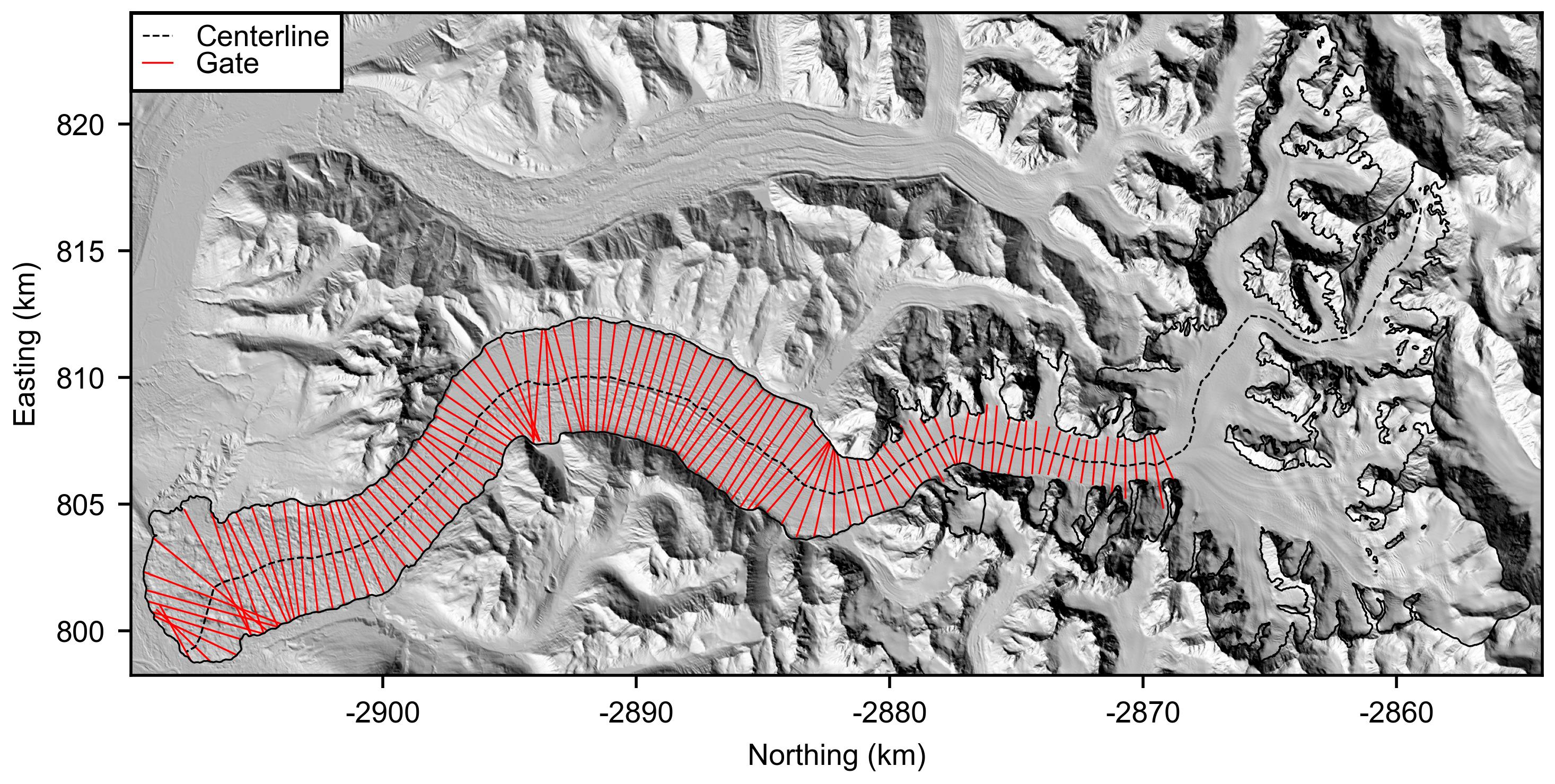
In an effort to provide detailed measurements of ice thickness for the upper Ruth Glacier, and to explore the discrepancy in ice thickness between the previous seismic survey and models, we deployed a snowmobile-towed, ice-penetrating radar system there in May 2022. We acquired nearly 150 line-km of common offset radar profiles throughout the amphitheater and gorge of Ruth Glacier. While the radar survey was successful in mapping the glacier's bed within the amphitheater, due to its geometry the gorge proved a more challenging target. To estimate the glacier's thickness therein, we combined thickness measurements provided by our surface-based survey and those from OIB-AK with surface velocities in a mass conservation approach. By constraining the ice flux between two transects (‘gates’) within the glacier's ablation zone, we find a distribution of surface mass balance parameterizations which conserve mass across our model domain. We invert for the bed position and arrive at a distribution of ice thickness solutions, from which we are able to provide a robust estimate of the depth of the Great Gorge.
2. Materials and methods
2.1. Ice-penetrating radar
2.1.1. Arizona Radio Echo Sounder
The Arizona Radio Echo Sounder (ARES) is an airborne linear-frequency-modulated radar system with a resistively loaded, end-fed towed-wire antenna that was employed by OIB-AK between 2015 and 2021 to measure the thickness of glaciers across Alaska (MacGregor and others, Reference MacGregor2021). Over 200 line-km of radar sounding data were acquired by ARES over Ruth Glacier in May 2016 and September 2019 by transmitting a waveform generated at a center frequency of 2.5 and 5 MHz, with a bandwidth of 100% relative to the center frequency (Holt and others, Reference Holt, Truffer, Larsen, Christoffersen and Tober2021). Following pulse-compression, the theoretical vertical resolution of ARES in ice is 34 and 17 m at 2.5 and 5 MHz, respectively. Clutter simulations were generated for each airborne radar profile to verify that any suspected bed returns were not generated from off-nadir surface topography (Holt and others, Reference Holt, Peters, Kempf, Morse and Blankenship2006).
2.1.2. Groundhog radar
Developed at the University of Arizona, Groundhog is a snowmobile-towed, ice-penetrating radar. On the transmit end, Groundhog employs a Kentech impulse generator which is operated at a pulse repetition rate of either 1 or 5 kHz. An Ettus X310 software defined radio was used to digitize radar echoes at 20 MHz. The transmitter and receiver were each mounted within sleds at the center of two resistively loaded 50 m half-dipole antennas. The transmit and receive assemblies are separated by ~15 m, making the total system ~215 m in length (Fig. 2). Each antenna element is encased within hollow braid polyethylene rope such that the rope, and not the resistively loaded antenna element, takes on the brunt of the tension when the system is in tow. To record system positioning information, both the transmit and receive sled were instrumented with Emlid Reach RS2+ GNSS receivers logging at 1 s intervals. Kinematic precise point positioning solutions were generated through the Canadian Spatial Reference System Precise Point Positioning web service (Tétreault and others, Reference Tétreault, Kouba, Héroux and Legree2005), resulting in positioning accurate to the decimeter level.

Figure 2. Groundhog ice-penetrating radar common-offset setup. The receiver (rx) and transmitter (tx) each sat in sleds (red) with Emlid GNSS receivers and were connected to two half-wavelength dipole antenna elements, each measuring 50 m.
Data acquisition was controlled by an operator riding within the receiver sled. Groundhog was towed across the amphitheater and the Great Gorge of Ruth Glacier between 1st May and 9th May 2022, acquiring a total of 143 line-km of common offset radar profile data. We also acquired several profiles by leaving the transmitter stationary and conducting a moveout survey. None of these provided useful data, so they will not be discussed here.
Groundhog data were uniformly processed by removing the mean trace from each profile and applying a 500 kHz–9 MHz bandpass filter. Data were migrated following the Stolt method with an assumed wavespeed in ice of 169 m μs−1 (Stolt, Reference Stolt1978), collapsing diffractions and repositioning dipping reflectors to their true subsurface locations. Profiles were vertically shifted along the fast-time axis to account for the delay between the time of transmission and the airwave-triggered start of each record.
2.1.3. Radar-derived ice thickness and bed elevation
Both ARES and Groundhog data were investigated for the presence of glacier bed returns using the open-source Radar Analysis Graphical Utility software (RAGU; Tober and Christoffersen, Reference Tober and Christoffersen2020). Horizontally continuous and high-amplitude radar returns were interpreted as echoes from the glacier bed (following verification through clutter simulations for airborne data; see Section 2.1.1). We manually digitize (‘pick’) the arrival time of the glacier bed return in ARES and Groundhog data (Figs 3, 4). In ARES data, which has been pulse-compressed to contain approximately zero-phase wavelets, this corresponds to the peak of the return, while in Groundhog data, which contain minimum phase (impulse) wavelets, this is the ‘first-break’ (onset of the first arrival; Wilson, Reference Wilson2021). Digitized bed returns provide point measurements of the two-way travel time to the glacier bed.

Figure 3. ARES example radar profile. (a) Profile A–A′ location over the lowermost ~20 km of Ruth Glacier. Context of (a) shown by red box atop white RGI glacier outline at upper right. (b) ARES radar sounding profile A–A′. Top panel shows uninterpreted profile, second panel shows clutter simulation, third panel shows interpreted profile with altimetry-derived surface elevation in blue and manually digitized glacier bed in orange, and bottom panel shows cross-sectional elevation profile with the glacier surface in blue and the bed in orange.

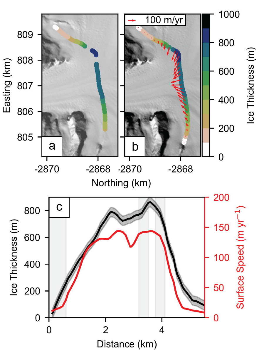
Figure 4. Groundhog example radar profile. (a) Profile B–B′ location in the Don Sheldon Amphitheater. Context of (a) shown by red box atop white RGI glacier outline at upper right. (b) Groundhog radar sounding profile B–B′. Top panel shows uninterpreted profile, second panel shows interpreted profile with the manually digitized glacier bed in orange and bottom panel shows cross-sectional elevation profile with the glacier surface in blue and the bed in orange.
Point-measurement spacing along radar profiles is a function of the radar pulse repetition rate (1–5 kHz), the system groundspeed, and the trace stacking interval, and is typically ~5 m for both ARES and Groundhog data. Following Armstrong and others (Reference Armstrong2022), the two-way travel time in ice t for a given bed return is converted to ice depth h:

where v = 169 m μs−1 is the radio wave speed in temperate ice (relative permittivity of 3.15; Evans, Reference Evans1965), c = 300 m μs−1 is the approximate radio wave speed in air, and x sep is the separation distance between the centers of the receiver and transmitter antenna elements. The transmitter–receiver separation distance for Groundhog data ranged from 105 to 120 m during the survey, varying as a function of antenna stretching and the system meandering across the surface. We use the precise separation distance provided by post-processed transmitter and receiver sled GNSS positions to calculate the depths of digitized bed returns along a given profile using Eqn (1). The midpoint between the transmit and receive sleds was assigned as the ground positioning for digitized Groundhog bed returns. ARES uses a single end-fed antenna, so the antenna separation distance x sep in Eqn (1) is zero. Accounting for the radio wave travel time from the aircraft to the glacier surface using coincident OIB-AK laser altimetry data (Larsen, Reference Larsen2020), the ice thickness is

where z is the flight altitude above ground level.
The quantization interval of bed echo interpretations, as well as the radar system timing and positioning together impact the precision of bed echo interpretations. Following Lapazaran and others (Reference Lapazaran, Otero, Martín-Español and Navarro2016), we assess the combined effect of these factors by analyzing the disagreement in ice thickness at profile intersections. Tober and others (Reference Tober2023) demonstrated from extensive crossover analysis that the precision of radar-derived bed returns for OIB-AK airborne radar data is on the order of ~10 m. We similarly assess the precision of Groundhog radar-derived ice thickness measurements in Section 3.1. Laboratory analyses have demonstrated that the dielectric permittivity in temperate ice can range from 3.1 to 3.2 (Evans, Reference Evans1965), translating to wavespeed range of 168–170 m μs−1. We therefore acknowledge an additional uncertainty in the computed ice thickness of 2%.
2.2. Estimating depth of the Great Gorge
As radar-derived measurements of ice thickness were not achievable within the Great Gorge via airborne or surface-based surveys due to the glacier's geometry (Section 4.2), we employed a mass conservation approach to estimate the glacier's thickness using radar-derived measurements of ice thickness combined with satellite-derived glacier surface velocities. Following the principle of mass conservation, the climatic-basal mass balance rate $\dot{b}$ is balanced by the ice flux divergence $\nabla \cdot \vec{q}\;$
 and the resulting change in surface elevation ∂h/∂t:

The climatic-basal mass balance rate is typically dominated by, and can thus be replaced with, the surface mass balance rate $\dot{b}_{{\rm sfc}}$ (Cuffey and Paterson, Reference Cuffey and Paterson2010), which in contrast to the climatic-basal balance rate is possible to determine through traditional field measurements.
Applying Gauss's theorem and integrating Eqn (3) across the surface area S between two transverse profiles (‘gates’), we arrive at

where q in is the ice influx from the up-glacier gate, and q out is the ice efflux from the down-glacier gate.
We calculate the ice flux q through segment (dx, dy) of a given gate as

where between consecutive points $\bar{h}$ is the average ice thickness dx is the x-distance, dy is the y-distance, $\overline {vx}$
 is the average x-component of the surface velocity, $\overline {vy}$
 is the average y-component of the surface velocity, and γ is the factor relating the observable surface velocity to the depth-averaged ice velocity.
For a glacier under simple shear with no sliding, it can be shown that γ = (n + 1)/(n + 2), where n is the exponent in the flow law of ice (e.g. Cuffey and Paterson, Reference Cuffey and Paterson2010). For the commonly used flow law exponent of n = 3, this would result in γ = 0.8. This should be seen as a minimum estimate, since a temperate glacier such as the Ruth is expected to have a significant component of basal sliding and γ is more realistically expected to fall between 0.9 and 1 (e.g. Cuffey and Paterson, Reference Cuffey and Paterson2010). Given a sensible value for γ, summing the ice flux through each segment from Eqn (5), we arrive at the total flux through a given gate.
The glacier's mean 1985–2018 surface velocity field was generated using auto-RIFT (Gardner and others, Reference Gardner2018) and provided by the NASA MEaSUREs ITS_LIVE project (Gardner and others, Reference Gardner, Fahnestock and Scambos2023; hereafter referred to as ITS_LIVE). Ice thickness data provided by the Groundhog ice-penetrating radar across the amphitheater were extrapolated to the valley edges and combined with ITS_LIVE surface velocities to constrain the ice influx to the Great Gorge (Fig. S1). To constrain the ice flux down-glacier, we take measurements of ice thickness provided by ARES ~17–20 km up-glacier from the terminus, along a profile which follows the glacier's flow direction and construct a flux gate perpendicular to ice flow. Surface speeds through this gate indicated the potential for an asymmetric cross-sectional bed shape, so we estimate the ice flux there by considering both a symmetric (parabolic) and an asymmetric bed (Fig. S2). Although another set of ARES ice thickness measurements were obtained between ~4 and 11 km up-glacier from the terminus (Fig. 1), these measurements are from debris-covered ice and are therefore less useful in constraining the surface mass balance rate.
Provided the average annual change in surface elevation for the period from 2000 to 2019 by Hugonnet and others (Reference Hugonnet2021; Fig. S3), and with the ice thickness constrained across two flux gates, the only unknown variables remaining in Eqns (4) and (5) are the surface mass balance rate and the γ-factor.
We assume that the surface mass balance rate increases linearly with altitude (e.g. Beusekom and others, Reference Beusekom, O'Nell, March, Sass and Cox2010), and can thus be expressed as

where z sfc is the surface elevation provided by a 2012 Interferometric Synthetic Aperture Radar (IFSAR) DEM, z ela is the equilibrium line altitude where the surface mass balance rate is zero, ρ ice is the density of ice, and ${\rm d}\dot{b}_{{\rm sfc}}/{\rm d}z$ is the surface mass balance gradient.
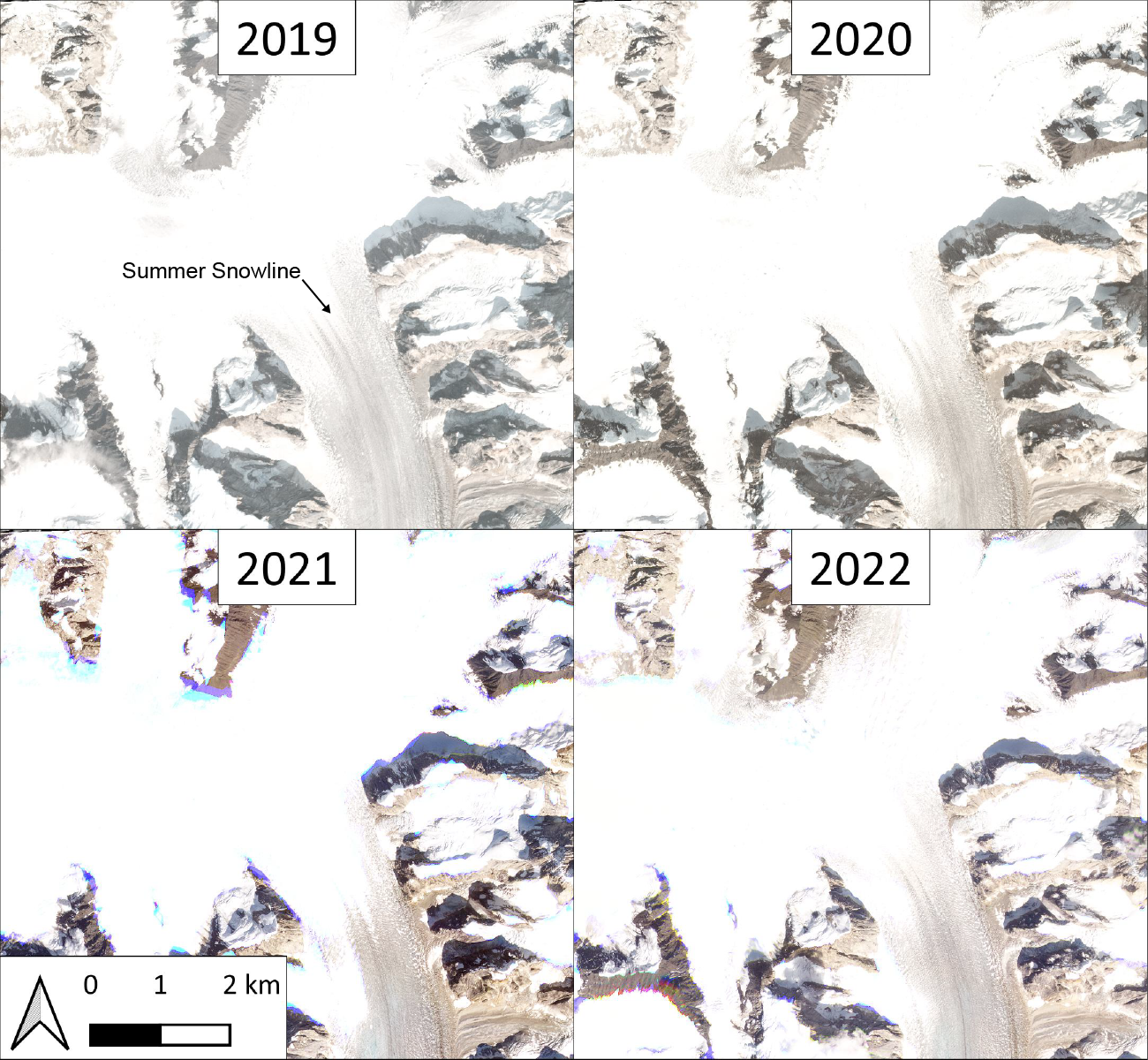
While no known records of surface mass balance exist for Ruth Glacier within the published literature, measurements for Gulkana Glacier – one of five USGS benchmark glaciers in Alaska – date back to 1966 (March and O'Neel, Reference March and O'Neel2011). Gulkana Glacier is located on the southern flank of the eastern Alaska Range, at a latitude and continental climatic setting similar to that of Ruth Glacier. While we estimate the equilibrium line altitude for Ruth Glacier based on of summer snowlines observations to be 1500–1550 m (Fig. S4) – 200–300 higher than that reported by March and O'Neel (Reference March and O'Neel2011) for Gulkana – we suspect that the annual mass-balance gradients of both glaciers are comparable. Applying a piecewise-linear fit to the annual point balance data reported by O'Neel and others (Reference O'Neel2019, their Fig. 3) provides a surface mass balance gradient of ~10 mm w.e. m−1 a−1 within the glacier's ablation zone, which we use as a reference point for the expected surface mass balance gradient of Ruth.
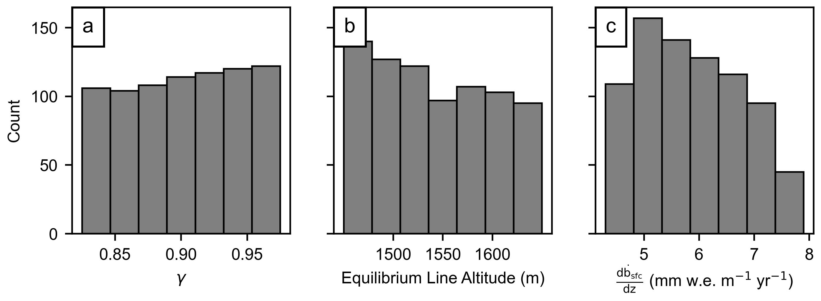
In common with many inverse problems in glaciology (e.g. Brinkerhoff and others, Reference Brinkerhoff, Aschwanden and Truffer2016; Rounce and others, Reference Rounce2020), we would expect that our mass conservation model is overparameterized: despite having some a priori information on the expected range of our unknown model parameters (γ, z ela, ${\rm d}\dot{b}_{{\rm sfc}}/{\rm d}z$ ), an infinite number of parameter combinations will likely conserve mass between our two radar-constrained flux gates. To locate all sensible parameter combinations, we perform a grid search and calculate the model misfit at our downstream flux gate relative to the median ice flux estimated through the gate from OIB-AK radar-derived ice thickness measurements, considering both a symmetric and asymmetric bed shape (Table 1). While we expect Ruth Glacier to have a significant component of basal sliding, we consider all sliding cases between 0.825 and 0.975 (0.025 step size), given that a γ-factor of 0.8 would indicate no sliding, and a value of 1 would indicate a fully decoupled glacier bed and thus ‘plug-like’ flow (Nye, Reference Nye1951). While we estimate the equilibrium line altitude to be ~1550 m based on summer snowline observations, we consider all values between 1450 and 1650 m in our grid search (5 m step size). All surface mass balance gradients between 1 and 15 mm w.e. m−1 a−1 (1 mm w.e. m−1 a−1 step size) are considered, encapsulating the reference value of 10 mm w.e. m−1 a−1 found at Gulkana Glacier by O'Neel and others (Reference O'Neel2019). We calculate the ice flux at the down-glacier extent of the model domain for all parameter permutations and consider all parameter sets which lead to a relative ice flux error of <10% as sensible (Fig. 5). A misfit threshold of 10% relative to the median value constrained by OIB-AK ice-penetrating radar was chosen such that both end-member ice fluxes for a symmetric and asymmetric bed were captured along with some margin of uncertainty. Additional analysis was performed to assess the resulting discrepancy in modeled ice thickness for a greater misfit threshold (Section 3.2).
Table 1. Mass conservation model grid search a priori estimates


Figure 5. Mass conservation model a priori parameter value grid search. Each panel (a–g) represents a different γ-factor, indicated at the lower left. Contours show the misfit in the modeled ice flux at the down-glacier extent of our model domain, relative to the ice flux estimated there by OIB-AK radar-derived ice thickness measurements. Only relative misfits less than a factor of 0.5 are shown.
For each sensible parameter set, we take the ice thickness at our upstream flux gate, the surface mass balance rate, and the ITS_LIVE surface velocity, and calculate the ice flux across a series of transects provided by the Open Global Glacier Model (OGGM; Maussion and others, Reference Maussion2019) between our up-glacier and down-glacier radar-constrained gates (Fig. S5). Assuming a parabolic glacier cross section for each gate (Nye, Reference Nye1965), we then invert for the bed position while imposing the constraint that the thickness reaches zero at the edges of each gate. Ice thickness along each gate is determined by subtracting the inverted bed position from the 2012 surface elevations provided by IFSAR. Bed elevation and ice thickness across the model domain were linearly interpolated at a spatial resolution of 100 m to provide gridded results. This inversion approach yields a mean ice thickness as well as a marginal standard deviation. We choose to present two times the marginal standard deviation as our model uncertainty, which implies an ~95% probability that the true ice thickness lies within these bounds.
3. Results
3.1. Radar mapping of Ruth Glacier
Airborne radar sounding data were acquired by ARES, primarily along centerline profiles spanning nearly the entire extent of the glacier, in both May 2016 and September 2019 during OIB-AK campaigns (Fig. 1; Holt and others, Reference Holt, Truffer, Larsen, Christoffersen and Tober2021). Per mission objectives, as OIB-AK surveys prioritized the acquisition of surface elevation measurements, aircraft trajectory was not always optimized for successful radar sounding. Investigation of ARES data revealed 10 km of glacier bed returns within the lowermost 20 km of the glacier. ARES radar-derived ice thicknesses range from ~150 to 530 m.
Nearly 150 line-km of common offset radar sounding profile data were acquired across Ruth Glacier in early May 2022 with the Groundhog radar system. Bed returns were observed and picked for 43 line-km within the amphitheater, providing point measurements of ice thickness and bed elevation along these profiles (Fig. 1). Computed ice thickness within the amphitheater ranges from ~50 to 950 m, reaching a maximum near the center of the amphitheater at the confluence of the glacier's major east and west tributary forks. Radar profiles reveal a similar geometry for both the east and west fork, with thickness reaching a local maximum of ~650–800 m at the center of each ~2.5 km-wide valley before they merge and enter the Great Gorge (Fig. 1).
Following uncertainty in the assumed wavespeed, the corresponding 2% ice thickness uncertainty gives a median and maximum ice thickness uncertainty of 8 and 10 m, respectively, for the ARES radar-derived measurements presented herein. Although sufficient data for crossover analysis were not available over Ruth Glacier, ARES crossover analysis performed by Tober and others (Reference Tober2023) over Malaspina Glacier revealed a median and interquartile range disagreement of 8 and 12 m, respectively, which we thus take to represent the precision of ARES bed echo interpretations presented herein for Ruth Glacier.
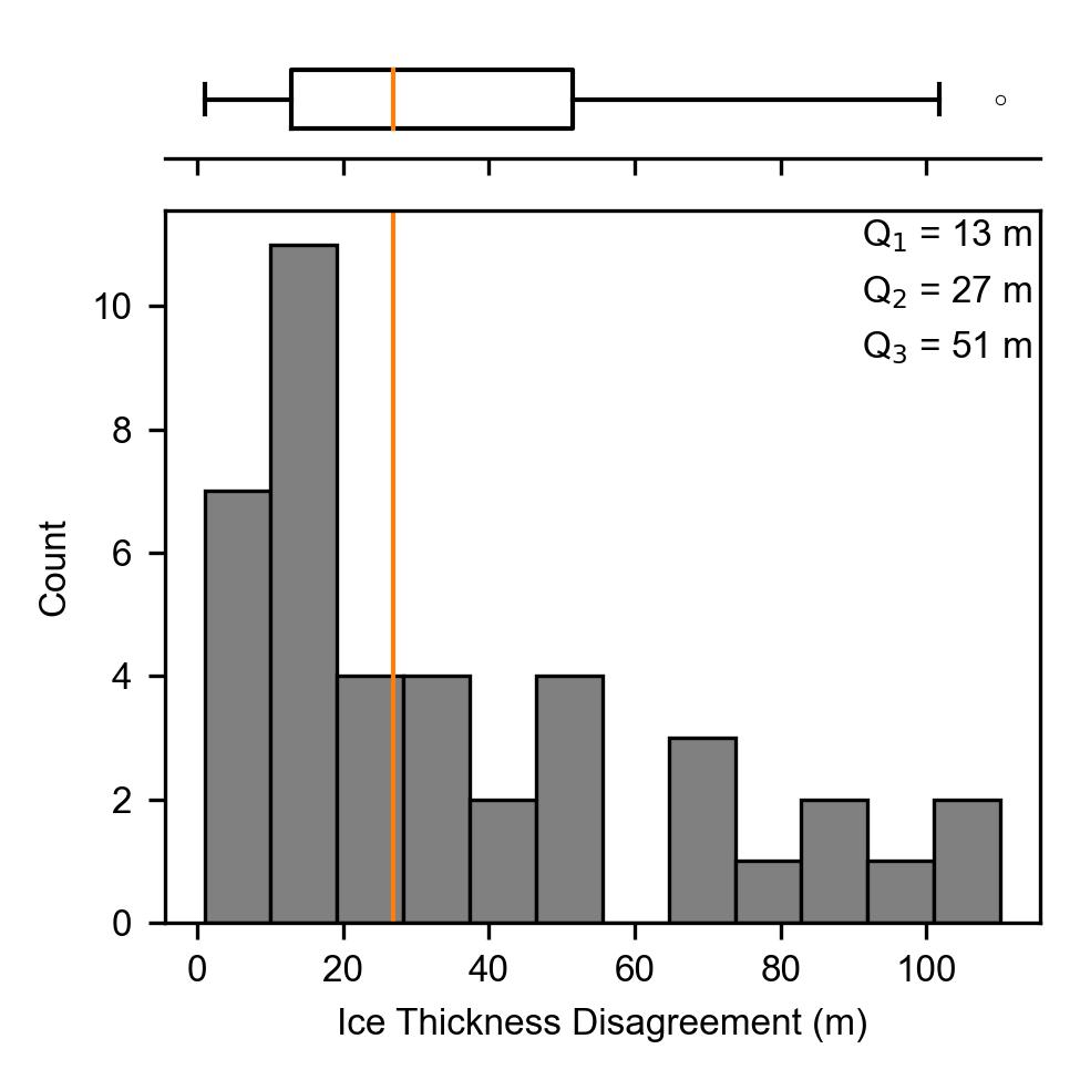
For Groundhog, uncertainty in the assumed wavespeed gives a median and maximum ice thickness uncertainty of 7 and 15 m, respectively. We assess the interpretation precision of Groundhog data by analyzing the disagreement in the computed ice thickness at 41 radar profiles which crossed paths at an angle ≥30$^\circ$ , finding a median and interquartile range difference of 27 and 39 m, respectively (Fig. S6).
3.2. Derived depth of the Great Gorge
While ~50 line-km of common offset radar profiles were acquired in the Great Gorge, no discernible bed returns were interpretable from these data. Previous researchers experienced a similarly thwarted ice-penetrating radar survey over this stretch of the glacier in the 1990s (Washburn, Reference Washburn1993). As the glacier's bed was successfully mapped throughout the amphitheater and along a stretch of the lower glacier, we sought to constrain the ice thickness in the Great Gorge through mass conservation.
Combining Groundhog radar-derived ice thickness measurements across the amphitheater with ITS_LIVE surface velocities, we find a range in the ice influx to the gorge of 0.19–0.22 km3 a−1, for a range of 0.825–0.975 in the γ-factor which relates the depth-averaged velocity to the observed surface velocity (0.21 km3 a−1 for a γ-factor of 0.9; Table S1). Approximately 28 km down-glacier, for the same γ-factor range, considering both a symmetric and asymmetric parabolic bed shape for a gate constructed perpendicular to down-glacier bed depth measurements provided by ARES, we find an ice flux range between 0.05 and 0.08 km3 a−1 (0.06–0.07 km3 a−1 for a γ-factor of 0.9). The 2000–19 average rate of surface elevation change from Hugonnet and others (Reference Hugonnet2021) for the 110 km2 between these radar-derived flux gates is −1.2 ± 0.6 m a−1 (Fig. S3). Conservation of mass then demands a specific surface mass balance rate across this stretch of the glacier between −2.1 and −2.3 m w.e. a−1, for a γ-factor range between 0.825 and 0.975.
Following our mass conservation model grid search, we find 791 parameter sets which provide a model misfit of <10% relative to our median down-glacier flux estimate (Figs 5, S7). Considering a range of 0.825–0.975 for the γ-factor, and 1450–1650 m for the equilibrium line altitude, we find that the surface mass balance gradient must be between 4.3 and 7.9 mm w.e. m−1 a−1. For all sensible parameter sets, we invert for the bed position across our model domain assuming a parabolic bed shape across each OGGM-provided transect (Fig. S5). Subtracting the inverted bed position from the 2012 IFSAR surface elevations provides a distribution of ice thickness solutions.
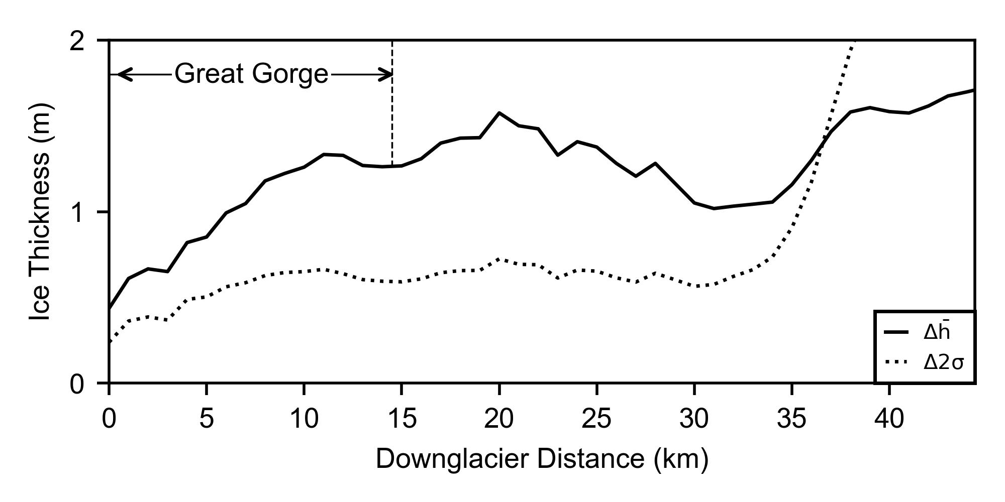
Taking the mean thickness from our distribution, we find a range of ice thickness between 610 and 960 m along the glacier's centerline within the Great Gorge (median value of 860 m; Figs 6, 7). Our model uncertainty along the centerline within the gorge ranges from 30 to 115 m. We find that the centerline ice thickness increases from 550 to 880 m within 5 km from the exit of the gorge, following a notable decrease in surface velocity from ~300 to ~100 m a−1. Bed elevation in the gorge along the glacier's centerline ranges from 240 to 740 m in reference to the WGS84 ellipsoid, and reaches a minimum value of −100 m approximately 7 km from the exit of the gorge (Figs 6d, 7). While we choose to present results for all model parameter sets which provided a relative misfit of <10%, we compare with results for a relative misfit of <25% (791 compared to 2011 permutations, respectively) and find a difference in the mean thickness and 95% confidence intervals of <2 m across our model domain (Fig. S8).

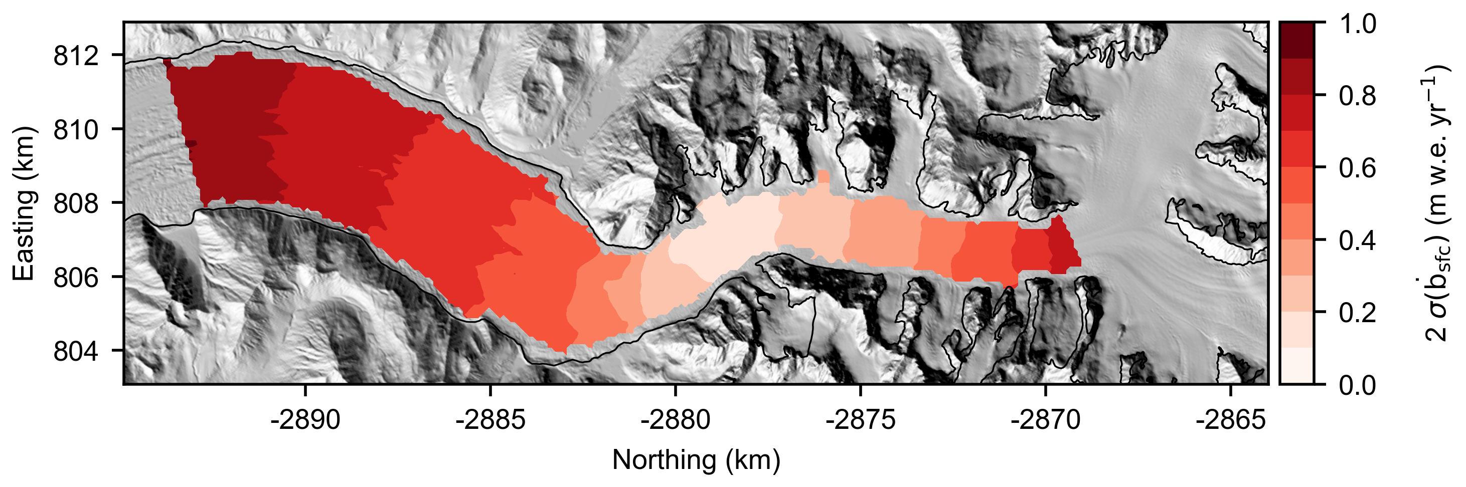
Figure 6. Flux gate mass conservation model results. (a) ITS_LIVE mean 1985–2018 glacier surface speed. (b) Mean modeled surface mass balance rate across model domain. (c) Estimated ice thickness across the model domain, provided by subtracting the mean bed solution from 2012 IFSAR surface elevations. (d) Mean bed elevation solution across the model domain. (e) 2σ model uncertainty. All panels are shown in N. Polar Stereographic projection, hence north is to the right. General ice flow direction shown at lower left corner of panel (a). Gridded model results in panels (b–e) are clipped to the extent of our down-glacier flux constraint, beyond which we have no confidence in our model results. In panels (c–e) dotted lines in the amphitheater indicate Groundhog radar measurements of ice thickness, while dashed line at down-glacier extent of the model domain indicates ARES radar measurements of ice thickness.

Figure 7. Glacier centerline geometry beginning at the entrance to the Great Gorge. IFSAR glacier surface elevation shown by blue line, and mean centerline bed solution shown by black line. 1σ and 2σ confidence intervals are shown by dark gray and light gray shaded regions, respectively. Mean bed solution shown by a dashed black line and confidence intervals have no fill beyond the down-glacier extent to which we have confidence in our mass conservation model. Red line indicates OIB-AK radar-derived bed position. While difficult to observe at the scale of this cross section, ±20 m measurement confidence interval shown by red shaded regions. Down-glacier distance represents distance from our up-glacier, radar-constrained flux gate. Maximum down-glacier extent of plot represents the glacier's terminus from version 6 of the Randolph Glacier Inventory (RGI Consortium, 2017).
4. Discussion
4.1. Comparison with previous thickness estimates
Ice thickness within the Great Gorge was derived following a grid search which was used to find all model parameter sets which upheld conservation of mass across our model domain. From the mean of our resulting ice thickness distribution we report a range in the centerline ice thickness between 610 and 960 m in the Great Gorge, with a corresponding uncertainty ranging from 30 to 115 m.
In the region of the gorge where a previous seismic reflection study proposed a depth in excess of 1 km (Echelmeyer, unpublished; Washburn, Reference Washburn1993), our mean modeled ice thickness ranges from 800 to 900 m. Nonetheless, the ice thicknesses presented within the gorge in this study are 200–600 m greater than those presented by Millan and others (Reference Millan, Mouginot, Rabatel and Morlighem2022) in their global modeling effort (Fig. 8), attesting to the remaining need for direct constraints of ice thickness and flux through ice-penetrating radar surveys. The total depth for a transect from the summit of Moose's Tooth across the Great Gorge is 2465 ± 65 m (local modeled ice thickness of 800 ± 65 m; Fig. 9), roughly matching or slightly exceeding the 2412 m-deep Hells Canyon, which currently stands as North America's deepest gorge. It is worth noting, however, that the distance from the peaks on either side of the gorge is ~5 km, while that distance is over 25 km for Hells Canyon.

Figure 8. Ruth Glacier ice thickness model comparison. (a) Modeled ice thickness from this study, as shown in Figure 6c. (b) Modeled ice thickness from Millan and others (Reference Millan, Mouginot, Rabatel and Morlighem2022). (c) Ice thickness difference between (a) and (b). Blue colors indicate a greater local ice thickness estimate from this study than that of Millan and others (Reference Millan, Mouginot, Rabatel and Morlighem2022), while red colors indicate a lower estimate.

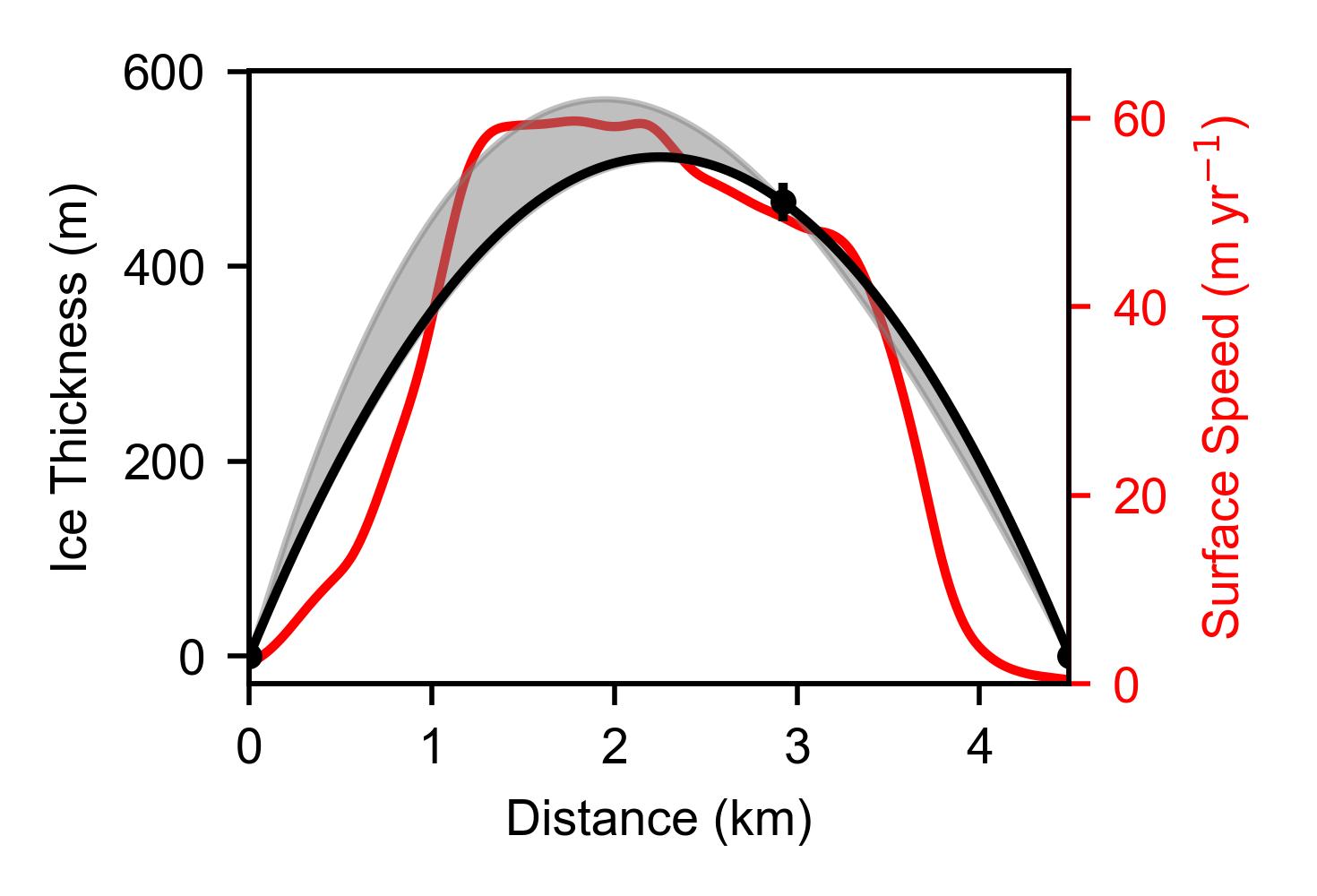
Figure 9. Great Gorge cross-sectional geometry. (a) Map view showing profile C–C′ location in red. (b) Cross-sectional profile C–C′ with glacier bed depth modeled through mass conservation in gray. Shaded gray region is the associated 2σ confidence interval.
4.2. Gorge geometry and challenges posed to geophysical surveying
We suspect that the gorge's geometry is the main cause of foiled efforts to measure the ice thickness with ice-penetrating radar. For airborne sounders such as ARES, off-nadir radar surface returns from the steep valley walls which flank the gorge prohibit successful radar bed mapping (Holt and others, Reference Holt, Peters, Kempf, Morse and Blankenship2006). Surface-based sounders such as Groundhog may experience a similar issue due to off-nadir subglacial bed returns.
In modeling radar returns for surface-based radar profiles acquired in the along-flow direction within the gorge assuming an isotropic antenna radiation pattern, we find that radar first returns would originate from off-nadir (Fig. 10), likely obscuring any potential nadir returns and therefore preventing bed mapping efforts, since it is relatively uncommon that multiple returns can be identified. At a location 1.5 km down-glacier from the entrance to the gorge, where our mass conservation-based estimate for the glacier thickness is 930 ± 90 m, this assessment demonstrates that the depth at the center of the gorge would need to be ≲750 m in order for nadir returns to precede off-nadir returns (Fig. 10). Additionally, most nadir observations of the glacier's bed in the gorge occur at high incidence angles and reflect much less power back to the radar than normal incidence off-nadir reflections.

Figure 10. Modeled radar first returns for a radar traverse across the Great Gorge. (a) Cross-sectional profile from east to west, ~5 km down-glacier of the entrance to the gorge. The mean bed solution modeled through mass conservation is shown in gray, along with shaded 2σ confidence intervals. Ray paths (dashed black) connect locations along the glacier's surface to locations along the modeled bed from which radar first returns would originate (orange) for an antenna radiation pattern which is assumed to be isotropic. (b) Comparison of radar two-way travel times across the gorge, from the glacier's surface to the nadir modeled bed position (gray, with shaded 2σ confidence interval), and to the first return (orange).
From the ~40 line-km of longitudinal common-offset radar profiles acquired within the gorge, ~2 km of suspected bed returns were initially observed. However, based on the aforementioned implications of off-nadir first returns resulting from the gorge's geometry, we discount these returns as originating from the adjacent subglacial valley wall.
The true antenna radiation pattern of a radar system employing dipole antennas such as Groundhog may be better approximated as toroidal, being omnidirectional with respect to the direction perpendicular to the antenna elements. While radar profiles acquired across the gorge may therefore be expected to help alleviate the issue of off-nadir first returns, we suspect that the antenna radiation pattern is still quite broad fore-and-aft the radar system. We observed no discernible bed returns for the 5 Groundhog profiles acquired in the transverse-flow direction (Fig. 1). Thus, even in the transverse direction, off-nadir first returns from a non-directional antenna setup may still occlude detection of the nadir bed.
4.3. Mass balance and debris cover
To constrain the surface mass balance rate across our model domain, we made use of radar-derived ice thickness measurements provided by OIB-AK between 17 and 20 km up-glacier from the terminus (Section 2.2). While another set of radar-derived ice thickness measurements were obtained between 4 and 11 km from the terminus (Fig. 1), the lowermost ~15 km of the glacier are largely debris covered. Thus, we expect that the surface mass balance rate across this stretch of the glacier cannot simply be expressed as a linear function of altitude. For this reason, we considered the flux gate we constructed from OIB-AK radar-derived thickness measurements ~17–20 km from the terminus to be the down-glacier extent of our model domain where we have confidence that the surface mass balance varies linearly with altitude. We can see the effect of neglecting debris-cover beyond this point, as the ice thickness we estimate approaches zero within ~5 km down-glacier from our OIB-AK flux constraint, ~15 km up-glacier from the glacier's terminus (Fig. 7). This model result contrasts OIB-AK observations from further down-glacier, where ice thickness measurements along the lower ~11 km of the glacier range from 150 to 500 m and highlights the need to carefully consider the complex effects of debris cover (e.g. Rounce and others, Reference Rounce2021) when making mass conservation estimates. Another complication with estimating the ice thickness through mass conservation along the lower debris-covered reaches of a glacier like Ruth is that the glacier often approaches stagnation there and so the observed surface velocity products will have large relative errors.
5. Conclusions
Between the ARES and Groundhog ice-penetrating radar systems, nearly 350 line-km of radar data have been acquired across Ruth Glacier. Investigation of this dataset provides measurements of ice thickness and bed elevation for just over 50 line-km. The majority of these measurements are obtained within the amphitheater of Ruth Glacier, with no measurements obtained within the Great Gorge.
As we were unable to map the glacier's bed within the Great Gorge, ice thickness therein was estimated through mass conservation by combining radar-derived thicknesses with satellite-derived glacier surface velocities. A flux gate in the amphitheater provided by Groundhog radar-derived ice thickness measurements constrains the ice influx to the gorge to ~0.2 km3 a−1. Nearly 30 km down-glacier, ARES provides a constraint of ~0.05 km3 a−1. Following the principle of mass conservation, we find over just under 800 acceptable model parameterizations which conserve mass across the area between these flux constraints. We invert for the bed position for each of these and find a centerline ice thickness ranging from 610 to 960 m in the gorge, with an uncertainty ranging from 30 to 115 m.
For narrow and incised glacier valleys such as the Great Gorge of Ruth Glacier, ice-penetrating radar efforts may be unable to successfully measure bed depths due to the valley geometry and the resulting radar returns from off-nadir. We have demonstrated that in such cases, if thicknesses are able to be constrained along an up-glacier and down-glacier transect, they can be combined with satellite-derived surface velocities to constrain the surface mass balance between those flux gates and then estimate the glacier thickness through mass conservation. This approach can be employed to better constrain ice thickness and flux for the numerous alpine glaciers in Alaska which remain unmapped, and for which radar sounding efforts may be limited, or may prove futile due to the valley geometry.
Supplementary material
The supplementary material for this article can be found at https://doi.org/10.1017/jog.2024.53.
Data
All radar measurements of ice thickness across Ruth Glacier presented herein, as well as mass conservation-derived thickness, gridded products, and all codes used to produce these datasets and the figures accompanying this manuscript are available at University of Arizona's Research Data Repository (doi:10.25422/azu.data.21669824). IFSAR data used to produce a DEM of the study area were collected by Fugro EarthData and acquired through the Elevation Portal of the Alaska Division of Geological and Geophysical Surveys (https://elevation.alaska.gov/).
Acknowledgements
The authors appreciate the Sheldon Chalet for providing lodging and logistics to facilitate the ice-penetrating radar survey conducted across Ruth Glacier in May 2022. The Groundhog radar survey at Ruth Glacier also would not have been possible without the support of the National Park Service, Alaska. The authors are grateful to Jason Gulley for photographically documenting and assisting in our 2022 field campaign. The authors acknowledge Tyler Meng for the many methodological discussions that helped in the development of this work. The authors are also grateful for the constructive feedback provided by two anonymous reviewers. B.S.T. was funded by NASA's FINESST program, award No. 80NSSC19K1357.


 Open access