


1. Introduction
1.1. Analyzing language attitudes in their social and geographic context
In language attitude and perceptual dialectology work, linguists are often presented with the consideration of how to disambiguate language attitudes held towards geographic areas and sociodemographic groups. For instance, in an attitudinal survey, respondents may be asked to evaluate accents which are presented to them conceptually through accent labels (e.g., Bishop, Coupland & Garett, Reference Bishop, Coupland and Garrett2005; Giles, Reference Giles1970). However, accent labels can have ambiguous designations. For instance, if a respondent evaluates the accent label “London” as having low social status, we do not know if they would also evaluate any or all speakers from London in the same light and how this could be dissected by demographic factors such as ethnicity or social class. In London, like many cities, there is considerable social, demographic and linguistic heterogeneity. Accent labels cannot simultaneously or precisely designate a geographic location such as “London” as well as sociodemographic factors such as ethnicity or social class. We cannot understand what a respondent understands by the label “London.” Therefore, using accent labels presupposes respondents’ linguistic awareness of varieties (see Preston, Reference Preston1989, Reference Preston1999).
The draw-a-map task (Preston, Reference Preston1986) is a method that has long been used in perceptual dialectology tasks to probe respondents’ evaluations of different geographic areas without the ambiguous designations of accent labels. In a draw-a-map task, informants draw isoglosses on a map based on a question such as “draw a line around places where you think people’s English sounds different” (Evans, Reference Evans2013: 272). Respondents may additionally be asked to then write their attitudes towards the speech/speakers found in each of the areas they have identified (e.g., Bucholtz, Bermudez, Fung, Edwards & Vargas, Reference Bucholtz, Bermudez, Fung, Edwards and Vargas2007; Cukor-Avila, Jeon, Rector, Tiwari & Shelton, Reference Cukor-Avila, Jeon, Rector, Tiwari and Shelton2012; Drummond & Carrie, Reference Drummond and Carrie2019). Unlike attitudinal surveys in which respondents evaluate accent labels, in draw-a-map tasks, linguists do not pre-suppose respondents’ perceptions of linguistic varieties. Respondents can freely circle areas on the map which can span official boundaries. Nonetheless, if a geographic area is evaluated as, for instance, “unintelligent,” we do not know which (if not all) demographic and social groups from the area are being evaluated in this way. Moreover, conventionally, draw-a-map tasks are accompanied by the methodological problem of how to visualize and statistically analyze results. With some exceptions (e.g., Chartier Reference Chartier2020; Drummond & Carrie, Reference Drummond and Carrie2019), draw-a-map tasks are most frequently conducted on paper (e.g., Bucholtz et al., Reference Bucholtz, Bermudez, Fung, Edwards and Vargas2007; Cukor-Avila et al., Reference Cukor-Avila, Jeon, Rector, Tiwari and Shelton2012; Montgomery, Reference Montgomery2012) which leads to difficulty in building aggregate, composite maps and performing statistical analysis (Montgomery & Stoeckle, Reference Montgomery and Stoeckle2013; Preston & Howe, Reference Preston and Howe1987).
A further limitation of both draw-a-map tasks and evaluations of accent labels is that both these measures of language attitudes may be biased by self-report. Respondents may be unaware or inarticulate of their language attitudes or may refrain from reporting them. The stereotyped evaluations of an accent that a respondent reports are, most probably, not entirely aligned with the language attitudes they actually hold towards a speaker who they encounter with that accent, whether or not they are aware of this distinction.
The language attitudes held towards the speech of different sociodemographic groups can be probed with an attitudinal survey in which respondents evaluate speech stimuli (e.g., Stewart, Ryan & Giles, Reference Stewart, Ryan and Giles1985). Although respondents are unaware of the speakers’ demographic information, they may consistently negatively evaluate speakers from specific sociodemographic groups or geographic locations. However, based on this data we cannot infer the respondent’s evaluations of any geographic area. For instance, if a respondent negatively evaluates speech stimuli produced by a speaker from London, we cannot infer that this respondent holds negative opinions of what they conceptually believe to be a “London” accent. Firstly, the respondent may not consider the speaker to be from London and secondly, they may not evaluate all speakers from London in the same way which may be conditioned by sociodemographic factors (e.g., speakers’ ethnicity and/or social class).
In sum, language attitudes made towards geographic areas and sociodemographic groups may not be in perfect alignment. Indeed, recent research has demonstrated that the hierarchy of how accents in Britain are evaluated is most pronounced when respondents are evaluating accent labels and not audio stimuli (Levon, Sharma, Cardoso, Ye & Watt, Reference Levon, Sharma, Cardoso, Ye and Watt2020). Nonetheless, we are currently lacking a measure of language attitudes towards geographic areas which neither pre-suppose respondents’ awareness of linguistic varieties nor is biased by self-report. This paper tackles this challenge by using a novel and digitized method which explores language attitudes in South East England towards geographic areas. These results are then contrasted with the language attitudes held towards sociodemographic groups based on speech stimuli.
Results reveal a complex interaction and imperfect mapping between the evaluations of geographic areas and sociodemographic groups. For instance, whilst respondents evaluate London and the county of Essex most negatively in terms of social status and solidarity, not all speakers from these areas are negatively evaluated. Instead, speakers’ demographic data is the most important factor conditioning the variation in language attitudes. The working-class and/or ethnic minority speakers from across South East England are evaluated most negatively, which is compounded if they are from East London or Essex.
1.2. Language attitudes in South East England
The two general categories most frequently used in language attitude surveys to group respondents’ evaluations of speakers/varieties/places are social status and solidarity (Preston, Reference Preston1999; Ryan & Giles, Reference Ryan and Giles1982). For instance, Stewart et al. (Reference Stewart, Ryan and Giles1985) consider the following social status traits: intelligent, confident, successful, ambitious; and the following solidarity traits: trustworthy, sincere, kind, friendly, perceived belief similarity, social class. There is often a disjunct between language varieties which receive high social status rankings and those which receive high solidarity rankings (e.g., Stewart et al., Reference Stewart, Ryan and Giles1985). This may be in part explained by the relative levels and types of prestige held by different varieties. Whilst standard varieties hold overt prestige, non-standard varieties can hold covert prestige (Trudgill, Reference Trudgill1972). For instance, Preston (Reference Preston, Hall, Doane and Ringler1992) found that African American English (AAE) does not hold overt prestige but does hold covert prestige such that young “European-Americans” may imitate AAE in order to sound “tough,” “cool,” “casual,” and “down-to-earth”.
In Britain, much work into language attitudes has revealed that firstly, working-class or ethnic varieties do not hold overt prestige and so receive low social status judgements, but in contrast can receive relatively higher solidarity judgements (Bishop et al., Reference Bishop, Coupland and Garrett2005; Giles, Reference Giles1970). Secondly, these papers also revealed that Britain’s standard variety is evaluated by Britons, even by those aged 15 to 24, as having high social status, and, although to a lesser extent, high solidarity (termed “prestige” and “social attractiveness” respectively in this work). Through standard language ideology, there has been a long-running construction of Received Pronunciation (RP) as the “best English” in England (Agha, Reference Agha2003; Milroy, Reference Milroy2001).
As RP is a class-marked standard, we would expect RP-like features to be most dominant in the areas of South East England which are most populated by the highest socioeconomic classes: parts of London (particularly some western parts), parts of the western home counties (counties surrounding London) and in particular, the county of Surrey (see Map 1 for a map of South East England). Excluding London, Surrey, which borders wealthy South West London, has a greater Gross Disposable Household Income than anywhere else in England (Office of National Statistics, 2016). Further, several of England’s most prestigious “public schools” (elite, fee-paying schools) are found in the western home counties. For instance, Eton College is found in Berkshire whilst Charterhouse School is in Surrey and charges over £40,000 in fees for each year’s boarding and schooling. These schools are strongly associated with the social and political elite. For instance, in 2019, Boris Johnson became the 20th British prime minister to have attended Eton College, where Prince William and Prince Harry were also educated. It is well established that RP is not only most predominant in the speech of the highest social classes but is particularly associated with those who attended a public school (Agha, Reference Agha2003; Badia Barrera, Reference Badia Barrera2015). Following this, we would expect parts of London, particularly South West London, the western home counties and in particular, Surrey, to be most associated with and to have the highest prevalence of South East England’s highest socioeconomic classes and subsequently, with England’s standard language variety, RP.

Map 1. The home counties and towns of South East England.
At the opposite extreme from RP, conventionally, the most “basilectal” (Wells, Reference Wells1982: 302) linguistic variety in South East England has been Cockney, which has long been associated with the white working class in East London (Cole, Reference Cole2021; Cole & Evans, Reference Cole and Evans2020; Cole & Strycharczuk, Reference Cole and Strycharczuk2019; Fox, Reference Fox2015). A more recent variety, so-called “Estuary English,” exists as a linguistic continuum ranging from England’s class-marked standard variety, RP, to Cockney, which supposedly spans all of South East England and parallels the class system (Agha, Reference Agha2003: 265; Wells, Reference Wells1997). That is, the lower the class of a speaker in South East England, the more likely they are to use Cockney-like features. In contrast, the higher the class of a speaker, the more likely it is that they will use RP-like features.
As Cockney is a working-class variety of English, it is unsurprising that a wide range of studies have found that Cockney is poorly evaluated (Giles, Reference Giles1970; Giles & Coupland, Reference Giles and Coupland1991; Giles & Powesland Reference Giles and Powesland1975). Although Wells considers Cockney to be “overtly despised, but covertly imitated” (Reference Wells, Melchers and Johannesson1994:205), respondents typically evaluate the accent label “Cockney” poorly on both social status and, to a lesser extent, solidarity judgements (Bishop et al., Reference Bishop, Coupland and Garrett2005; Giles, Reference Giles1970). Nonetheless, the same pattern is not found when respondents are evaluating the accent label “London” which receives a moderate level of social status and receives substantially higher solidarity rankings than “Cockney” (Bishop et al., Reference Bishop, Coupland and Garrett2005). The authors suggest that the “London” label is not interpreted uniformly as it fuses “stereotypes of vernacular working-class speech with very different stereotypes linked to a busy and dynamic metropolis” (Bishop et al., Reference Bishop, Coupland and Garrett2005: 139).
Indeed, London is highly diverse and throughout the 20th century, the city, particularly East London, saw a consistent fall in the population of the white working class. The so-called “Cockney Diaspora” refers to the wide-scale relocation of East Londoners into the London peripheries and home counties. In particular, the county of Essex (bordering North East London) has been the most prolific outpost of the Cockney Diaspora (Cole, Reference Cole2021; Fox, Reference Fox2015; Watt et al. Reference Watt, Millington, Huq and Smets2014). Since the late 1990s, much of London has been gentrified by the large-scale arrival of professional, managerial, and graduate populations (Butler & Robson, Reference Butler and Robson2003). Therefore, as well as white, working class Cockneys, the label “London” may also designate the accents of middle-class professionals.
Furthermore, the “London” label may now be associated with Multicultural London English. In East London, a distinct and innovative variety of English has emerged: the multiethnolect Multicultural London English (MLE). MLE emerged as a result of high rates of immigration to London which began most notably in the 1980s and led to highly ethnically diverse, multilingual, and multidialectal communities (Cheshire, Fox, Kerswill & Torgersen, Reference Cheshire, Fox, Kerswill and Torgersen2008; Cheshire, Kerswill, Fox & Torgersen, Reference Cheshire, Kerswill, Fox and Torgersen2011). Whilst previously the border between outer East London and Essex was most strongly demarcated by social class, in modern times, it is increasingly a border of ethnicity (Butler & Hamnett, Reference Butler and Hamnett2011: 8). Although MLE includes some features of Cockney, it also has features from other languages or non-British varieties of English and is most frequent in the speech of young ethnic minority speakers in East London (Fox, Reference Fox2015; Kerswill, Torgersen & Fox, Reference Cheshire, Fox, Kerswill and Torgersen2008).
Much of the above research on language attitudes towards “London” and “Cockney” labels pre-dates the documentation of Multicultural London English. Nonetheless, several attitudinal surveys have probed British listeners’ attitudes on diverse varieties of English (using the following accent labels: “Asian” and “Afro-Caribbean” [Bishop, et al., Reference Bishop, Coupland and Garrett2005]; “Indian” and “West Indies” [Giles, Reference Giles1970]; “Indian” and “Afro Caribbean” [Levon et al., Reference Levon, Sharma, Cardoso, Ye and Watt2020]). These studies coincided in demonstrating that the accent labels designating these varieties were evaluated as having very low prestige but received somewhat more favorable social attractiveness ratings. This was especially the case for “Afro-Caribbean” accents which Bishop et al. (Reference Bishop, Coupland and Garrett2005) found to be ranked relatively highly on this measure, particularly, by those aged 15 to 24 years. The authors attributed this result to young speakers “perhaps aligning this label with black and Caribbean influences in popular culture” (Reference Bishop, Coupland and Garrett2005: 141). Extrapolating these findings, MLE—which is sometimes disparagingly referred to as “Jafaican” (“fake Jamaican”) (Kerswill, Reference Kerswill and Androutsopoulos2014)—is likely to receive very low social status ratings but relatively higher solidarity ratings. The prediction of low social status ratings is corroborated by a recent qualitative attitudinal study which found that MLE is considered to be “incorrect” and a form of “broken language” and “language decay” particularly by those who do not identify as speaking this variety (Kircher & Fox, Reference Kircher and Fox2019).
Some researchers have suggested that MLE, and not Cockney, is most prevalent in the speech of young East Londoners (Cheshire et al. Reference Cheshire, Kerswill, Fox and Torgersen2011; Fox Reference Fox2015). Nonetheless, there is evidence that Cockney linguistic features were transported to the county of Essex along with the communities who relocated in the Cockney diaspora (Cole, Reference Cole2021; Cole & Evans, Reference Cole and Evans2020; Cole & Strycharczuk, Reference Cole and Strycharczuk2019). This work suggests that traditional “Cockney” features are perhaps more prevalent in Essex than any other part of the South East, including East London. As a result, in line with the negative evaluations of Cockney reported in previous studies, we would expect that both the geographic area of Essex and speakers from Essex will be evaluated negatively on solidarity and particularly social status rankings.
2. Research questions
This paper has the following research questions:
-
1. How are different geographic areas in South East England evaluated on social status and solidarity measures?
-
2. Are there differences in how speakers are evaluated on social status and solidarity measures according to their sociodemographic and identity factors? Do the evaluations of speakers differ according to respondent group?
Research question 1 is analyzed through a novel method which explores how different geographic areas are evaluated (as explained in detail in section 3.4.1). Following the research outlined in section 1.2, I predict that East London and Essex will be the most negatively evaluated geographic areas in terms of social status, and to a lesser extent, solidarity whilst South West London and the western home counties, particularly Surrey, are most positively evaluated on these measures. Further, due to the social and linguistic heterogeneity of London, I predict that there will be a substantial overlap in how London is evaluated due to the city’s high cultural and linguistic diversity.
Research question 2 examines respondents’ evaluation of speech stimuli in relation to the demographic and identity data of both speakers and respondents. Once again, following the previously outlined research in section 1.2, I predict that ethnic minority and working-class speakers will receive lower social status evaluations than white and middle-class speakers respectively. However, the speech of ethnic minority and working-class speakers may hold covert prestige and as such may receive relatively high solidarity scores. The results of research questions 1 and 2 are compared and contrasted to analyze the potential interactions and level of alignment between how speakers and geographic areas are evaluated.
3. Methods
3.1. Procedure
223 respondents undertook a 25-minute perceptual dialectology (PD) task on computers and a 5-minute production task in which they were recorded whilst individually reading aloud a wordlist and passage. The order that respondents completed the tasks was randomized. In the PD task, based on a 10-second clip of production data for each speaker, respondents completed both an attitudinal task and a geographic identification task. The experiment was completed in the ESSEXLab facilities at the University of Essex with the support of an ESSEXLab Seedcorn grant.
The experiment was run over nine days and was divided into four rounds. Stimuli from different speakers were used in each of the four rounds. In each round, the speech stimuli used was extracted from the passage reading produced by a selection of speakers from the previous round. For instance, the speech stimuli which was evaluated by respondents in round two was extracted from passage readings produced by respondents in round one. The number of respondents and speakers in each round is shown in Table 1. In total 223 respondents completed the experiment, and each judged between 27 and 29 speakers in a randomized order. A total of 102 different speakers were evaluated across the four rounds. Of these speakers, eight were repeated across rounds to give a balanced spread of geographic home locations and/or demographic characteristics in each round.
Table 1. The number of respondents who took part in each of the four rounds and how many speakers each respondent evaluated.

In the PD task, respondents were seated at computers in partitioned booths such that they could not see the screens of other respondents. The task was completed on a program that I designed and developed in Python (Van Rossum & Drake, Reference Van Rossum and Drake2009). At the beginning of the experiment, respondents provided some basic demographic and identity data which they inputted directly into the computer program. Demographic data included information such as the respondents’ schooling type, their class, ethnicity and where they were from in South East England. Respondents’ defined their ethnicity in their own words and selected their class from a drop-down list with the choices: “lower-working,” “upper-working,” “lower-middle,” “upper-middle,” “upper”.
The identity data was collected on a 100-point slider scale in which respondents responded to the following questions:
-
1. I like my accent when I talk
-
2. I am proud of where I come from
-
3. I feel that my accent is typical of where I’m from
-
4. I feel that I speak with a South East England accent
-
5. I feel that I speak with a London accent
-
6. I feel that I speak Queen’s EnglishFootnote 1
-
7. I feel I speak with a Cockney accent
-
8. I feel that I speak Estuary English
3.1.1. Language attitudes task
Based on speech stimuli, respondents made attitudinal evaluations of speakers on slider scales for the following questions:
-
1. How friendly is the speaker?
-
2. How intelligent is the speaker?
-
3. How correctly do they speak?
-
4. How trustworthy are they?
-
5. How differently do they talk from you?
Questions (1), (4) and (5) reflect solidarity judgements whilst (2) and (3) are social status judgements. Question (5) is not a clear indicator of perceived solidarity as, unlike questions (1) and (2), it is likely biased by how similar respondents actually were to speakers (e.g., for factors such as geographic provenance, age, gender, social class, ethnicity). In addition, although not analyzed as part of this present study, respondents were asked to identify speakers’ social class.
Respondents were instructed “Please move the following sliders to reflect your intuitions about the speaker. Remember that this is completely anonymous. Please provide your gut instinct.” The sliders each operated on a 100-point scale. Respondents were not made aware of this and instead, the scale was qualified as ranging from “not at all” to “very much.” Respondents were required to move each slider such that they had to make either a positive or negative judgement of any scale.
3.1.2. Geographic identification task
A measure of language attitudes towards geographic areas was ascertained by cross-referencing between the language attitudes task and a geographic identification task (the analysis is described in detail in section 3.4.1). In brief, the areas respondents were believed to be from was cross-referenced with how they were evaluated on social status and solidarity measures. This method provided insights into how respondents evaluated speakers they believed to be from a certain area, regardless of the speaker’s actual geographic provenance.
In the geographic identification task, respondents were presented with a map of South East England and were instructed to draw around the area(s) that they believed the speaker could be from based solely on their speech stimuli. This method differs from conventional geographic identification tasks in which respondents identify the speaker’s linguistic variety or geographic provenance using either fixed-choice labels (e.g., Coupland & Bishop, Reference Coupland and Bishop2007; Leach, Watson & Gnevsheva, Reference Leach, Watson and Gnevsheva2016) or free classification (e.g., Carrie & McKenzie, Reference Carrie and McKenzie2017; Mckenzie, Reference McKenzie2015). Using fixed-choice labels (e.g., “London,” “Essex”) pre-supposes respondents’ perceptions of linguistic variation and imposes linguistic isoglosses by splitting linguistic or social space. However, whilst free classification does not suffer from this problem, it provides an unrestricted possibility for answers which is difficult to aggregate and analyze quantitatively (see Mckenzie, Reference McKenzie2015 for an overview). The method employed in this study has overcome both these problems by allowing respondents to freely circle areas on a map.
Respondents were instructed that they could draw around more than one area if required, but that they could not circle more than a third of the map. Respondents could circle more than one place from across the region. This was an important consideration, as production studies have suggested that in the South East, linguistic features are not only distributed geographically, but also by ethnicity and class. Therefore, theoretically, a respondent may presume that a speaker who they believe is white and working class could be from any number of white, working-class communities in the South East that may be geographically disparate.
Respondents could optionally receive their results only after completing the entire experiment. They were instructed that their result would reflect how accurately they performed the task as well as taking into account how small an area they circled. The purpose of this design was three-fold. Firstly, creating the experiment as a challenge incentivized trying hard and the respondents were less likely to get bored. Secondly, it discouraged respondents from simply circling names of places e.g., “Essex” or “London,” but inclined them to focus on which area the speakers were actually from, therefore, allowing isoglosses to potentially span official boundaries. Thirdly, respondents were discouraged from “hedging their bets” by circling very large areas of the map. As an example, a map produced by a respondent when identifying the geographic provenance of an individual speaker (actually from North London) is shown in Map 2.

Map 2. Example of a map drawn by a respondent when identifying the geographic provenance of a speaker.
As the amount of detail and the place names listed on the maps have been shown to be important considerations in draw-a-map tasks (Cukor-Avila et al., Reference Cukor-Avila, Jeon, Rector, Tiwari and Shelton2012), the towns/cities/villages listed on the map were selected based on population data (all have >30,000 people), not on the relative cultural prominence of the places. County names (e.g., Essex, Kent, Surrey) and boundaries were included so as to help geographically orientate the respondents. The locations written with larger text (e.g., Maidstone, Chelmsford) had >100,000 population. The map only depicts the home counties; however, respondents from the South East more broadly (e.g., West Sussex or East Sussex) were also welcomed.
3.2. Stimuli
The speech stimuli used in the first round were collected prior to the experiment. As previously mentioned, in the subsequent rounds, the speech stimuli were extracted from the production data collected in the previous round. The production data consisted of readings of a wordlist and passage (adapted from Chicken Little: Blackwood Ximenes, Shaw & Carignan, Reference Watt, Millington, Huq and Smets2017). As the linguistic variables present in audio stimuli are important considerations when designing PD tasks (Leach et al., Reference Leach, Watson and Gnevsheva2016), the speech stimuli consisted of a reading of the same sentence for each speaker. The sentence was designed to include phonetic variables that have been shown to be variable and/or meaningful in South East England (e.g., variation between MLE, Cockney, and RP in rates of th-fronting/stopping, t-glottalling, h-dropping, l-vocalization, price and mouth production). The sentence used as speech stimuli was extracted from the passage reading:
‘The sky is falling’, cried Chicken Little. His head hurt and he could feel a big painful bump on it. ‘I’d better warn the others’, and off he raced in a panicked cloud of fluff.
This passage extract took approximately 10 seconds for each speaker to read. These clips were edited in Praat (Boersma & Weenink, Reference Boersma and Weenink2020) to remove disfluencies and reduce any long pauses that may affect the respondents’ evaluations of the speakers.
3.3. Respondents and speakers
All respondents and all speakers were 18 to 33 years old and were from South East England. This was with the exception of two speakers from other regions of Britain who were included as RP controls. These speakers were from areas in the Midlands (30yr, female; 26yr, female respectively), were educated at fee-paying schools, and were identified as speakers of RP. These speakers were included to see how speakers from South East England are evaluated in comparison to RP speakers who are not from the region.
As much as possible, speakers and respondents were selected whose home locations were evenly dispersed across South East England and London (Map 4 in section 4.2 shows the exact home locations of all speakers). At least one respondent and one speaker came from each of the following counties broadly in the South East: Essex, Surrey, Hertfordshire, Kent, Bedfordshire, Buckinghamshire, Berkshire, Hampshire, Suffolk, West Sussex, Hampshire, and from the following areas of London: North, North East, East, South East, South, South West, West, North West.

Map 3. The relative frequency that geographic areas were evaluated positively (heatmaps on the left-hand side) and negatively (right-hand side). When respondents considered a speaker to come from East London or southern Essex, they also tended to make negative evaluations about the speaker. In contrast, the most positively evaluated speakers were presumed to come from South West London and the western home counties, particularly Surrey. Light green = highest intensity; dark blue = lowest intensity.

Map 4. Speakers’ home locations are colored according to, on average, how intelligent they were judged to be based solely on speech stimuli. There is much variation in how speakers from very similar geographic locations are evaluated, which is most strongly conditioned by identity and sociodemographic factors, particularly social class and ethnicity. Across South East England, working-class and/or ethnic minority speakers are the most negatively evaluated speaker groups.
For both respondents and speakers, the ethnicity variable was dichotomized into white British and those from an ethnic minority background. For instance, speakers grouped as coming from an ethnic minority background had self-identified their ethnicities in the following ways: “Asian British,” “Bengali,” “Black African,” “Black British,” “British Bangladeshi,” “Brown British,” “Mixed,” and “Srilankan British.” In contrast, speakers who were grouped as “white British” identified their ethnicity as either “White” or “white British.” This meant that speakers and respondents from many different ethnicities were grouped together as coming from an ethnic minority background. I do not wish to suggest that the evaluations made of speakers from different ethnic minority backgrounds are identical, nor that there are not meaningful distinctions between the different ethnicities in this study. However, for the purpose of this study, I seek to investigate whether white British speakers are, in general, evaluated preferentially based solely on their accent. Table 2 shows the speaker summaries by ethnicity, gender, and class.
Table 2. Summary for the 102 speakers by gender, social class and ethnicity.

A majority of the respondents and speakers were students or staff at the University of Essex. Respondents were instructed that they must be less than 34 years of age and from South East England. Respondents’ and speakers’ ages are true as of the point at which they completed the experiment between March and June 2019. Respondents and speakers were considered to be eligible if they had lived at least half of the years between the ages of three and 18 in the South East. Of the 223 respondents who completed the experiment, 29 were subsequently found to not meet the eligibility criteria and were excluded from the analysis. In each of the four rounds, 7, 10, 5 and 7 respondents were excluded respectively giving a total of 194 respondents included in the analysis. Table 3 shows the respondent summaries by ethnicity, gender, and class.
Table 3. Summary of the 194 respondents by gender, social class, and ethnicity

3.4. Analysis
3.4.1 RQ1: Social status and solidarity evaluations of geographic areas
A series of aggregate, composite heatmaps were created to show which geographic areas were most positively or most negatively evaluated on social status and solidarity judgements. When respondents were completing the geographic identification task, as they circled areas on the map, the coordinates (corresponding to the pixel position) they drew were automatically extracted and exported to csv files which were stored on the lab server. The entire range of coordinates inside the shapes drawn by each respondent were then calculated using an algorithm developed in Python. A total of 774 respondent-speaker pairings were excluded as either the respondent indicated that they may have recognized the speaker, or they did not engage with the task (e.g., writing “posh” on the map instead of circling any locations). A total of 5,246 individual respondent-speaker pairings were included in the analysis.
Heatmaps were then plotted by establishing a color scale according to the relative frequencies that each coordinate was selected. The data was interrogated by the social status and solidarity judgements made in the attitudinal tasks. Separate heatmaps were produced for the lowest and highest quartiles for each attitudinal measure. For instance, a heatmap was created showing the places speakers were judged to be from each time they were evaluated to be in the lowest quartile of intelligence (<26% perceived intelligence). This was repeated for those perceived to be in the highest quartile of intelligence (>74% perceived intelligence). This was then repeated for all other social status and solidarity measures. The resultant heatmaps allow for a visual interpretation of the areas which speakers were most frequently believed to come from if they were evaluated positively/negatively on an attitudinal measure. For instance, do we find that speakers who are frequently considered as unintelligent are regularly identified as coming from a specific geographic location regardless of the speakers’ actual home locations? As with all plots in this paper, all heatmaps were plotted using the R package ggplot2 (Wickham, Reference Wickham2016).
This method circumnavigates the ambiguous designations created by accent labels which divide social and geographic space and presuppose respondents’ awareness of distinct language varieties. Further, unlike both draw-a-map and accent labels tasks, this approach does not rely on respondents being aware and articulate of their accent prejudices or being open to reporting them. This is not to suggest that draw-a-map tasks and conventional language attitude surveys using accent labels are not without enormous merit, but this method provides an insight into an alternative facet of language attitudes.
3.4.2. RQ2: Social status and solidarity evaluations of speaker groups
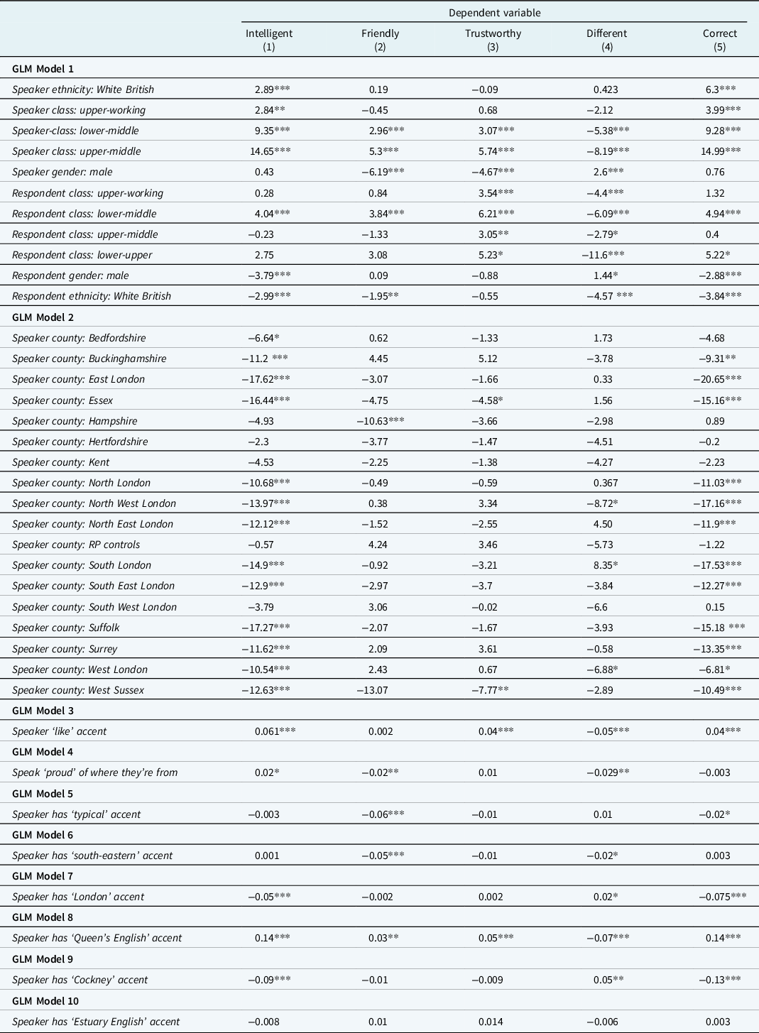
Several Gaussian generalized linear models were run in R (R Core Team, 2018). These models assessed whether, when respondents evaluate speech stimuli, there are differences in the social status and solidarity scores attributed to speakers according to their demographic and identity factors. In addition, the models assessed whether the evaluations of speakers were related to the respondents’ demographic data. Respondents evaluated speech stimuli without being provided with any prior information about the speaker. This affords an analysis of how different sociodemographic groups are evaluated based solely on their speech without requiring respondents to self-report their language attitudes. Separate analyses were run with each of the social status and solidarity scores as the dependent variable (whether the speaker is perceived as intelligent, friendly, trustworthy, speaking differently to the respondent, and as speaking correctly).
The independent variables included were related to the speakers’ demographic data: (1) speakers’ social class (self-identified from fixed choice options), (2) ethnicity of speaker (self-identified and aggregated into white British speaker/ethnic minority speaker); (3) gender of speaker; (4) home location of the speaker which was a categorical variable with 19 levels: the counties that speakers originated from (Essex, Surrey, Hertfordshire, West Sussex, Kent, Bedfordshire, Buckinghamshire, Berkshire, Hampshire, Suffolk) as well as London split into eight distinct areas (North, North East, East, South East, South, South West, West, North West) and finally the two controls who were not from any area of South East England. The reference level was set as “Berkshire” as a baseline control for comparison in the model. Following the research outlined in section 1.2, we would expect speakers from Berkshire to be evaluated positively and therefore to be at the extreme of the scale. However, unlike counties such as Surrey, the county lacks “cultural prominence” and as such, it is unlikely that respondents would have strong perceptions of what a speaker from Berkshire would sound like.
Further independent variables were included from the speakers’ identity data regarding whether the speaker felt their accent was: (5) typical of where they were from; (6) Cockney; (7) Queen’s English; (8) Estuary English; (9) a London accent. The final identity variable was (10) to what extent the speakers felt proud of where they were from. Finally, independent variables were included relating to the respondents’ demographic data: (11) the respondents’ social class (self-identified); (12) ethnicity of respondent (white British respondent/ethnic minority respondent); (13) gender of respondent. The reference level for both respondents’ and speakers’ social class was “lower-working” as the extreme of the scale.
In order to avoid multicollinearity, several different models with different predictors were run for each of the dependent variables. Firstly, predictors (1) to (3) and (11) to (13) (related to speaker and respondents’ social class, ethnicity and gender) were included in a separate model to other predictors. Secondly, models were run with only predictor (4). Predictor (4) was not included in the same analysis as speakers’ ethnicity and class as it was not independent from these two variables. For instance, 62% of speakers from an ethnic minority background in the sample came from London compared to 14% of the white British speakers.
Finally, separate models were run for each of predictors (5) to (10), relating to the speaker’s identity data as there were correlations between these factors. For instance, there was a negative correlation between a speaker considering their accent to be “Cockney” and “Queen’s English.” Separate models were run to avoid multicollinearity which could potentially reduce the predictive power and reliability of the model. Gaussian models were run as this reflected the distribution of each dependent variable which most closely resembled a normal distribution. For each analysis, significance was interpreted with α set at 0.05.
4. Results
4.1. RQ1: Social status and solidarity evaluations of geographic areas
A series of aggregate composite heatmaps (Map 3) show how positively or negatively geographic areas were evaluated on social status and solidarity judgements. For each measure, positive (>74%) and negative evaluations (<26%) are on the left-hand side and the right-hand side of Map 3 respectively. The heatmaps show that, in general, on all social status and solidarity measures, much of London, particularly South West London, as well as the western home counties (Buckinghamshire, Berkshire, Hertfordshire and particularly Surrey) were evaluated most positively. Whilst the effect was strongest for social status measures, it was also present for solidarity measures. In contrast, London (particularly East London) and Essex (particularly southern Essex) were evaluated most negatively on all measures. There is substantial overlap in how London was evaluated. For all measures, speakers who were considered by respondents as coming from London were amongst the most positively and the most negatively evaluated.
4.2. RQ2: Social status and solidarity evaluations of speaker groups
Generalized linear models found significant differences in social status and solidarity scores according to both respondents’ and speakers’ sociodemographic factors (see Table 4 in the appendix for the model outputs). In terms of the respondents’ characteristics, male respondents were found to be more negative in their evaluations of speakers (as also found by Coupland & Bishop, Reference Coupland and Bishop2007). In general, they evaluated speakers as less intelligent, speaking less correctly, and speaking more differently to themselves than women respondents did. White British respondents also tended to be more critical than respondents from an ethnic minority background. They judged speakers to be less friendly, less intelligent, and as speaking less correctly but more similarly to themselves. It may not be surprising that white British respondents, in general, perceived speakers as speaking more similarly to themselves, given that 79.4% of speakers were indeed white British (although respondents were unaware of this proportion). Compared to lower-working-class respondents, those of a higher class tended to be less critical in their evaluations of speakers. The lower-middle class were by far the most positive evaluators whilst the lower-working class were the most negative.
In terms of speakers’ demographic factors, in general, the higher a speaker’s class, the more likely they were to be evaluated positively on social status measures. For instance, as shown in Figure 1, the mean score for perceived intelligence was 50% for the lower-working class compared to 64% for the upper-middle class. In addition, the upper-middle class were judged as speaking significantly more correctly than the lower-working class (68% vs. 52%). Additionally, although the effect was not as large as for social status measures, upper-middle-class speakers were perceived as having higher solidarity compared to lower-working-class speakers. They were judged to be significantly friendlier (62% vs. 58%), more trustworthy (59% vs. 54%) and speaking more similarly to the respondent (60% vs. 52%).

Figure 1. The social class of speakers and how intelligent they were perceived to be based solely on their accent. The higher a speaker’s class, the more likely they were to be evaluated as intelligent.
In terms of ethnicity, compared to speakers from an ethnic minority background, white British speakers were evaluated as having significantly higher social status. White British speakers were judged to be more intelligent (58% vs. 53%) (Figure 2) and to speak more correctly (62% vs. 54%). There were no significant differences in solidarity ratings between ethnic minority and white British speakers.

Figure 2. The ethnicity of speakers and how intelligent they were perceived to be based solely on their accent. White British speakers were evaluated as significantly more intelligent than ethnic minority speakers.
A self-bias effect was found for both class and ethnicity. That is, both white British and ethnic minority respondents evaluated ethnic minority speakers as less intelligent and as speaking less correctly than they evaluated white British speakers. For instance, on average, ethnic minority respondents judged white British speakers to be 59% intelligent which was higher than their evaluation of other ethnic minority speakers (55% intelligent). A similar effect was found for social class (Figure 3). Those who considered themselves to be lower-working class judged the higher classes as more intelligent and as speaking more correctly. For instance, lower-working-class respondents evaluated other lower-working class speakers on average as 48.2% intelligent compared to their judgement of upper-middle class speakers as 63.3% intelligent.

Figure 3. The perceived intelligence of speakers based solely on accent in relation to the social class of both respondents and speakers. There is a self-bias effect. All classes, including the lower-working class, evaluate lower-working-class speakers as less intelligent than speakers from higher classes.
The relationship between how speakers were evaluated and their gender was more complex. Regardless of the respondent’s gender, male speakers were perceived as more intelligent (58% vs 56%) and as speaking more correctly (61% vs 59%) than female speakers (though the effect was not statistically significant for these two measures), but also as speaking less similarly to the respondent (55% vs 57%) and as being less friendly (57% vs 62%) and less trustworthy (54% vs 59%). In general, men were perceived as having more social status whilst women were perceived as having more solidarity.
There were also significant effects relating to the speakers’ identity data. Speakers who identified their own accent as “Cockney” or “London” were considered to be significantly less intelligent and as speaking less correctly and more differently to the respondent. Those who considered their accent to be “south-eastern” or who indicated they were “proud” of where they are from were evaluated as less friendly but speaking more similarly to the respondent. Speakers who indicated that they liked their accent or those who believed they spoke “Queen’s English” were evaluated most positively on all social status and solidarity measures (with the exception of perceived friendliness which was not significantly related to how much speakers liked their accents). In terms of identity factors, the greatest effect was found for “Queen’s English”. Those who considered their accent to be “Queen’s English” were evaluated as significantly more intelligent, friendly, trustworthy and as speaking more correctly and more similarly to the respondent.
There were no significant patterns between how speakers were evaluated on solidarity measures and where they were from. However, in terms of social status, compared to the reference level, speakers from the following areas were evaluated significantly more negatively on both measures (perceived intelligence and speaking correctly): Essex, East London, North West London, North East London, North London, South East London, South London, West London, as well as Buckinghamshire, Surrey, Suffolk, and West Sussex (Figure 4). As predicted then, speakers from London as well as Essex were, on the whole, amongst the most negatively evaluated speaker groups. In addition, as hypothesized, the RP controls, as well as the speakers from the western counties such as Hertfordshire, Berkshire, Bedfordshire, Hampshire were evaluated most positively, as well as speakers from South West London.

Figure 4. The home location of speakers and how they were evaluated on social status measures. Home locations are ordered from the highest mean score to the lowest for each attitudinal measure. Whilst there is much variation, in general, speakers from Essex and London are evaluated negatively whilst speakers from South West London and much of the western home counties are evaluated positively.
However, speakers from the same location were not evaluated uniformly. For instance, some speakers from East London were, on average, evaluated as speaking more correctly than the RP controls. Similarly, some speakers from Surrey were evaluated as less intelligent than the majority of speakers from East London. There was particularly high variation in how speakers from Essex were evaluated. Of all speakers in the sample, both the most positively evaluated speaker and the most negatively evaluated speaker on social status measures were from Essex (e.g., 78% vs. 23% score on perceived intelligence). The most positively evaluated speaker was from a village in northern Essex. The most negatively evaluated was from an area in southern Essex formed as part of the East London slum clearance programmes, where Cockney linguistic features are still present (Cole, Reference Cole2021).
Map 4 shows the actual home location of speakers and how positively they were evaluated. There are stark differences in how speakers from almost identical locations are evaluated. Demographic and identity factors were crucial in explaining the variation in how speakers from the same area were evaluated. To provide an example, two white female speakers from Essex lived just 1.5 miles apart. However, they received mean perceived intelligence scores of 70% and 29% respectively. The former lives in an affluent area, attended fee-paying school, is university educated, and identified as lower-middle class. The latter is from a council estate, attended state school, did not attain any further education and identified as lower-working class.
5. Discussion
This paper has investigated language attitudes amongst young people in South East England with a broader methodological aim of disambiguating language attitudes held towards sociodemographic groups and geographic locations. Results reveal that working-class and ethnic minority speakers are evaluated less positively on solidarity and particularly social status measures compared to middle-class and white British speakers respectively. Contrary to the predictions of this paper, the accents of working-class speakers in South East England do not hold covert prestige. However, there were no significant differences in how ethnic minority and white British speakers were evaluated on solidarity measures, suggesting that the accents of the former may hold some limited covert prestige.
Speakers who considered their accent to be “Queen’s English” were very positively evaluated. However, as England’s standard language is delocalized and class-marked, speakers who identified their accent with geographically marked terms such as “London,” “Cockney,” “typical,” or even those who indicated they were “proud” of where they come from, were evaluated negatively. There was also a trend for speakers from certain areas, especially London and Essex, to receive negative evaluations on social status measures, but there were no significant patterns for solidarity measures.
The results of this study corroborate previous research in which respondents’ evaluations of accent labels have revealed a remarkable consistency in the hierarchy of British accents (Bishop et al., Reference Bishop, Coupland and Garrett2005; Giles, Reference Giles1970; Levon et al., Reference Levon, Sharma, Cardoso, Ye and Watt2020). In these studies, RP (as designated through accent labels) was the most positively evaluated variety in contrast to working class and ethnic varieties which were evaluated most negatively. The self-bias effect for both ethnicity and class that was revealed in this paper demonstrates that standard language ideology operates intuitively and goes widely unchallenged even by those who it directly disadvantages. Although respondents were provided with no prior information about speakers, results demonstrated that speakers’ demographic and identity factors, particularly class and ethnicity, were crucial in determining how they were evaluated.
Effects were also found regarding how geographic areas were evaluated. The heatmaps presented in section 4.1 reveal systematic patterns in how different geographic areas are perceived. As predicted, if a speaker received a negative evaluation based on their accent, they were most frequently identified, often erroneously, as coming from East London and/or southern Essex. In contrast, the speakers who received the most positive evaluations were presumed, once again often erroneously, as originating from London and/or the western home counties, particularly South West London and Surrey. Whilst these patterns were strikingly consistent for all social status and solidarity measures, the effect was greatest for the former. These results demonstrate that, as a result of the movement of Cockney people and their dialect to Essex (Cole, Reference Cole2021, Cole & Evans, Reference Cole and Evans2020), negative evaluations of Cockney (Bishop et al., Reference Bishop, Coupland and Garrett2005; Giles, Reference Giles1970; Giles & Coupland, Reference Giles and Coupland1991; Giles & Powesland Reference Giles and Powesland1975) have now been transposed onto Essex.
Nonetheless, the heatmaps cannot be interpreted independently of respondents’ accuracy in the geographic identification task. The heatmaps depict the intersection between how speakers were evaluated and where they were thought to come from. If speakers from Essex are evaluated negatively but are consistently accurately identified as coming from Essex, the heatmaps would depict language attitudes held towards Essex speech stimuli and not necessarily towards their conception of an Essex accent. Nonetheless, in this study, speakers who were thought to be from Essex were consistently evaluated negatively, regardless of whether or not they were indeed from Essex or not. Although a detailed analysis of the geographic identification task is outside the scope of this paper, in brief, respondents performed the geographic identification task with only 12.15% accuracy (though significantly better than chance at 9.7%). Further, accurately circling a speaker’s home location is not necessarily synonymous with the respondent knowing where a speaker is from as they may have circled up to a third of the map. Thus, the heatmaps depict respondents’ stereotyped evaluations of different geographic areas and not how speakers actually from these areas were evaluated. As demonstrated, speakers from very similar locations were evaluated in remarkably disparate ways, which was strongly conditioned by demographic factors.
This effect was most notable for London. Amongst many other groups, London is home to white, working-class speakers of Cockney, ethnic minority speakers of MLE, and middle-class professionals who are most likely to speak RP-like varieties. It is not surprising that previous research has found that the accent label “London” holds ambiguous designations and is evaluated differently to the label “Cockney” (Bishop et al., Reference Bishop, Coupland and Garrett2005). Correspondingly, in this study, neither the geographic area of London nor speakers from London were evaluated uniformly. Instead, language attitudes were most strongly conditioned by speakers’ demographic, and to a much lesser extent, identity factors.
The imperfect mapping between the evaluations of geographic areas and sociodemographic groups is not to suggest that the two are not intricately related. It is no coincidence that, firstly, the most negatively evaluated geographic areas are East London and Essex and, secondly, the working class and/or ethnic minority speakers are the most negatively evaluated speaker groups. Indeed, these geographic areas are the most populated, or at least, the most associated with these sociodemographic groups. Nonetheless, the stereotyped evaluations of geographic areas only loosely translate to how speakers actually from these areas were evaluated. Whilst respondents perceive East London and Essex most negatively, not all speakers from these areas were evaluated negatively. Instead, working-class and/or ethnic minority speakers from across South East England are evaluated most negatively, which is compounded if they are from East London or Essex.
In sum, this paper has demonstrated that disambiguating the language attitudes held towards sociodemographic groups and geographic areas is paramount to understanding the configuration of language attitudes in an area, particularly, for areas which have high cultural and linguistic heterogeneity. The results have revealed systematic patterns in the stereotyped evaluations of different geographic areas which does not perfectly map onto how speakers actually from these areas are evaluated. Instead, language attitudes towards speech stimuli were most strongly conditioned by speakers’ identity and demographic factors, particularly class and ethnicity. In South East England, a hierarchy of accents pervades which disadvantages ethnic minority and/or working-class speakers, particularly those from Essex or East London, whilst it simultaneously bestows speakers of the class-marked and de-localized standard variety with more favorable evaluations.
Appendix
Table 4. Coefficient and significance values for a series of Gaussian generalized linear models assessing the effect of both speaker and respondent demographic and identity data on language attitudes. In general, based solely on their accent, working-class speakers, ethnic minority speakers, those from London or Essex, and those who define their accent with geographically marked terms receive the most negative evaluations.
Signif codes: p<0.05*; p<0.01**, p<0.001***


 Open access