


1. INTRODUCTION
Terrain Referenced Navigation (TRN) techniques determine position by performing a comparison between stored terrain Digital Elevation Maps (DEM) and data obtained from sensors. In batch processed TRN, a series of height measurements (commonly known as transect or measured profile) are processed together. Since the TRN signal is formed by separate, independent measurements, the system also requires information about the relative distance and direction between these samples. Hence, the speed and the heading of the platform need to be accurately estimated. Inertial sensors can provide this information, but they are still subject to measurement errors.
Likewise, in a Global Positioning System (GPS) receiver, the frequency and the code phase of the incoming signal are changing parameters in time and accurate estimations are needed in the decoding process. Both with GPS and TRN, uncertainty is present with respect to the spacing between received samples. Also, in both cases, the unknown shift (relative to a predefined reference) is solved by correlating a measured signal with a local replica. Previous work (Vaman and Oonincx, Reference Vaman and Oonincx2010) has been dedicated to the study of the similarities between these two apparently different navigation techniques. Based on this analysis, we explored the potential of adapting to the TRN field a series of Digital Signal Processing (DSP) techniques that have been originally developed for the acquisition and tracking of GPS signals.
A GPS based TRN algorithm has been developed in (Vaman and Oonincx, Reference Vaman and Oonincx2010) and (Vaman et al., Reference Vaman, Theunissen and Oonincx2011) and its performance is being explored, evaluated and improved through simulations. The basic rationale behind the algorithm is that navigation can be assured by continuously following changing velocities and orientation of the vehicle. Although inertial sensors provide estimates for these parameters, their values are still affected by disturbances. Data in the DEM is compared with the elevation measurements, to effectively compensate for these disturbances. Comparing terrain profiles with incoming measurements is achieved by correlation; the novelty of the algorithm consists in the estimate process of speed and heading. Further, inspired by GPS techniques, this process consists of two phases: The acquisition finds phase coarse estimates of the parameters, whereas tracking adjusts the values for fine tuning.
The C/A codes, used for GPS, do differ from terrain ‘codes’ in randomness. Due to the arbitrary character of terrain profiles, the corresponding correlator does not have a predefined shape. Its magnitude is variable and its shape may be skewed and asymmetric. Due to these issues, the early-late tracking scheme cannot be implemented in a straightforward manner.
We have been investigating whether DSP techniques used in GPS can be adapted to mitigate the shortcomings caused by the non-ideal TRN terrain signal. At first glance such an approach may seem peculiar because of the differences in signal properties. In reality however, there is no ‘ideal’ GPS signal and disturbances (such as multipath and interference) distort the shape of the correlation function, causing asymmetry and bias. Hence, GPS multipath mitigation strategies based on correlation techniques may turn out to be useful as well for effectively dealing with asymmetric TRN correlators.
The current paper focuses on the identification and evaluation of GPS multipath mitigation strategies signal processing concepts that can be adapted and embedded to the developed TRN algorithm. The paper starts with a brief description of the operating principle of the TRN tracking loop, in order to clarify to the reader the encountered challenges. Details on the entire architecture of the loop, along with other design issues can be found in (Vaman, Reference Vaman2011).
2. REVIEW OF THE PROPOSED TRACKING LOOP
Civil standard GPS signals use as spreading sequences the C/A codes, which are Pseudo Random Noise (PRN) sequences. These codes are characterized by important correlation properties: nearly no cross-correlation and nearly no correlation except for zero-lag. An example of a C/A code Auto Correlation Function (ACF) is illustrated in Figure 2a: when two identical codes are perfectly synchronized, the correlation function shows a large, distinct peak.
In order to reconstruct the navigation message data, a GPS receiver needs to determine two properties of the received signal: frequency and code phase. The code phase denotes the point in the current data block where the C/A code begins. Due to the movement of satellites (and of the receiver itself) both properties change continuously, as a function of time. Therefore, after being acquired (i.e., roughly estimated) the parameters still need to be monitored. This is the task of the tracking process. Code tracking is solved by means of the Delay-Lock Loop (DLL) scheme, based on a two-correlator structure. Each correlator is set with a small time offset relative to the promptly received signal code phase, generating early and late replicas of the code. These replicas are then correlated with the incoming signal. Given the shape of the C/A code ACF, perfect alignment (between the generated code and the received one) is considered to be found when the early and late versions have equal correlation values (Borre et al., Reference Borre, Akos, Bertelsen, Rinder and Jensen2007).
In the proposed TRN algorithm, the tracking module was implemented to monitor the changes of two parameters: the speed and the heading of the traveling vehicle. Tracking is performed sequentially, using a separate loop for each one of the above mentioned parameters. As the rationale behind the development is the same, throughout the paper we will refer to the velocity loop only. The TRN tracking loop has been designed as an early-late correlator, inspired by the DLL's functional principle. A block diagram illustrates the loop in Figure 1.

Figure 1. Diagram of the TRN tracking loop block.
The subsequent terrain measurements are grouped in an array, forming the incoming TRN signal (also referred to as measured profile). The early and late replicas are generated by extracting profiles from the database using two small offsets relative to the estimated speed. Next, correlation between these tracks and the measured profile is computed, by means of an average distance function. The error signal is formed from the combination of the correlation outputs. The early-late spacing is also considered in the computational expression, see (Vaman et al., Reference Vaman, Theunissen and Oonincx2011).
As mentioned before, terrain ‘codes’ are not deterministic sequences. Therefore, the TRN correlator does not have a predefined shape. The auto-correlation peak is distinct, but cross-correlation values have a dynamic range. An example of a TRN speed correlation function is illustrated in Figure 2b.

Figure 2. Comparison: (a) C/A code auto-correlation (left), (b) TRN velocity correlation (right).
The main differences between GPS and TRN correlation and tracking are summarized in Table 1.
Table 1. Differences between GPS and TRN signals.

Similarly to the GPS code correlation function, the TRN correlation function provides a measurement of the alignment between the signal and reference codes. This has been the premise of adapting the DLL scheme to TRN. However, given the properties of the terrain signals, the early-late approach cannot be applied in a straightforward manner. The following issues must be considered.
2.1. Assessing Convergence and Fast Convergence
The convergence requirement represents the need that the system finds ‘lock’, without entering an oscillating behaviour. With an early-late tracker it is considered that the signal is aligned with its database replica if the early and the late channels are equal and no error is generated by the discriminator. Given that the magnitudes of the TRN correlation peak and of the cross-correlation vary, the error generated in the loop will only tend towards null value. The issue can be solved by replacing the ‘null seeking’ strategy with a small threshold. The TRN loop will be considered ‘in lock’ when the difference between the early and late correlation outputs is equal to the preset threshold. The fast convergence requirement is related to the minimization of the number of iterations needed to establish lock. This depends on the disturbance value, but as a general rule a wide spacing between channels allows a better capability of rejection.
The maximum rated value for the spacing can be computed by analysing the properties of the reference signal. An early-late concept can be applied only while the correlation function is V-shaped (i.e., the difference between the two shifted replicas cannot exceed the width of the correlation peak). We refer to this as the bandwidth property. The calculation procedure has been illustrated in Figure 3 (left).

Figure 3. Bandwidth of TRN correlation functions (left) and bias from correlation symmetry (right).
2.2. Managing Error Bias
The discriminator is designed to keep the power of the early and late correlators (quasi) equal. In general, the TRN correlator is skewed and asymmetrical. A distorted correlation function will bias the process, as illustrated in Figure 3 (right).
The range of the error bias caused by the asymmetry can be estimated by analysing the correlation function of the reference signal. The mathematical relationship between the slopes of the lines that form the correlation peak, and the spacing and the range of the bias to be expected is given by:
where s1 and s2 represent the slopes of the fitted lines, left and right from the peak, corresponding to the used spacing.
The analysis is not extremely precise because it has been derived from slopes of the fitted lines. If the correlation function is formed by segments with varying slopes as in Figure 4, fitting lines through these points will result in errors. However, we can use Equation (1) as an indication for assigning the spacing. Once a threshold for the desired range of bias is set, the spacing can be calculated using this equation. The main idea is to reduce part of the error bias in a first stage, while also assessing convergence. In a second stage, mitigation strategies will be applied to further eliminate or compensate for the bias error and to refine the solution.
When dealing with the errors caused by the asymmetry of the correlation function we returned to GPS techniques. The next section discusses the investigated aspects.
3. RECEIVER INTERNAL CORRELATION TECHNIQUES FOR MINIMISING CODE MULTIPATH ERROR IN GPS
Out of the different error sources associated with GPS signal processing, multipath directly affects the code tracking process. In the case of multipath propagation, the received signal is a distorted version of the transmitted one. In addition to the direct signal, the receiver observes other replicas propagated via longer paths, due to interactions with one or more obstacles in the environment.
Reception of multipath can cause significant distortions to the shape of the correlation function. Figure 4 illustrates this effect for reflected and direct signals that are in-phase (left) and out of phase (right). We note that the effect of multipath results in a skewed and asymmetric C/A code correlator, with unequal slopes of the lines on either side of the peak. This shows similarity to the natural shape of the TRN correlator, see Figure 2b.

Figure 4. Constructive (left) and destructive (right) multipath interference.
In the past, significant work has been performed to improve the multipath rejection performance of GPS receivers. Among the wide scope of developed methods, we focused on an algorithm based receiver internal correlation techniques, which we discuss here for a potential adaptation to the TRN case.
3.1. Narrow Correlator Spacing (NCS) Technique
Historically, conventional GPS receivers have used a 1.0 chip early-late correlator spacing in the implementation of DLLs. The advantage of choosing a wide spacing was mostly related to having a wide bandwidth to better cope with disturbances. It was in the early 1990s that tracking with a much narrower spacing was investigated. The results showed important reduction of tracking errors in the presence of both noise and multipath, especially in C/A code applications. This happens because the distortion of the cross-correlation function near its peak is less severe than in the regions away from the peak. Therefore, if tracking can be performed in the peak area, the effects of multipath will be considerably reduced. This is a statement applicable mostly to the non-coherent DLL versions. For a coherent DLL this observation is not true under conditions of strong multipath reception, due to the susceptibility to carrier phase tracking errors (Van Dierendonck et al., Reference Van Dierendonck, Fenton and Ford1992).
3.1.1. Possible Adaptation to the TRN Case
The TRN correlation function is also less distorted in the peak area. This is a consequence of working with terrain signals: adjacent elevation samples are more correlated between each other than distant ones. It is expected that the correlation function will be symmetrical around the peak. Therefore, by performing tracking with a narrow spacing, the effects of asymmetry should be reduced. When adapting and testing this strategy to the TRN algorithm, there are two main questions to be answered, namely: which spacing values would form the set of inputs and what should be the boundaries of this interval?
3.1.2. Implementation
As previously discussed, the first step in TRN tracking is assessing convergence. During this process, the spacing is selected based on the analysis of the bandwidth and the symmetry properties. The numerical value chosen at that stage represents the upper limit (the maximum spacing) for applying the Narrow Correlator Spacing (NCS) technique. Theoretically, there is no lower limit to it. Early and late profiles can be extracted from the database by using infinitesimal offsets relative to the estimated speed. In practice, it depends on the resolution of the database, the speed at which the vehicle is moving and the interpolation methods used when extracting the profiles from the map. The effect of a speed variation on the extracted terrain profiles is a change in the length. The difference in distance between the shifted and prompt versions is proportional to the used spacing. When testing, we have chosen for this value to be equal to a divisor of the resolution of the map
where:
t is the time between two consecutive measurements.
N is the total number of measurements in the profile.
G is a gain factor.
3.2. Early-Late Slope (ELS) Technique
The Early-Late Slope (ELS) strategy can easily be explained using Figure 5. The main idea is to determine the slope at both sides of the peak of the distorted correlation function and then use these values to compute a pseudo-range correction (Irsigler and Eisenfeller, Reference Irsigler and Eissfeller2003).

Figure 5. Computation of the tracking error in the Early-Late Slope technique.
Four correlators K1, … , K4 are used in this scheme. They have dedicated coordinates: x1, … , x4 representing the placement with y1, … , y4 the corresponding ordinates that can be calculated. Using the correlator's outputs, the slopes at both sides of the correlation function's peak are determined a1, a2. The abscissa of the intersection of these two straight lines can be interpreted as the desired pseudo-range correction D and is calculated by:
The value determined for the tracking error T is used as a feed-back to the loop, estimating the amount the early-late correlators have to be moved.
3.2.1. Possible Adaptation to the TRN Case
With the TRN method, the correction of the bias is determined by analysing the distortions of the correlation function. Therefore, it fits the description of our problem. However, the sides of the TRN correlation function are not continuous lines, but are probably composed of different segments. The value of the computed slope is strongly dependent on the position of the correlators. Their location, as well as the distance between them, has a large impact on the calculated value of the slope and hence, on the estimated correction. Figure 6 illustrates this dependency; even slight changes in the position of the correlators can result into a fairly different value of the slope.

Figure 6. Placement of the correlators and the distances impacting the resulting slope.
3.2.2. Implementation
As previously discussed for the NCS method, the upper limit in the correlator's placement is considered to be the spacing used in the intermediate phase. When choosing the lower limit, it is important to prevent the situation where the two correlators (used to compute one slope) are not placed on the same side of the function's peak. This situation, illustrated in Figure 7a (left), can occur due to disturbances.

Figure 7. To avoid an erroneous implementation (a) of the ELS method in the TRN algorithm, a search of the lower limit of the placement for the correlators can be performed (b).
Therefore, to prevent an erroneous implementation, the first step in the ELS technique is to search the minimum position for the placing of the correlators. Search is performed with a small sized step (S in Figure 7b). If the correlation output of the delayed version (E1) is smaller than the prompt correlation value, search will begin. The delayed correlator is moved, while checking if Ei+1 < Ei. In case this inequality is no longer satisfied, the correlator will be positioned on the correct side. The abscissa of Ei+1 represents the lower minimum value (with respect to the prompt) for the placement of the correlators.
A second issue would be the distance between the correlators. Intuitively, we would expect that a wider distance would estimate the slope better than a narrow one. However, in the simulations we have used different values to verify this assumption.
3.3. Double-Delta (∆∆) Correlator Technique
Double Delta (∆∆) correlators use the ELS correction formula, as derived above. If with the ELS technique the correction is used by software to provide feedback corrections to the hardware, the ∆∆ correlators implement the correction in the hardware itself. The code discriminator is set up by forming different linear combinations out of the four used correlators. Multipath signals with delays exceeding the outside envelope of the discriminator are rejected.
Implementations of this concept are: High Resolution Correlator (HRC), Astech's Strobe Correlator (SC) and NovAtel's Pulse Aperture Correlator (PAC).
3.3.1. Possible Adaptation to the TRN Case
A first step in the practical adaptation of this method (as the theoretical part is similar to the ELS one) is to calculate and analyse the discriminator of the TRN correlator. The discriminator is formed as a linear combination of the early and late correlation functions. Due to the nature of the TRN signal, the discriminators have unique shapes. For the same signal, the discriminator changes when varying the spacing or the number of samples taken into consideration. Given this unpredictable output, techniques that use the simple discriminator or any other composite model are not applicable to the TRN tracking loop.
3.4. Multipath Estimation DLL (MEDLL) Technique
The Multipath Estimation DLL (MEDLL) technique was designed to reduce both code and carrier multipath errors by estimating the parameters (amplitudes, delays, phases) of both line of sight and multipath signals. These estimates are calculated by minimizing the mean square error. MEDLL uses several correlators per channel to accurately determine the shape of the multipath corrupted correlation function. Then, a reference correlation function is used in the software model to determine the best combination of Line of Sight (LOS) and Non Line of Sight (NLOS) components (amplitude, delay, phase and number of multipath), see (Van Nee, Reference Van Nee1995). Hence, instead of one signal, MEDLL tries to find a sum of signals that would match with the measured input. Adaptation to the TRN case using the same principles is not possible.
4. SIMULATIONS AND RESULTS
After reviewing the most important receiver internal GPS multipath mitigation techniques, we concluded that the NCS and ELS techniques are suitable for adapting to the proposed TRN tracking algorithm. Simulations have been carried out for a better understanding how these methods perform with terrain signals.
Simulations were performed in the MATLAB(TM) environment using a sample group of 50 terrain profiles with Shuttle Radar Topography Mission (SRTM) DEMs for maps. These types of files contain only binary data corresponding to the height, with no geo-referenced or other related information. The description of the terrain profiles is summarized in Table 2.
Table 2. Simulation setup: terrain profiles.
In previous work it has been established that the performance of the tracking loop does not depend on the introduced values. For this reason the simulations considered a single value for this parameter. Tracking was initiated with a wide spacing, in a so called intermediate phase. Once the bandwidth has been determined, the spacing is calculated using Equation (1). Three different values have been considered for the range of the expected bias (Err in Eq. (1)), namely T=3, 5, 15% of the estimated velocity of the platform. The purpose of this process was to both assess convergence and minimize the bias. In the second phase the two methods were tested:
4.1. Narrow Correlator Spacing
The main interest here was to analyse the performance of the technique as a function of the spacing. Another important parameter is the number of iterations needed for solutions with early and late channel correlation outputs that differ by 0·001. The tested values for the spacing have been calculated using Equation (2), resulting in resolution gain factors G=1, 1/2, 1/3, 1/6 and corresponding spacing=0·6, 0·3, 0·2, 0·1 m/s.
4.2. Early – Late Spacing
The main interest here was to analyse the performance of the technique as a function of the distance between a pair of correlators. The minimum and maximum spacing were calculated as described in the previous section. The tested options were:
• Sp1: first pair of correlators placed at the minimum possible, second pair at a distance as small as 0·1 from the first;
• Sp2: first pair of correlators placed at the minimum possible, second pair at the maximum distance;
• Sp3: second pair of correlators placed at the maximum distance, first pair at a distance as small as 0·1 from the second.
4.3. Results of the Simulations
As previously mentioned, the size of the disturbance does not influence the accuracy of the NCS, only the number of iterations. Therefore, when using this method, the performance is not influenced by the threshold T in the intermediate phase. Figure 8 illustrates the performance for all the different values tested for the spacing. Figure 9 illustrates the statistic of the number of iterations for each of the tested spacings, as a function of T. It can be observed that the number of iterations is inversely proportional with both the spacing and the variable T.

Figure 8. Performance of the NCS technique.

Figure 9. Comparison between the numbers of iterations for NCS.
The ELS method is influenced by the intermediate phase. Figure 10 illustrates a comparison of the performances of the three implementations. All of them perform better when T is smaller. Sp1 and Sp2 have similar results, whereas Sp3 gives the worst solutions. When testing ELS, outliers were also observed. An alarm can be generated when the method fails: if the solution is compared with the estimate from the intermediate phase the error can be signalled, but cannot be corrected.

Figure 10. Performance of the ELS technique.
Finally, in Figure 11 the two methods are compared with each other. The comparison is made in terms of performance, by analysing the average errors obtained.
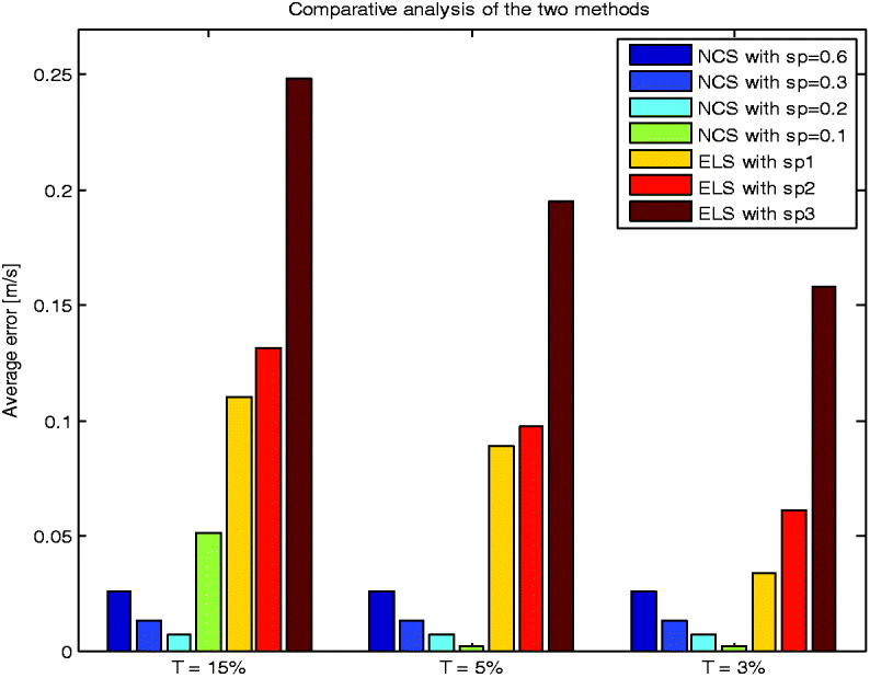
Figure 11. Comparison of the average errors obtained using the NCS and ELS methods.
5. CONCLUSIONS
Unlike the C/A codes, terrain codes are not deterministic sequences. As a result, their correlators do not have a predefined shape, but may be skewed and asymmetric. When applying the early-late scheme, the solution has an error bias caused by the asymmetry of the function. Multipath propagation has the same effect on the GPS signal. Given this fact, two multipath mitigation strategies were adapted to the proposed TRN signal. Their performance, in terms of reducing the bias, was analysed through simulations.
One of the conclusions was that both methods are influenced by the results of the intermediate phase, but in different ways. The NCS method needs more processing time when the remaining bias is higher (T large), but promises the same accuracy. The ELS technique is fast, but its accuracy degrades as T grows. Although ELS (with Sp1) may give more precise solutions on some samples, on average the NCS has the best performance. This conclusion was expected, as the correction introduced by ELS depends on the distance from the peak. The ELS tends to be more useful as a refinement method. However, this leaves space for new ideas. If the intended application needs to be highly accurate ELS can be applied in combination with NCS.
ACKNOWLEDGEMENTS
We would like to thank Erik Theunissen (TU Delft) for helpful suggestions and discussions.


