1 Introduction
Strong, collimated, distinct, continuous flows of plasmas known as astrophysical jets have been observed in various astrophysical contexts over the past century and it is now generally believed that astrophysical jets are driven by magnetohydrodynamic (MHD) forces (Pudritz, Hardcastle & Gabuzda Reference Pudritz, Hardcastle and Gabuzda2012). As noted by Livio (Reference Livio, McEnery, Racusin and Gehrels2011), these jets exist over an enormous range of parameters and are phenomenologically associated with accretion disks. Astrophysical jets can be non-relativistic or relativistic. Jets having dynamics and morphology analogous to non-relativistic astrophysical jets can be created in laboratory experiments and these experiments provide useful insight regarding actual astrophysical jets. The claim that a laboratory experiment has any relevance at all to astrophysical jets might at first sight seem unlikely because the characteristic length and time scales of laboratory experiments are approximately twenty orders of magnitude smaller than those of actual astrophysical jets. However, because the MHD equations have no intrinsic scale, these equations describe both laboratory and astrophysical jets and, as shown by Ryutov, Drake & Remington (Reference Ryutov, Drake and Remington2000) and by Ryutov et al. (Reference Ryutov, Remington, Robey and Drake2001), laboratory experiments can be readily scaled to astrophysical situations to the extent that both are described by MHD.
There are several motivations for studying laboratory experiments that can be scaled to astrophysical jets. First and foremost, the laboratory experiments provide an important test of the validity of the MHD description of astrophysical jets. Second, the laboratory experiments can reveal phenomena such as kinking and Rayleigh–Taylor instability that may occur in actual astrophysical jets. Third, the laboratory experiments can be used to test the validity of MHD codes used to describe actual astrophysical jets and reveal shortcomings or errors in these codes. Fourth, the laboratory experiments can show the transitions to certain types of non-MHD behaviour. Fifth, parameters can be varied in laboratory plasmas to test the predictions of theoretical models. Sixth, the time scale of laboratory experiments is short so that dynamics can be easily followed whereas following the dynamics of actual astrophysical jets can take years, decades or even longer. Finally, the laboratory experiments can in principle be fully diagnosed so that complete understanding might be obtained whereas the diagnostics of actual astrophysical jets are limited so many essential quantities such as the internal magnetic field structure and density profile are poorly known. Laboratory experiments are relatively inexpensive compared to advanced telescopes and spacecraft so a great deal of relevant information and understanding of underlying physics can be obtained with modest resources.
An important feature of experiments is the element of discovery as distinct from the validation of previously existing models. When the experiments started, it was not realized what they would reveal but, as will be shown in this paper, the laboratory experiments have provided unanticipated new insights into the launching, collimation and stability of non-relativistic astrophysical jets and have motivated new models. These show that the jet is comprised of a launching region, a main column and a tip and that different physics dominates in these three regions so the problem is heterogeneous rather than homogeneous. The observations of jet stability have shown existence of primary, secondary and possibly tertiary types of instability where each type drives the next and these observations have shown certain types of coupling between MHD and non-MHD regimes.
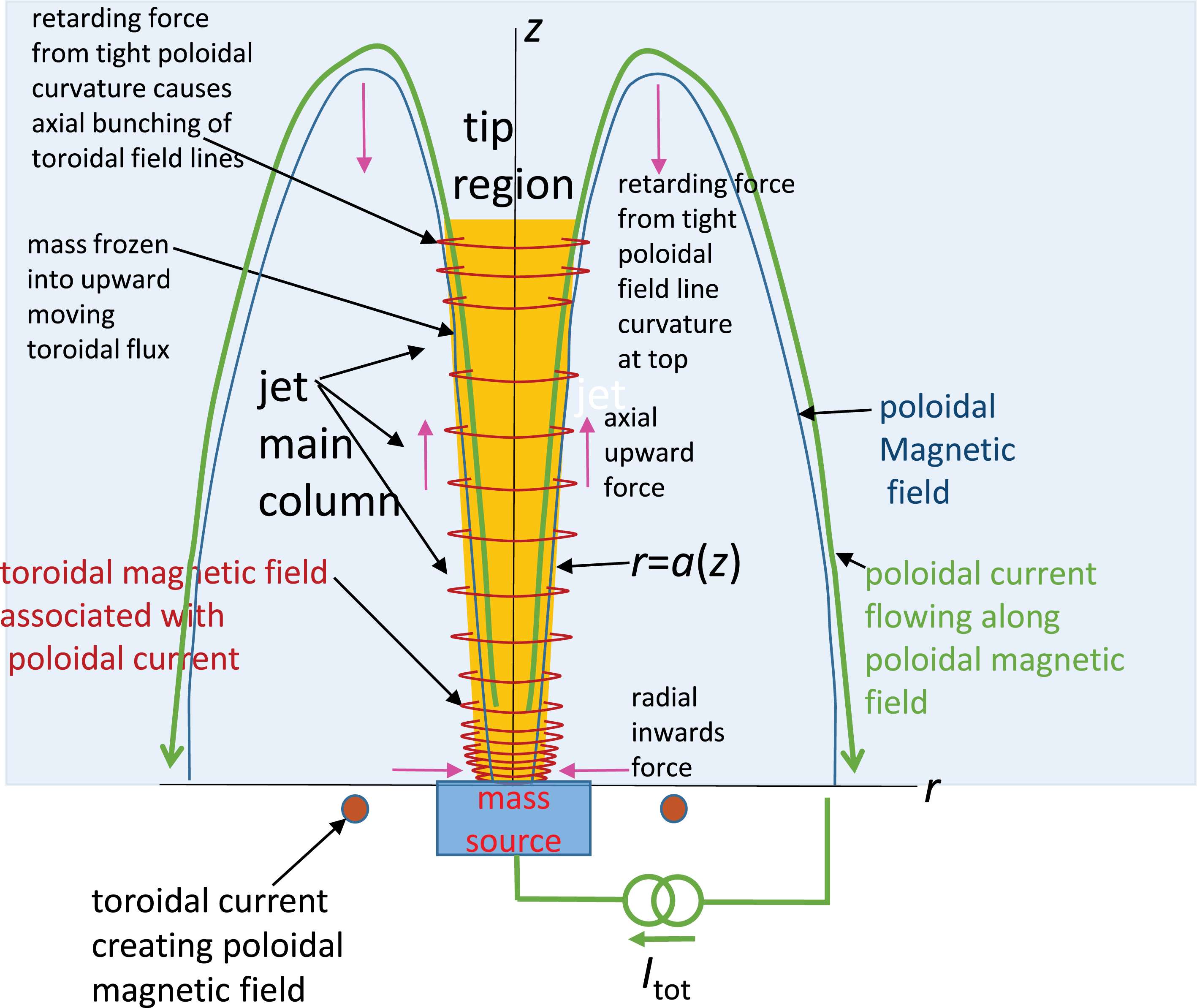
Figure 1. Sketch showing composition of an MHD-driven plasma jet. The jet has a poloidal magnetic field (blue line), a toroidal magnetic field (red circles), plasma (orange), a mass source (blue box) and a current source driving poloidal current (green line). The jet is divided into a main column which is long, slightly flaring and so nearly straight, and a tip region where the poloidal magnetic field has strong curvature.
Because of the huge difference in scale between laboratory experiments and astrophysical jets, laboratory experiments themselves can have very different scales and very different technologies. Three different approaches with three different associated scales and technologies have been used to create laboratory versions of astrophysical jets. These approaches originated from technologies developed for other purposes, namely spheromaks,
 $Z$
-pinches and laser fusion. The spheromak-based approach has been used at Caltech (Hsu & Bellan Reference Hsu and Bellan2002) and has a nominal length scale of 10 cm and a nominal time scale of
$Z$
-pinches and laser fusion. The spheromak-based approach has been used at Caltech (Hsu & Bellan Reference Hsu and Bellan2002) and has a nominal length scale of 10 cm and a nominal time scale of
 $5~\unicode[STIX]{x03BC}\text{s}$
; the
$5~\unicode[STIX]{x03BC}\text{s}$
; the
 $Z$
-pinch approach has been used at Imperial College (Lebedev et al.
Reference Lebedev, Ciardi, Ampleford, Bland, Bott, Chittenden, Hall, Rapley, Jennings and Sherlock2005) and has a nominal length scale of 0.5 cm and a nominal time scale of
$Z$
-pinch approach has been used at Imperial College (Lebedev et al.
Reference Lebedev, Ciardi, Ampleford, Bland, Bott, Chittenden, Hall, Rapley, Jennings and Sherlock2005) and has a nominal length scale of 0.5 cm and a nominal time scale of
 $0.1~\unicode[STIX]{x03BC}\text{s}$
; the laser approach at the Laboratoire d’Utilisation des Lasers Intenses (LULI) (Abertazzi et al.
Reference Abertazzi, Ciardi, Nakatsutsumi, Vinci, Beard, Bonito, Billette, Borghesi, Burkley and Chen2014) has a nominal length scale of 0.2 cm and a nominal time scale of
$0.1~\unicode[STIX]{x03BC}\text{s}$
; the laser approach at the Laboratoire d’Utilisation des Lasers Intenses (LULI) (Abertazzi et al.
Reference Abertazzi, Ciardi, Nakatsutsumi, Vinci, Beard, Bonito, Billette, Borghesi, Burkley and Chen2014) has a nominal length scale of 0.2 cm and a nominal time scale of
 $0.01~\unicode[STIX]{x03BC}\text{s}$
; the laser approach at the University of Rochester (Li et al.
Reference Li, Tzeferacos, Lamb, Gregori, Norreys, Rosenberg, Follett, Froula, Koenig and Seguin2016) has a nominal length scale of 0.5 cm and a nominal time scale of
$0.01~\unicode[STIX]{x03BC}\text{s}$
; the laser approach at the University of Rochester (Li et al.
Reference Li, Tzeferacos, Lamb, Gregori, Norreys, Rosenberg, Follett, Froula, Koenig and Seguin2016) has a nominal length scale of 0.5 cm and a nominal time scale of
 $0.001~\unicode[STIX]{x03BC}\text{s}$
. There is thus a two to three order of magnitude difference between the parameters of these experiments, but this difference pales in comparison to the approximately twenty orders of magnitude difference they all have relative to actual astrophysical jets. Besides differing in time and length scales, the three different approaches differ in how magnetic fields are generated, the magnitude of the magnetic field, whether the magnetic fields are poloidal, toroidal or both, the type of diagnostics used, how often the experiment can be operated and the plasma density and temperature. The Caltech experiment has both toroidal and poloidal magnetic fields, can be internally probed, has a well-defined changing morphology and the plasma can be created non-destructively once every two minutes so it is possible to have large numbers of plasma shots. The
$0.001~\unicode[STIX]{x03BC}\text{s}$
. There is thus a two to three order of magnitude difference between the parameters of these experiments, but this difference pales in comparison to the approximately twenty orders of magnitude difference they all have relative to actual astrophysical jets. Besides differing in time and length scales, the three different approaches differ in how magnetic fields are generated, the magnitude of the magnetic field, whether the magnetic fields are poloidal, toroidal or both, the type of diagnostics used, how often the experiment can be operated and the plasma density and temperature. The Caltech experiment has both toroidal and poloidal magnetic fields, can be internally probed, has a well-defined changing morphology and the plasma can be created non-destructively once every two minutes so it is possible to have large numbers of plasma shots. The
 $Z$
-pinch approach at Imperial College has a toroidal magnetic field but no poloidal field and has X-ray imaging rather than probes. The University of Rochester laser experiment has a self-generated magnetic field which is assumed to contain poloidal and toroidal components. The LULI laser experiment has an externally imposed poloidal magnetic field. The last stage of the apparatus is destroyed on each shot of the
$Z$
-pinch approach at Imperial College has a toroidal magnetic field but no poloidal field and has X-ray imaging rather than probes. The University of Rochester laser experiment has a self-generated magnetic field which is assumed to contain poloidal and toroidal components. The LULI laser experiment has an externally imposed poloidal magnetic field. The last stage of the apparatus is destroyed on each shot of the
 $Z$
-pinch experiment and on both types of laser experiments so the number of shots is limited to at most a few per day.
$Z$
-pinch experiment and on both types of laser experiments so the number of shots is limited to at most a few per day.
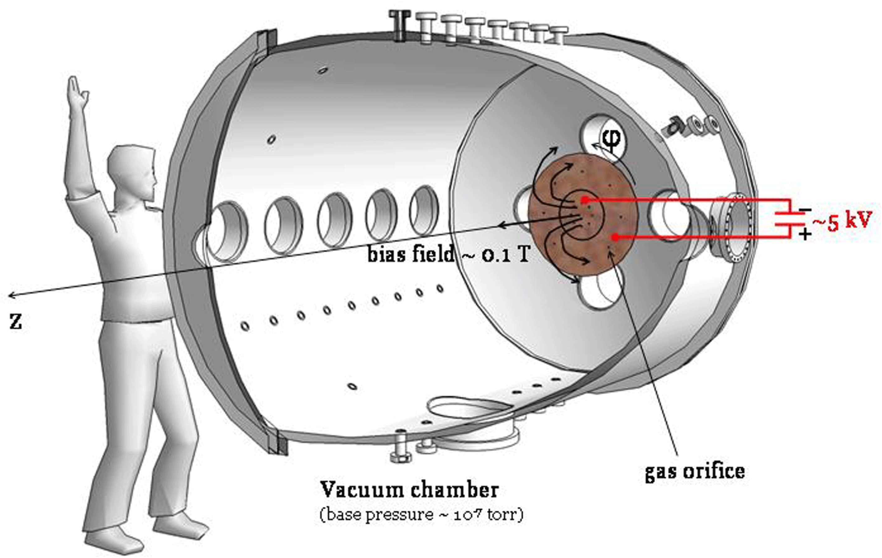
Figure 2. Sketch of experimental layout showing disk and annulus electrodes, poloidal magnetic field produced by coil behind gap between disk and and annulus and schematic of the power supply that provides high voltage for breakdown and then drives the jet current. The eight gas holes on each of the disk and annulus are shown as black dots.
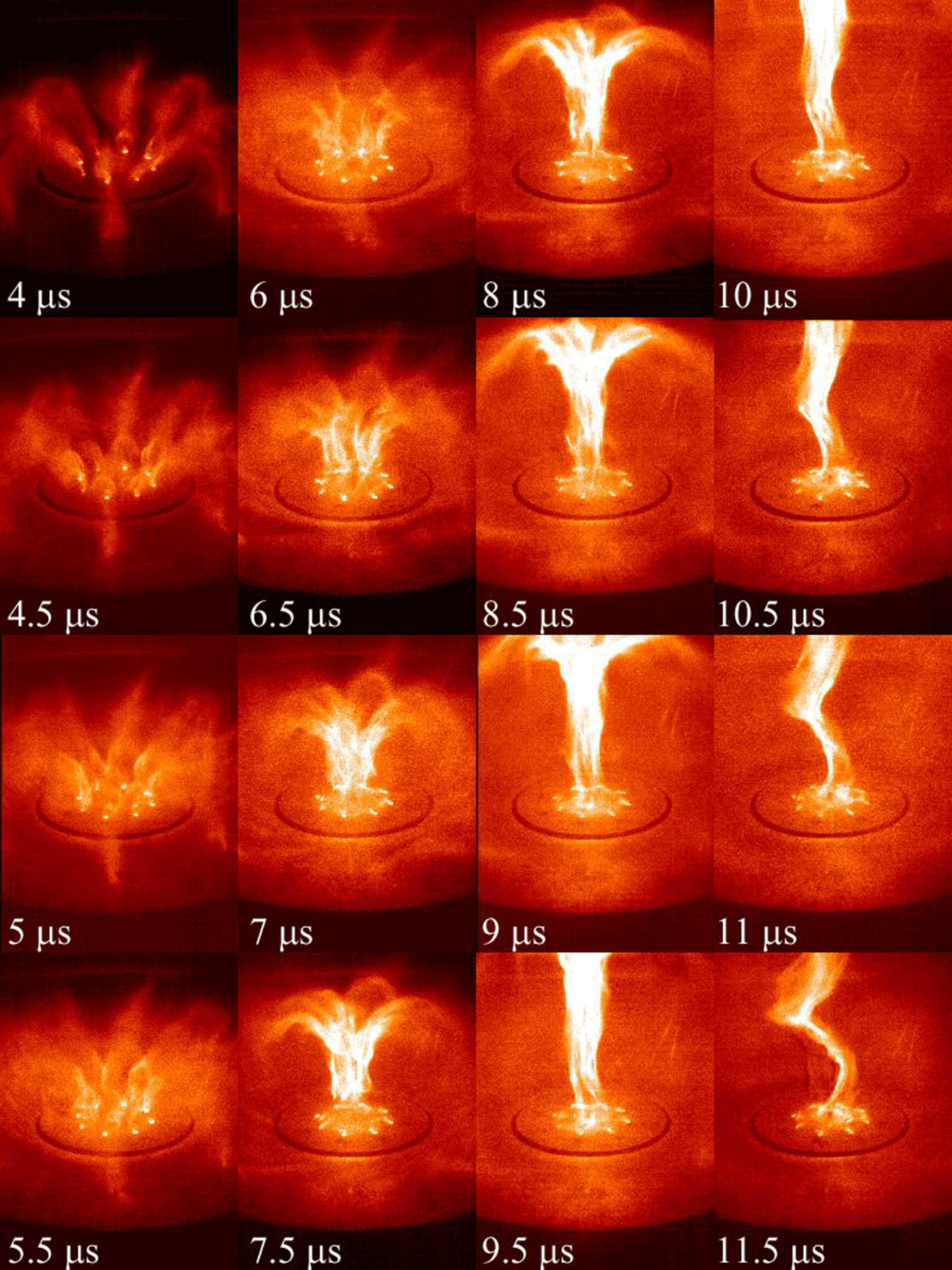
Figure 3. Typical jet formation and propagation in Caltech experiment. [Reprinted figure with permission from You, Yun and Bellan, Physical Review Letters 95, 045002 (2005). Copyright 2005 by the American Physical Society.]
This paper will focus on the Caltech experiment but the concepts to be described are also relevant to the other experiments and to actual astrophysical jets. The generic layout of the Caltech laboratory jet and presumably of an astrophysical jet is shown in figure 1. The Caltech experiment takes place in a 1.4 m diameter, 2 m long vacuum chamber sketched in figure 2. The jet in figure 2 emanates from the concentric set of electrodes located at the far right end of the chamber. The electrodes consist of a 20 cm diameter copper disk surrounded by a coplanar 50 cm diameter copper annulus with a 6 mm gap between the disk and the annulus so that the disk and annulus can be at different electrostatic potentials. A coil coaxial with the disk and annulus and located just behind the gap generates a dipole-like magnetic field that links the disk to the annulus; this magnetic field corresponds to the blue line labelled ‘poloidal magnetic field’ in figure 1. Figure 3 from You, Yun & Bellan (Reference You, Yun and Bellan2005) shows the typical formation, propagation and kink destabilization of a jet formed in this experiment (note that vertically upward motion in figure 3 corresponds to right-to-left motion in figure 2).
Section 2 presents a theoretical model of this jet using two complementary descriptions of the magnetic force, where the first emphasizes the importance of scalar flux functions and the second emphasizes the importance of magnetic field line curvature and gradients of field strength. Section 3 describes in detail the set-up of the experiment sketched in figure 2 that creates laboratory-scale MHD-driven jets. Section 4 describes measurements of the velocity of these jets. Section 5 describes the kink instability of these jets. Section 6 describes how kinking can establish conditions for a Rayleigh–Taylor instability. Section 7 describes several consequences of the Rayleigh–Taylor instability. Section 8 summarizes the results of a numerical simulation of the jet experiment. Section 9 describes an experiment where a jet collides with a target cloud, slows down and becomes compressed. Section 10 discusses how the laboratory set-up for launching an MHD jet needs to be replaced by an equivalently effective launching scheme for an actual astrophysical jet. Section 11 provides a brief summary. Appendix A provides a brief discussion of the experiments at Imperial College, the University of Rochester and at LULI with certain differences from and similarities to the Caltech experiment identified.
2 Theory
2.1 Flux functions
The discussion will be confined to non-relativistic jets that are governed by ideal MHD and that involve combined poloidal and toroidal magnetic fields. These jets involve the full set of ideal MHD equations, namely the equation of motion, induction equation, continuity equation,
 $$\begin{eqnarray}\displaystyle & \displaystyle \unicode[STIX]{x1D70C}\frac{\text{d}\boldsymbol{U}}{\text{d}t}=\boldsymbol{J}\times \boldsymbol{B}-\unicode[STIX]{x1D735}P & \displaystyle\end{eqnarray}$$
 $$\begin{eqnarray}\displaystyle & \displaystyle \frac{\unicode[STIX]{x2202}\boldsymbol{B}}{\unicode[STIX]{x2202}t}=\unicode[STIX]{x1D735}\times (\boldsymbol{U}\times \boldsymbol{B}) & \displaystyle\end{eqnarray}$$
 $$\begin{eqnarray}\displaystyle & \displaystyle \frac{\unicode[STIX]{x2202}\unicode[STIX]{x1D70C}}{\unicode[STIX]{x2202}t}+\unicode[STIX]{x1D735}\boldsymbol{\cdot }(\unicode[STIX]{x1D70C}\boldsymbol{U})=0 & \displaystyle\end{eqnarray}$$
and an equation of state that, depending on the physical circumstances, can be adiabatic, isothermal or the result of a more detailed energy equation. Since (2.1)–(2.3) have no intrinsic scale, they can be expressed in a dimensionless form and it is this property that allows laboratory plasma experiments to be scaled to solar or astrophysical regimes.
2.2 Scaling of laboratory experiments to astrophysical situations
The method for scaling was developed by Ryutov et al. (Reference Ryutov, Drake and Remington2000, Reference Ryutov, Remington, Robey and Drake2001) and will now be briefly summarized. A given situation (e.g. laboratory experiment or actual astrophysical jet) is characterized by a reference mass density
 $\unicode[STIX]{x1D70C}_{0}$
, a reference magnetic field
$\unicode[STIX]{x1D70C}_{0}$
, a reference magnetic field
 $B_{0}$
, a reference length
$B_{0}$
, a reference length
 $L$
and a reference pressure
$L$
and a reference pressure
 $P_{0}$
so that all lengths, mass densities, magnetic fields and pressures are normalized to these reference quantities. These reference quantities provide convenient units by which parameters can be measured so when measured in terms of these reference quantities all parameters are of order unity. The first two reference quantities define a reference Alfvén velocity
$P_{0}$
so that all lengths, mass densities, magnetic fields and pressures are normalized to these reference quantities. These reference quantities provide convenient units by which parameters can be measured so when measured in terms of these reference quantities all parameters are of order unity. The first two reference quantities define a reference Alfvén velocity
 $v_{A0}=B_{0}/\sqrt{\unicode[STIX]{x1D707}_{0}\unicode[STIX]{x1D70C}_{0}}$
which upon combination with the third reference quantity defines a reference time
$v_{A0}=B_{0}/\sqrt{\unicode[STIX]{x1D707}_{0}\unicode[STIX]{x1D70C}_{0}}$
which upon combination with the third reference quantity defines a reference time
 $\unicode[STIX]{x1D70F}=L/v_{A0}$
. The last two reference quantities define a reference
$\unicode[STIX]{x1D70F}=L/v_{A0}$
. The last two reference quantities define a reference
 $\unicode[STIX]{x1D6FD}=\unicode[STIX]{x1D707}_{0}P_{0}/B_{0}^{2}$
. Using Ampere’s law (2.1) can be expressed as
$\unicode[STIX]{x1D6FD}=\unicode[STIX]{x1D707}_{0}P_{0}/B_{0}^{2}$
. Using Ampere’s law (2.1) can be expressed as
 $$\begin{eqnarray}\unicode[STIX]{x1D70C}\left(\frac{\unicode[STIX]{x2202}\boldsymbol{U}}{\unicode[STIX]{x2202}t}+\boldsymbol{U}\boldsymbol{\cdot }\unicode[STIX]{x1D735}\boldsymbol{U}\right)=\frac{(\unicode[STIX]{x1D735}\times \boldsymbol{B})}{\unicode[STIX]{x1D707}_{0}}\times \boldsymbol{B}-\unicode[STIX]{x1D735}P.\end{eqnarray}$$
By defining the normalized dimensionless quantities
 $\bar{t}=t/\unicode[STIX]{x1D70F},\bar{\unicode[STIX]{x1D70C}}=\unicode[STIX]{x1D70C}/\unicode[STIX]{x1D70C}_{0},\bar{\unicode[STIX]{x1D735}}=L\unicode[STIX]{x1D735}$
,
$\bar{t}=t/\unicode[STIX]{x1D70F},\bar{\unicode[STIX]{x1D70C}}=\unicode[STIX]{x1D70C}/\unicode[STIX]{x1D70C}_{0},\bar{\unicode[STIX]{x1D735}}=L\unicode[STIX]{x1D735}$
,
 $\bar{\boldsymbol{B}}=\boldsymbol{B}/B_{0}$
,
$\bar{\boldsymbol{B}}=\boldsymbol{B}/B_{0}$
,
 $\bar{\boldsymbol{U}}=\boldsymbol{U}/v_{A0}$
, equations (2.2), (2.3) and (2.4) can be expressed as
$\bar{\boldsymbol{U}}=\boldsymbol{U}/v_{A0}$
, equations (2.2), (2.3) and (2.4) can be expressed as
 $$\begin{eqnarray}\displaystyle & \displaystyle \bar{\unicode[STIX]{x1D70C}}\left(\frac{\unicode[STIX]{x2202}\bar{\boldsymbol{U}}}{\unicode[STIX]{x2202}\bar{t}}+\bar{\boldsymbol{U}}\boldsymbol{\cdot }\bar{\unicode[STIX]{x1D735}}\bar{\boldsymbol{U}}\right)=(\bar{\unicode[STIX]{x1D735}}\times \bar{\boldsymbol{B}})\times \bar{\boldsymbol{B}}-\unicode[STIX]{x1D6FD}\bar{\unicode[STIX]{x1D735}}\bar{P} & \displaystyle\end{eqnarray}$$
 $$\begin{eqnarray}\displaystyle & \displaystyle \frac{\unicode[STIX]{x2202}\bar{\boldsymbol{B}}}{\unicode[STIX]{x2202}\bar{t}}=\bar{\unicode[STIX]{x1D735}}\times (\bar{\boldsymbol{U}}\times \bar{\boldsymbol{B}}) & \displaystyle\end{eqnarray}$$
 $$\begin{eqnarray}\displaystyle & \displaystyle \frac{\unicode[STIX]{x2202}\bar{\unicode[STIX]{x1D70C}}}{\unicode[STIX]{x2202}\bar{t}}+\bar{\unicode[STIX]{x1D735}}\boldsymbol{\cdot }(\bar{\unicode[STIX]{x1D70C}}\bar{\boldsymbol{U}})=0. & \displaystyle\end{eqnarray}$$
If a laboratory and an astrophysical plasma have the same
 $\unicode[STIX]{x1D6FD}$
then (2.5)–(2.7) will be identical for the two plasmas and so, if the normalized boundary and initial conditions are the same for the laboratory and astrophysical plasmas, then the two plasmas will evolve in identical ways. On denoting the laboratory plasma by ‘
$\unicode[STIX]{x1D6FD}$
then (2.5)–(2.7) will be identical for the two plasmas and so, if the normalized boundary and initial conditions are the same for the laboratory and astrophysical plasmas, then the two plasmas will evolve in identical ways. On denoting the laboratory plasma by ‘
 $s$
’ for small and the astrophysical plasma by ‘
$s$
’ for small and the astrophysical plasma by ‘
 $l$
’ for large, the scaling between the two plasmas is determined from three parameters:
$l$
’ for large, the scaling between the two plasmas is determined from three parameters:
 $$\begin{eqnarray}c_{1}=\frac{L_{s}}{L_{l}},\quad c_{2}=\frac{\unicode[STIX]{x1D70C}_{0s}}{\unicode[STIX]{x1D70C}_{0l}},\quad c_{3}=\frac{P_{0s}}{P_{0l}}.\end{eqnarray}$$
Since the two plasmas have the same
 $\unicode[STIX]{x1D6FD}$
, it is seen that
$\unicode[STIX]{x1D6FD}$
, it is seen that
 $$\begin{eqnarray}\unicode[STIX]{x1D6FD}=\frac{\unicode[STIX]{x1D707}_{0}P_{0s}}{B_{0s}^{2}}=\frac{\unicode[STIX]{x1D707}_{0}P_{0l}}{B_{0l}^{2}}\end{eqnarray}$$
so
 $$\begin{eqnarray}B_{0s}=B_{0l}\sqrt{\frac{P_{0s}}{P_{0l}}}=\sqrt{c_{3}}B_{0l}.\end{eqnarray}$$
The reference Alfvén velocity of the laboratory plasma is
 $$\begin{eqnarray}v_{A0s}=\frac{B_{0s}}{\sqrt{\unicode[STIX]{x1D707}_{0}\unicode[STIX]{x1D70C}_{0s}}}=\frac{\sqrt{c_{3}}B_{0l}}{\sqrt{\unicode[STIX]{x1D707}_{0}c_{2}\unicode[STIX]{x1D70C}_{0l}}}=\sqrt{\frac{c_{3}}{c_{2}}}v_{A0l}\end{eqnarray}$$
and the reference time of the laboratory plasma is
 $$\begin{eqnarray}\unicode[STIX]{x1D70F}_{s}=\frac{L_{s}}{v_{A0s}}=\frac{c_{1}L_{l}}{\sqrt{\displaystyle \frac{c_{3}}{c_{2}}}v_{A0l}}=c_{1}\sqrt{\frac{c_{2}}{c_{3}}}\unicode[STIX]{x1D70F}_{l}.\end{eqnarray}$$
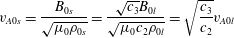
As an example of how this scaling can be implemented, suppose that a laboratory plasma composed of hydrogen has a reference time
 $\unicode[STIX]{x1D70F}_{s}=1~\unicode[STIX]{x03BC}\text{s}$
(this does not mean that the laboratory plasma lasts one
$\unicode[STIX]{x1D70F}_{s}=1~\unicode[STIX]{x03BC}\text{s}$
(this does not mean that the laboratory plasma lasts one
 $1~\unicode[STIX]{x03BC}\text{s}$
but rather that this is the convenient unit by which time is measured), a reference length
$1~\unicode[STIX]{x03BC}\text{s}$
but rather that this is the convenient unit by which time is measured), a reference length
 $L_{s}=10~\text{cm}$
, a reference density
$L_{s}=10~\text{cm}$
, a reference density
 $n_{s}=10^{16}~\text{cm}^{-3}$
and a reference temperature 2 eV. Suppose that a hydrogen astrophysical jet has a reference density
$n_{s}=10^{16}~\text{cm}^{-3}$
and a reference temperature 2 eV. Suppose that a hydrogen astrophysical jet has a reference density
 $n_{l}=2\times 10^{3}~\text{cm}^{-3}$
, a reference temperature 10 eV and a reference length 100 a.u., i.e.
$n_{l}=2\times 10^{3}~\text{cm}^{-3}$
, a reference temperature 10 eV and a reference length 100 a.u., i.e.
 $L_{l}=1.5\times 10^{13}~\text{m}$
. Using these relations it is seen that
$L_{l}=1.5\times 10^{13}~\text{m}$
. Using these relations it is seen that
 $c_{1}=6.7\times 10^{-15}$
,
$c_{1}=6.7\times 10^{-15}$
,
 $c_{2}=5\times 10^{12}$
and
$c_{2}=5\times 10^{12}$
and
 $c_{3}=10^{12}$
. Using (2.10), a 1 kG magnetic field in the laboratory experiment would scale to a 1 mG magnetic field in the astrophysical jet, a velocity of
$c_{3}=10^{12}$
. Using (2.10), a 1 kG magnetic field in the laboratory experiment would scale to a 1 mG magnetic field in the astrophysical jet, a velocity of
 $50~\text{km}~\text{s}^{-1}$
in the laboratory experiment would scale to a velocity
$50~\text{km}~\text{s}^{-1}$
in the laboratory experiment would scale to a velocity
 $112~\text{km}~\text{s}^{-1}$
in the astrophysical jet and a time of
$112~\text{km}~\text{s}^{-1}$
in the astrophysical jet and a time of
 $10~\unicode[STIX]{x03BC}\text{s}$
in the laboratory experiment would scale to a time of 21 years for the astrophysical jet. The reference quantities chosen for the laboratory experiment are nominal values observed in the Caltech laboratory experiment and the scaled astrophysical jet time, length, velocity, density, magnetic field and temperature are consistent in order of magnitude with values reported in Wassell et al. (Reference Wassell, Grady, Woodgate, Kimble and Bruhweiler2006). Thus, to the extent that both the laboratory and astrophysical jet plasmas are described by (2.5)–(2.7), they will have the same behaviour when described in normalized quantities and the scaling of laboratory and astrophysical quantities will be given by (2.8)–(2.12). A similar scaling has been provided by Li et al. (Reference Li, Tzeferacos, Lamb, Gregori, Norreys, Rosenberg, Follett, Froula, Koenig and Seguin2016) to show that the parameters of the University of Rochester laser-driven jet experiment scale to the Crab Nebula.
$10~\unicode[STIX]{x03BC}\text{s}$
in the laboratory experiment would scale to a time of 21 years for the astrophysical jet. The reference quantities chosen for the laboratory experiment are nominal values observed in the Caltech laboratory experiment and the scaled astrophysical jet time, length, velocity, density, magnetic field and temperature are consistent in order of magnitude with values reported in Wassell et al. (Reference Wassell, Grady, Woodgate, Kimble and Bruhweiler2006). Thus, to the extent that both the laboratory and astrophysical jet plasmas are described by (2.5)–(2.7), they will have the same behaviour when described in normalized quantities and the scaling of laboratory and astrophysical quantities will be given by (2.8)–(2.12). A similar scaling has been provided by Li et al. (Reference Li, Tzeferacos, Lamb, Gregori, Norreys, Rosenberg, Follett, Froula, Koenig and Seguin2016) to show that the parameters of the University of Rochester laser-driven jet experiment scale to the Crab Nebula.
2.3 Validity of scaling and of ideal MHD assumption
This scaling argument fails if (2.5)–(2.7) become invalid descriptions. This failure will happen when terms that have been dropped to obtain these equations become important. Situations where the equations become invalid descriptions include:
(i) The velocity approaches the speed of light. This is not an issue for laboratory plasmas or for jets associated with protoplanetary disks as these jets have velocities that are much less than 1 % of the speed of light.
(ii) The Lundquist number
 $S=\unicode[STIX]{x1D707}_{0}v_{A0}L/\unicode[STIX]{x1D702}$
becomes so small as to be of order unity; here
$\unicode[STIX]{x1D702}$
is the electrical resistivity.
$S$
is of the order of
$10^{2}$
for the laboratory plasma and since the laboratory and astrophysical plasmas have similar velocities and temperatures the main difference in the terms contributing to
$S$
is the length
$L$
so the astrophysical jet has
$S\sim 10^{17}$
. Since the term depending on
$S$
that was dropped from (2.6) scales as
$1/S$
, this term can certainly be omitted as all other terms have been defined by choice of reference parameters to be of order unity.
$S=\unicode[STIX]{x1D707}_{0}v_{A0}L/\unicode[STIX]{x1D702}$
becomes so small as to be of order unity; here
$\unicode[STIX]{x1D702}$
is the electrical resistivity.
$S$
is of the order of
$10^{2}$
for the laboratory plasma and since the laboratory and astrophysical plasmas have similar velocities and temperatures the main difference in the terms contributing to
$S$
is the length
$L$
so the astrophysical jet has
$S\sim 10^{17}$
. Since the term depending on
$S$
that was dropped from (2.6) scales as
$1/S$
, this term can certainly be omitted as all other terms have been defined by choice of reference parameters to be of order unity.(iii) The Hall term in the generalized Ohm’s law becomes important. This happens when spatial gradients of the magnetic field have length scales that are smaller than the ion skin depth
$d_{i}=c/\unicode[STIX]{x1D714}_{pi}$
. As will be discussed in § 7 the laboratory plasma marginally satisfies the condition
$L\gg d_{i}$
but can transiently access regimes where
$L<d_{i}$
in which case Hall terms become important. It is possible that this also happens in certain astrophysical jets but
$d_{i}$
is many orders of magnitude too small to be resolved by observations using foreseeable technology.(iv)
$J/ne$
becomes large enough to become comparable to the thermal velocity or the phase velocity of some plasma wave (e.g. acoustic, Alfvén) in which case kinetic effects become important. The laboratory plasma generally has suitably small
$J/ne$
to avoid this but situations can develop where the condition is violated. This could also happen in certain astrophysical situations if sufficiently strong localized magnetic field gradients developed. Extremely large
$J/ne$
would likely result in production of energetic particles; this situation is outside the scope of MHD. Large
$J/ne$
could destabilize kinetic modes in some situations and in other situations would result in runaway electrons if
$\unicode[STIX]{x1D702}J$
exceeds the Dreicer electric field (Dreicer Reference Dreicer1959; Bellan Reference Bellan2006). The small
$J/ne$
assumption is marginally satisfied in laboratory plasmas but can be violated in certain situations.(v) Resistive effects become dominant. Ideal MHD means that Ohm’s law can be written as
$\boldsymbol{E}+\boldsymbol{U}\times \boldsymbol{B}=0$
rather than as
$\boldsymbol{E}+\boldsymbol{U}\times \boldsymbol{B}=\unicode[STIX]{x1D702}\boldsymbol{J}$
. Taking the curl of the latter equation gives (2.13)so dropping the resistive term corresponds to assuming that$$\begin{eqnarray}-\frac{\unicode[STIX]{x2202}\boldsymbol{B}}{\unicode[STIX]{x2202}t}+\unicode[STIX]{x1D735}\times (\boldsymbol{U}\times \boldsymbol{B})=\frac{\unicode[STIX]{x1D702}}{\unicode[STIX]{x1D707}_{0}}\unicode[STIX]{x1D735}\times \unicode[STIX]{x1D735}\times \boldsymbol{B}\end{eqnarray}$$
$\unicode[STIX]{x1D702}\unicode[STIX]{x1D70F}/\unicode[STIX]{x1D707}_{0}\ll L^{2}$
which means that the characteristic time
$\unicode[STIX]{x1D70F}$
is much shorter than the time for magnetic field to diffuse across the plasma. Because of the large scale lengths in astrophysical problems this is easily satisfied. This constrains the duration of the laboratory experiment to be short compared to the resistive diffusion time
$\unicode[STIX]{x1D707}_{0}L^{2}/\unicode[STIX]{x1D702}$
; thus, since
$\unicode[STIX]{x1D702}$
scales as
$T^{-3/2}$
the laboratory experiment should not be too cold. Discarding the resistive term in (2.13) does not preclude the collision mean free path from being smaller than the system size and so ideal MHD does not require the plasma to be collisionless, only that events take place much faster than the resistive diffusion time.(vi) The plasma is so collisionless that the pressure is no longer isotropic. Ideal MHD assumes there are sufficient collisions for the plasma pressure to be represented by an isotropic scalar. As the collisionality is progressively reduced, plasma regimes change in a sequence as follows: pressure becomes anisotropic so a double adiabatic description is required (Chew, Goldberger & Low Reference Chew, Goldberger and Low1956), the ion and electron temperatures become disconnected from each other and finally the velocity distribution function becomes completely non-Maxwellian so the concept of temperature ceases to exist.


In summary, the laboratory plasma generally satisfies the assumptions required for ideal MHD (enough collisions to make the pressure isotropic but not so many that resistive diffusion causes unfreezing of the magnetic flux from the plasma, the Hall term can be dropped, kinetic effects are unimportant). However, laboratory plasmas can also access regimes where these assumptions are violated and so laboratory plasmas can reveal information about the coupling between MHD and non-MHD phenomena.
2.4 Relation to Taylor state and spheromaks
The reversed field pinch (RFP) is a toroidal magnetic device intended to confine a plasma relevant to controlled thermonuclear fusion studies (Bodin Reference Bodin1990). RFP plasmas had been routinely observed during the 1960s and early 1970s to spontaneously self-organize into a simple well-defined state that could be modelled using Bessel functions together with the assumption of zero hydrodynamic pressure. However, it was not understood why this self-organization happened. Taylor (Reference Taylor1974) argued that self-organization takes place because instabilities cause a zero-pressure plasma to seek a minimum-energy MHD equilibrium (i.e. a minimum of
 $\int B^{2}\,\text{d}^{3}r$
) while simultaneously conserving magnetic helicity (i.e.
$\int B^{2}\,\text{d}^{3}r$
) while simultaneously conserving magnetic helicity (i.e.
 $\int \boldsymbol{A}\boldsymbol{\cdot }\boldsymbol{B}\,\text{d}^{3}r$
). The quantity
$\int \boldsymbol{A}\boldsymbol{\cdot }\boldsymbol{B}\,\text{d}^{3}r$
). The quantity
 $\boldsymbol{A}$
is the vector potential and magnetic helicity is a measure of flux linkages with each other and also is related to twist. A similar argument had been provided earlier by Woltjer (Reference Woltjer1958) for astrophysical contexts. The basis for the Woltjer–Taylor argument is that a scale separation exists between the rates of dissipation of energy and of magnetic helicity and if this scale separation is extreme, there is substantial energy dissipation but negligible helicity dissipation. Although the energy dissipation is substantial, the energy cannot decay to zero because energy depends on
$\boldsymbol{A}$
is the vector potential and magnetic helicity is a measure of flux linkages with each other and also is related to twist. A similar argument had been provided earlier by Woltjer (Reference Woltjer1958) for astrophysical contexts. The basis for the Woltjer–Taylor argument is that a scale separation exists between the rates of dissipation of energy and of magnetic helicity and if this scale separation is extreme, there is substantial energy dissipation but negligible helicity dissipation. Although the energy dissipation is substantial, the energy cannot decay to zero because energy depends on
 $B^{2}$
so
$B^{2}$
so
 $\boldsymbol{B}$
would have to vanish everywhere which would then cause the helicity to vanish. Thus, the system will seek a minimum-energy state that conserves helicity. Minimizing energy while conserving helicity can be expressed as a variational problem the solution of which is
$\boldsymbol{B}$
would have to vanish everywhere which would then cause the helicity to vanish. Thus, the system will seek a minimum-energy state that conserves helicity. Minimizing energy while conserving helicity can be expressed as a variational problem the solution of which is
 $$\begin{eqnarray}\unicode[STIX]{x1D735}\times \boldsymbol{B}=\unicode[STIX]{x1D706}\boldsymbol{B},\end{eqnarray}$$
where
 $\unicode[STIX]{x1D706}$
is the smallest constant that satisfies imposed boundary conditions. Equation (2.14) implies
$\unicode[STIX]{x1D706}$
is the smallest constant that satisfies imposed boundary conditions. Equation (2.14) implies
 $\boldsymbol{J}\times \boldsymbol{B}=0$
and so is a force-free state. In cylindrical geometry the components of (2.14) are
$\boldsymbol{J}\times \boldsymbol{B}=0$
and so is a force-free state. In cylindrical geometry the components of (2.14) are
 $$\begin{eqnarray}\displaystyle \unicode[STIX]{x1D707}_{0}J_{r} & = & \displaystyle \unicode[STIX]{x1D706}B_{r}\end{eqnarray}$$
 $$\begin{eqnarray}\displaystyle \unicode[STIX]{x1D707}_{0}J_{\unicode[STIX]{x1D719}} & = & \displaystyle \unicode[STIX]{x1D706}B_{\unicode[STIX]{x1D719}}\end{eqnarray}$$
 $$\begin{eqnarray}\displaystyle \unicode[STIX]{x1D707}_{0}J_{z} & = & \displaystyle \unicode[STIX]{x1D706}B_{z};\end{eqnarray}$$
 $\unicode[STIX]{x1D706}$
can be interpreted in several ways: it can be considered an eigenvalue in (2.14), a measure of twist or as an extensive variable conjugate to helicity that is analogous to temperature being an extensive variable conjugate to heat in thermodynamics (Bellan Reference Bellan2000, Reference Bellan2018b
). The analysis leading to (2.14) involves presumption of a flux-conserving boundary which is the property of a perfectly conducting wall. This flux-conserving property enables setting to zero various terms that show up when integrating by parts to establish (2.14). The solutions to this equation are in quite good agreement with a large number of observed plasmas such as RFPs, spheromaks and solar corona loops. Spheromaks are Taylor states confined by a bounding wall that has the topology of a spheroid (Rosenbluth & Bussac Reference Rosenbluth and Bussac1979; Jarboe Reference Jarboe1994; Bellan Reference Bellan2000, Reference Bellan2018b
); this is in contrast to RFPs where the Taylor state is confined by a bounding wall that has the topology of a toroid.
$\unicode[STIX]{x1D706}$
can be interpreted in several ways: it can be considered an eigenvalue in (2.14), a measure of twist or as an extensive variable conjugate to helicity that is analogous to temperature being an extensive variable conjugate to heat in thermodynamics (Bellan Reference Bellan2000, Reference Bellan2018b
). The analysis leading to (2.14) involves presumption of a flux-conserving boundary which is the property of a perfectly conducting wall. This flux-conserving property enables setting to zero various terms that show up when integrating by parts to establish (2.14). The solutions to this equation are in quite good agreement with a large number of observed plasmas such as RFPs, spheromaks and solar corona loops. Spheromaks are Taylor states confined by a bounding wall that has the topology of a spheroid (Rosenbluth & Bussac Reference Rosenbluth and Bussac1979; Jarboe Reference Jarboe1994; Bellan Reference Bellan2000, Reference Bellan2018b
); this is in contrast to RFPs where the Taylor state is confined by a bounding wall that has the topology of a toroid. Integrating (2.14) over an arbitrary surface
 $S$
gives
$S$
gives
 $$\begin{eqnarray}\int _{S}\,\text{d}\boldsymbol{s}\boldsymbol{\cdot }\unicode[STIX]{x1D735}\times \boldsymbol{B}=\unicode[STIX]{x1D706}\int _{S}\,\text{d}\boldsymbol{s}\boldsymbol{\cdot }\boldsymbol{B}\end{eqnarray}$$
or
 $$\begin{eqnarray}\unicode[STIX]{x1D707}_{0}I=\unicode[STIX]{x1D706}\unicode[STIX]{x1D713},\end{eqnarray}$$
where
 $I$
and
$I$
and
 $\unicode[STIX]{x1D713}$
are respectively the electric current and the magnetic flux passing through the surface
$\unicode[STIX]{x1D713}$
are respectively the electric current and the magnetic flux passing through the surface
 $S$
. Equation (2.14) results from assuming a zero-pressure equilibrium that has relaxed to its lowest-energy state while conserving magnetic helicity. One type of system for creating spheromaks, the coaxial helicity injector, has essentially the same topology as that sketched in figure 1 and so the formation process of the spheromak using this system is closely related to astrophysical jets (Bellan Reference Bellan2018b
). To the extent that an astrophysical jet has low
$S$
. Equation (2.14) results from assuming a zero-pressure equilibrium that has relaxed to its lowest-energy state while conserving magnetic helicity. One type of system for creating spheromaks, the coaxial helicity injector, has essentially the same topology as that sketched in figure 1 and so the formation process of the spheromak using this system is closely related to astrophysical jets (Bellan Reference Bellan2018b
). To the extent that an astrophysical jet has low
 $\unicode[STIX]{x1D6FD}$
(i.e.
$\unicode[STIX]{x1D6FD}$
(i.e.
 $P$
small compared to
$P$
small compared to
 $B^{2}/2\unicode[STIX]{x1D707}_{0}$
) and has a twisted magnetic field (i.e. has magnetic helicity), an astrophysical jet is closely related to a spheromak, the difference being that the pressure is not exactly zero, the system is not in equilibrium but instead evolves in time and poloidal magnetic field lines intercept a boundary (
$B^{2}/2\unicode[STIX]{x1D707}_{0}$
) and has a twisted magnetic field (i.e. has magnetic helicity), an astrophysical jet is closely related to a spheromak, the difference being that the pressure is not exactly zero, the system is not in equilibrium but instead evolves in time and poloidal magnetic field lines intercept a boundary (
 $z=0$
plane in figure 1). This close relation suggests that (2.17) should be relevant to a low
$z=0$
plane in figure 1). This close relation suggests that (2.17) should be relevant to a low
 $\unicode[STIX]{x1D6FD}$
MHD jet.
$\unicode[STIX]{x1D6FD}$
MHD jet.
A slightly less stringent situation is where (2.14) still holds but now
 $\unicode[STIX]{x1D706}$
is a function of position. The divergence of (2.14) shows that
$\unicode[STIX]{x1D706}$
is a function of position. The divergence of (2.14) shows that
 $\boldsymbol{B}\boldsymbol{\cdot }\unicode[STIX]{x1D735}\unicode[STIX]{x1D706}=0$
so
$\boldsymbol{B}\boldsymbol{\cdot }\unicode[STIX]{x1D735}\unicode[STIX]{x1D706}=0$
so
 $\unicode[STIX]{x1D706}$
would have to be constant along a field line. Because
$\unicode[STIX]{x1D706}$
would have to be constant along a field line. Because
 $\unicode[STIX]{x1D706}$
is non-uniform, this situation is not quite a minimum-energy state but will be close to a minimum-energy state if the gradient of
$\unicode[STIX]{x1D706}$
is non-uniform, this situation is not quite a minimum-energy state but will be close to a minimum-energy state if the gradient of
 $\unicode[STIX]{x1D706}$
is not too large.
$\unicode[STIX]{x1D706}$
is not too large.
2.5 Relation to Lynden-Bell’s magnetic tower model
Lynden-Bell (Reference Lynden-Bell2003) proposed a jet model called a magnetic tower. According to this model the jet is a zero-pressure axisymmetric force-free plasma enveloped by a finite-pressure medium having zero magnetic field. At the interface between the force-free plasma and the external finite-pressure region there is a balance between the internal magnetic pressure
 $B^{2}/2\unicode[STIX]{x1D707}_{0}$
and the external hydrodynamic pressure. The situation is then similar to that of a spheromak with the external field-free, finite-pressure region playing the role of the perfectly conducting wall because in both the spheromak and magnetic tower situations the magnetic field normal to the interface vanishes. The magnetic tower is assumed to be in a quasi-equilibrium such that it slowly expands in the axial direction into a region of lower external pressure. The model to be discussed here differs from the magnetic tower by having finite pressure in the jet, being dynamic rather than in equilibrium and not requiring confinement by an external field-free medium. Similarities are that both the magnetic tower and the model to be discussed here assume (2.17), both assume axisymmetry, both have helical magnetic fields (i.e. both toroidal and poloidal magnetic fields exist) and both have poloidal magnetic field intercepting the
$B^{2}/2\unicode[STIX]{x1D707}_{0}$
and the external hydrodynamic pressure. The situation is then similar to that of a spheromak with the external field-free, finite-pressure region playing the role of the perfectly conducting wall because in both the spheromak and magnetic tower situations the magnetic field normal to the interface vanishes. The magnetic tower is assumed to be in a quasi-equilibrium such that it slowly expands in the axial direction into a region of lower external pressure. The model to be discussed here differs from the magnetic tower by having finite pressure in the jet, being dynamic rather than in equilibrium and not requiring confinement by an external field-free medium. Similarities are that both the magnetic tower and the model to be discussed here assume (2.17), both assume axisymmetry, both have helical magnetic fields (i.e. both toroidal and poloidal magnetic fields exist) and both have poloidal magnetic field intercepting the
 $z=0$
plane as sketched in figure 1. The relation of the model presented here to the magnetic tower model will be further discussed at the end of § 2.7.
$z=0$
plane as sketched in figure 1. The relation of the model presented here to the magnetic tower model will be further discussed at the end of § 2.7.
2.6 Symmetry
The collimated nature of jets corresponds to their being axisymmetric (Bogovalov & Tsinganos Reference Bogovalov and Tsinganos1999; Vlahakis & Tsinganos Reference Vlahakis and Tsinganos1999) so it is convenient to use a cylindrical coordinate system
 $\{r,\unicode[STIX]{x1D719},z\}$
. It is possible for exact axisymmetry to be violated, in which case axisymmetry can be considered as a local property provided the deviation from exact axisymmetry is not too large. In this case, the jet still has an axis but the axis is not straight. An example of this deviation from axisymmetry occurs when the jet kinks as discussed in § 5 or is arch shaped as discussed in Bellan (Reference Bellan2003) and in Stenson & Bellan (Reference Stenson and Bellan2012). When the jet axis deviates from being a straight line, the coordinate
$\{r,\unicode[STIX]{x1D719},z\}$
. It is possible for exact axisymmetry to be violated, in which case axisymmetry can be considered as a local property provided the deviation from exact axisymmetry is not too large. In this case, the jet still has an axis but the axis is not straight. An example of this deviation from axisymmetry occurs when the jet kinks as discussed in § 5 or is arch shaped as discussed in Bellan (Reference Bellan2003) and in Stenson & Bellan (Reference Stenson and Bellan2012). When the jet axis deviates from being a straight line, the coordinate
 $z$
can be considered to be the distance along a line parallel to the jet axis,
$z$
can be considered to be the distance along a line parallel to the jet axis,
 $\unicode[STIX]{x1D719}$
can be considered to be the angle around this axis and
$\unicode[STIX]{x1D719}$
can be considered to be the angle around this axis and
 $r$
can be considered to be a distance measured normal to the axis.
$r$
can be considered to be a distance measured normal to the axis.
Axisymmetry provides important simplifying constraints on the theoretical description and, in particular, shows that the magnetic field can be expressed as
 $$\begin{eqnarray}\boldsymbol{B}=\boldsymbol{B}_{\text{pol}}+\boldsymbol{B}_{\text{tor}},\end{eqnarray}$$
where the poloidal field is
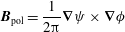 $$\begin{eqnarray}\boldsymbol{B}_{\text{pol}}=\frac{1}{2\unicode[STIX]{x03C0}}\unicode[STIX]{x1D735}\unicode[STIX]{x1D713}\times \unicode[STIX]{x1D735}\unicode[STIX]{x1D719}\end{eqnarray}$$
and the toroidal field is
 $$\begin{eqnarray}\boldsymbol{B}_{\text{tor}}=\frac{\unicode[STIX]{x1D707}_{0}I}{2\unicode[STIX]{x03C0}}\unicode[STIX]{x1D735}\unicode[STIX]{x1D719}.\end{eqnarray}$$
The poloidal flux
 $\unicode[STIX]{x1D713}$
and the poloidal current
$\unicode[STIX]{x1D713}$
and the poloidal current
 $I$
are defined as
$I$
are defined as
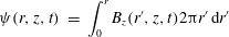 $$\begin{eqnarray}\displaystyle \unicode[STIX]{x1D713}(r,z,t) & = & \displaystyle \int _{0}^{r}B_{z}(r^{\prime },z,t)2\unicode[STIX]{x03C0}r^{\prime }\,\text{d}r^{\prime }\end{eqnarray}$$
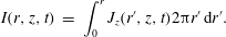 $$\begin{eqnarray}\displaystyle I(r,z,t) & = & \displaystyle \int _{0}^{r}J_{z}(r^{\prime },z,t)2\unicode[STIX]{x03C0}r^{\prime }\,\text{d}r^{\prime }.\end{eqnarray}$$
 $I$
and
$I$
and
 $\unicode[STIX]{x1D713}$
are respectively the electric current and magnetic flux passing through a circle of radius
$\unicode[STIX]{x1D713}$
are respectively the electric current and magnetic flux passing through a circle of radius
 $r$
at axial location
$r$
at axial location
 $z$
at time
$z$
at time
 $t$
. From Ampere’s law
$t$
. From Ampere’s law
 $\unicode[STIX]{x1D735}\times \boldsymbol{B}=\unicode[STIX]{x1D707}_{0}\boldsymbol{J}$
the poloidal and toroidal current densities are
$\unicode[STIX]{x1D735}\times \boldsymbol{B}=\unicode[STIX]{x1D707}_{0}\boldsymbol{J}$
the poloidal and toroidal current densities are 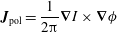 $$\begin{eqnarray}\boldsymbol{J}_{\text{pol}}=\frac{1}{2\unicode[STIX]{x03C0}}\unicode[STIX]{x1D735}I\times \unicode[STIX]{x1D735}\unicode[STIX]{x1D719}\end{eqnarray}$$
and
 $$\begin{eqnarray}\boldsymbol{J}_{\text{tor}}=-\frac{r^{2}}{2\unicode[STIX]{x03C0}\unicode[STIX]{x1D707}_{0}}\left[\unicode[STIX]{x1D735}\boldsymbol{\cdot }\left(\frac{1}{r^{2}}\unicode[STIX]{x1D735}\unicode[STIX]{x1D713}\right)\right]\unicode[STIX]{x1D735}\unicode[STIX]{x1D719}.\end{eqnarray}$$
2.7 Equation of motion in terms of flux functions
As shown in Bellan (Reference Bellan2017, Reference Bellan2018a
) by expanding the convective term
 $\boldsymbol{U}\boldsymbol{\cdot }\unicode[STIX]{x1D735}\boldsymbol{U}$
on the left-hand side of the MHD equation of motion (2.1) and also using (2.19), (2.20), (2.22) and (2.23) to express the
$\boldsymbol{U}\boldsymbol{\cdot }\unicode[STIX]{x1D735}\boldsymbol{U}$
on the left-hand side of the MHD equation of motion (2.1) and also using (2.19), (2.20), (2.22) and (2.23) to express the
 $\boldsymbol{J}\times \boldsymbol{B}$
term on the right-hand side, the radial, toroidal and axial components of the MHD equation of motion can be expressed without approximation as
$\boldsymbol{J}\times \boldsymbol{B}$
term on the right-hand side, the radial, toroidal and axial components of the MHD equation of motion can be expressed without approximation as
 $$\begin{eqnarray}\displaystyle \frac{\unicode[STIX]{x2202}}{\unicode[STIX]{x2202}t}(\unicode[STIX]{x1D70C}U_{r})+\unicode[STIX]{x1D735}\boldsymbol{\cdot }(\unicode[STIX]{x1D70C}U_{r}\boldsymbol{U}) & = & \displaystyle \frac{1}{4\unicode[STIX]{x03C0}^{2}}\left(-\frac{1}{\unicode[STIX]{x1D707}_{0}}\frac{\unicode[STIX]{x2202}\unicode[STIX]{x1D713}}{\unicode[STIX]{x2202}r}\unicode[STIX]{x1D735}\boldsymbol{\cdot }\left(\frac{1}{r^{2}}\unicode[STIX]{x1D735}\unicode[STIX]{x1D713}\right)-\frac{\unicode[STIX]{x1D707}_{0}I}{r^{2}}\frac{\unicode[STIX]{x2202}I}{\unicode[STIX]{x2202}r}\right)-\frac{\unicode[STIX]{x2202}P}{\unicode[STIX]{x2202}r}+\frac{\unicode[STIX]{x1D70C}U_{\unicode[STIX]{x1D719}}^{2}}{r}\nonumber\\ \displaystyle & & \displaystyle\end{eqnarray}$$
 $$\begin{eqnarray}\displaystyle \frac{\unicode[STIX]{x2202}}{\unicode[STIX]{x2202}t}(\unicode[STIX]{x1D70C}rU_{\unicode[STIX]{x1D719}})+\unicode[STIX]{x1D735}\boldsymbol{\cdot }(\unicode[STIX]{x1D70C}rU_{\unicode[STIX]{x1D719}}\boldsymbol{U}) & = & \displaystyle \frac{1}{4\unicode[STIX]{x03C0}^{2}}(\unicode[STIX]{x1D735}I\times \unicode[STIX]{x1D735}\unicode[STIX]{x1D713}\boldsymbol{\cdot }\unicode[STIX]{x1D735}\unicode[STIX]{x1D719})\end{eqnarray}$$
 $$\begin{eqnarray}\displaystyle \frac{\unicode[STIX]{x2202}}{\unicode[STIX]{x2202}t}(\unicode[STIX]{x1D70C}U_{z})+\unicode[STIX]{x1D735}\boldsymbol{\cdot }(\unicode[STIX]{x1D70C}U_{z}\boldsymbol{U}) & = & \displaystyle \frac{1}{4\unicode[STIX]{x03C0}^{2}}\left(-\frac{1}{\unicode[STIX]{x1D707}_{0}}\frac{\unicode[STIX]{x2202}\unicode[STIX]{x1D713}}{\unicode[STIX]{x2202}z}\unicode[STIX]{x1D735}\boldsymbol{\cdot }\left(\frac{1}{r^{2}}\unicode[STIX]{x1D735}\unicode[STIX]{x1D713}\right)-\frac{\unicode[STIX]{x1D707}_{0}I}{r^{2}}\frac{\unicode[STIX]{x2202}I}{\unicode[STIX]{x2202}z}\right)-\frac{\unicode[STIX]{x2202}P}{\unicode[STIX]{x2202}z}.\qquad\end{eqnarray}$$
 $\boldsymbol{J}\times \boldsymbol{B}$
, the radial component of the pressure gradient and centrifugal force. Equation (2.24b
), the toroidal component of the equation of motion, contains on its right-hand side only the toroidal component of
$\boldsymbol{J}\times \boldsymbol{B}$
, the radial component of the pressure gradient and centrifugal force. Equation (2.24b
), the toroidal component of the equation of motion, contains on its right-hand side only the toroidal component of
 $\boldsymbol{J}\times \boldsymbol{B}$
as axisymmetry prevents the pressure gradient from having a toroidal component. Equation (2.24c
), the axial component of the equation of motion, contains on its right-hand side the axial component of
$\boldsymbol{J}\times \boldsymbol{B}$
as axisymmetry prevents the pressure gradient from having a toroidal component. Equation (2.24c
), the axial component of the equation of motion, contains on its right-hand side the axial component of
 $\boldsymbol{J}\times \boldsymbol{B}$
and the axial component of the pressure gradient. The peculiar form of the Laplacian-like term
$\boldsymbol{J}\times \boldsymbol{B}$
and the axial component of the pressure gradient. The peculiar form of the Laplacian-like term  $$\begin{eqnarray}\unicode[STIX]{x1D735}\boldsymbol{\cdot }\left(\frac{1}{r^{2}}\unicode[STIX]{x1D735}\unicode[STIX]{x1D713}\right)=\frac{1}{r^{2}}\left(r\frac{\unicode[STIX]{x2202}}{\unicode[STIX]{x2202}r}\left(\frac{1}{r}\frac{\unicode[STIX]{x2202}\unicode[STIX]{x1D713}}{\unicode[STIX]{x2202}r}\right)+\frac{\unicode[STIX]{x2202}^{2}\unicode[STIX]{x1D713}}{\unicode[STIX]{x2202}z^{2}}\right)\end{eqnarray}$$
means that this term becomes relatively unimportant compared to the other terms if
 $\unicode[STIX]{x1D713}\sim r^{2}$
. This is for two reasons: first, the contribution involving
$\unicode[STIX]{x1D713}\sim r^{2}$
. This is for two reasons: first, the contribution involving
 $r^{-1}\unicode[STIX]{x2202}/\unicode[STIX]{x2202}r(r^{2})$
is a constant so the next
$r^{-1}\unicode[STIX]{x2202}/\unicode[STIX]{x2202}r(r^{2})$
is a constant so the next
 $r$
derivative vanishes and second, because the jet by assumption is very long, the dependence on
$r$
derivative vanishes and second, because the jet by assumption is very long, the dependence on
 $z$
is weak.
$z$
is weak.
Ideal MHD presumes that particles make many cyclotron orbits between collisions in which case the microscopic particle behaviour is essentially governed by single-particle Hamiltonian Lagrangian theory. This theory prescribes angular motion in terms of the canonical angular momentum
 $P_{\unicode[STIX]{x1D719}}=mrv_{\unicode[STIX]{x1D719}}+qrA_{\unicode[STIX]{x1D719}}$
and shows that because of the assumed axisymmetry, the canonical angular momentum of a particle is an exact constant of the motion, i.e.
$P_{\unicode[STIX]{x1D719}}=mrv_{\unicode[STIX]{x1D719}}+qrA_{\unicode[STIX]{x1D719}}$
and shows that because of the assumed axisymmetry, the canonical angular momentum of a particle is an exact constant of the motion, i.e.
 $$\begin{eqnarray}P_{\unicode[STIX]{x1D719}}=mrv_{\unicode[STIX]{x1D719}}+\frac{1}{2\unicode[STIX]{x03C0}}q\unicode[STIX]{x1D713}(r,z,t)=\text{const}.\end{eqnarray}$$
Here we have used
 $\boldsymbol{B}_{\text{pol}}=\unicode[STIX]{x1D735}\times ((2\unicode[STIX]{x03C0}r)^{-1}\unicode[STIX]{x1D713}\hat{\unicode[STIX]{x1D719}})=\unicode[STIX]{x1D735}\times (A_{\unicode[STIX]{x1D719}}\hat{\unicode[STIX]{x1D719}})$
to give
$\boldsymbol{B}_{\text{pol}}=\unicode[STIX]{x1D735}\times ((2\unicode[STIX]{x03C0}r)^{-1}\unicode[STIX]{x1D713}\hat{\unicode[STIX]{x1D719}})=\unicode[STIX]{x1D735}\times (A_{\unicode[STIX]{x1D719}}\hat{\unicode[STIX]{x1D719}})$
to give
 $\unicode[STIX]{x1D713}(r,z,t)=2\unicode[STIX]{x03C0}rA_{\unicode[STIX]{x1D719}}(r,z,t)$
. A zero-mass particle would thus have to stay on a surface of constant poloidal flux. If finite particle mass is taken into account (2.26) implies that
$\unicode[STIX]{x1D713}(r,z,t)=2\unicode[STIX]{x03C0}rA_{\unicode[STIX]{x1D719}}(r,z,t)$
. A zero-mass particle would thus have to stay on a surface of constant poloidal flux. If finite particle mass is taken into account (2.26) implies that
 $\unicode[STIX]{x1D6FF}P_{\unicode[STIX]{x1D719}}=0$
so
$\unicode[STIX]{x1D6FF}P_{\unicode[STIX]{x1D719}}=0$
so
 $$\begin{eqnarray}\unicode[STIX]{x1D6FF}\left(mrv_{\unicode[STIX]{x1D719}}+\frac{1}{2\unicode[STIX]{x03C0}}q\unicode[STIX]{x1D713}(r,z,t)\right)=mr\unicode[STIX]{x1D6FF}v_{\unicode[STIX]{x1D719}}+mv_{\unicode[STIX]{x1D719}}\unicode[STIX]{x1D6FF}r+\frac{q}{2\unicode[STIX]{x03C0}}\left(\unicode[STIX]{x1D6FF}r\frac{\unicode[STIX]{x2202}\unicode[STIX]{x1D713}}{\unicode[STIX]{x2202}r}+\unicode[STIX]{x1D6FF}z\frac{\unicode[STIX]{x2202}\unicode[STIX]{x1D713}}{\unicode[STIX]{x2202}z}+\unicode[STIX]{x1D6FF}t\frac{\unicode[STIX]{x2202}\unicode[STIX]{x1D713}}{\unicode[STIX]{x2202}t}\right)=0.\end{eqnarray}$$
Since Faraday’s law implies
 $$\begin{eqnarray}E_{\unicode[STIX]{x1D719}}=-\frac{\unicode[STIX]{x2202}A_{\unicode[STIX]{x1D719}}}{\unicode[STIX]{x2202}t}=-\frac{1}{2\unicode[STIX]{x03C0}r}\frac{\unicode[STIX]{x2202}\unicode[STIX]{x1D713}}{\unicode[STIX]{x2202}t}\end{eqnarray}$$
and (2.19) gives
 $$\begin{eqnarray}\displaystyle B_{r} & = & \displaystyle -\frac{1}{2\unicode[STIX]{x03C0}r}\frac{\unicode[STIX]{x2202}\unicode[STIX]{x1D713}}{\unicode[STIX]{x2202}z}\end{eqnarray}$$
 $$\begin{eqnarray}\displaystyle B_{z} & = & \displaystyle \frac{1}{2\unicode[STIX]{x03C0}r}\frac{\unicode[STIX]{x2202}\unicode[STIX]{x1D713}}{\unicode[STIX]{x2202}r}\end{eqnarray}$$
 $$\begin{eqnarray}\unicode[STIX]{x1D6FF}v_{\unicode[STIX]{x1D719}}+\dot{\unicode[STIX]{x1D719}}\unicode[STIX]{x1D6FF}r-\hat{\unicode[STIX]{x1D719}}\boldsymbol{\cdot }(\hat{r}\unicode[STIX]{x1D6FF}r+\hat{z}\unicode[STIX]{x1D6FF}z)\times \frac{q}{m}\boldsymbol{B}_{\text{pol}}-\frac{q}{m}\unicode[STIX]{x1D6FF}tE_{\unicode[STIX]{x1D719}}=0.\end{eqnarray}$$
The term containing
 $E_{\unicode[STIX]{x1D719}}$
results from motion of the flux surface and so for purposes of calculating displacement from a flux surface, we may assume that the flux surface is stationary so
$E_{\unicode[STIX]{x1D719}}$
results from motion of the flux surface and so for purposes of calculating displacement from a flux surface, we may assume that the flux surface is stationary so
 $E_{\unicode[STIX]{x1D719}}=0$
. If a particle is assumed to be making cyclotron orbits with superimposed particle drifts as dictated by guiding centre theory, then
$E_{\unicode[STIX]{x1D719}}=0$
. If a particle is assumed to be making cyclotron orbits with superimposed particle drifts as dictated by guiding centre theory, then
 $r\dot{\unicode[STIX]{x1D719}}$
is of the order of or smaller than the thermal velocity, as is
$r\dot{\unicode[STIX]{x1D719}}$
is of the order of or smaller than the thermal velocity, as is
 $\unicode[STIX]{x1D6FF}v_{\unicode[STIX]{x1D719}}$
. The maximum deviation that a particle can make from its original position on a flux surface is then
$\unicode[STIX]{x1D6FF}v_{\unicode[STIX]{x1D719}}$
. The maximum deviation that a particle can make from its original position on a flux surface is then
 $$\begin{eqnarray}(\hat{r}\unicode[STIX]{x1D6FF}r+\hat{z}\unicode[STIX]{x1D6FF}z)_{\max }\simeq \frac{v_{T}}{qB_{\text{pol}}/m}\end{eqnarray}$$
which is a Larmor radius calculated using the poloidal field only. If charged particles cannot move more than a poloidal Larmor radius away from the poloidal flux surface on which they originate, then it would be impossible to have a steady-state electric current flowing perpendicular to poloidal flux surfaces. Thus, any steady-state electric current must flow on a poloidal flux surface. When collisions are taken into account it is seen that the perpendicular resistivity is much higher than the parallel resistivity, showing that there is negligible current across flux surfaces since such a current would be perpendicular to the magnetic field.
If the poloidal current flows on poloidal flux surfaces, then
 $I=I(\unicode[STIX]{x1D713})$
so
$I=I(\unicode[STIX]{x1D713})$
so
 $\unicode[STIX]{x1D735}I=(\unicode[STIX]{x2202}I/\unicode[STIX]{x2202}\unicode[STIX]{x1D713})\unicode[STIX]{x1D735}\unicode[STIX]{x1D713}$
in which case the right-hand side of (2.24b
) vanishes. We note that if the poloidal current were to flow across poloidal flux surfaces, then
$\unicode[STIX]{x1D735}I=(\unicode[STIX]{x2202}I/\unicode[STIX]{x2202}\unicode[STIX]{x1D713})\unicode[STIX]{x1D735}\unicode[STIX]{x1D713}$
in which case the right-hand side of (2.24b
) vanishes. We note that if the poloidal current were to flow across poloidal flux surfaces, then
 $\unicode[STIX]{x1D735}I\times \unicode[STIX]{x1D735}\unicode[STIX]{x1D713}\boldsymbol{\cdot }\unicode[STIX]{x1D735}\unicode[STIX]{x1D719}$
would be finite which would constitute a torque that changes the angular momentum density
$\unicode[STIX]{x1D735}I\times \unicode[STIX]{x1D735}\unicode[STIX]{x1D713}\boldsymbol{\cdot }\unicode[STIX]{x1D735}\unicode[STIX]{x1D719}$
would be finite which would constitute a torque that changes the angular momentum density
 $\unicode[STIX]{x1D70C}rU_{\unicode[STIX]{x1D719}}$
. The confinement of both signs of particles to the vicinity of poloidal flux surfaces means that there can be no electric current across poloidal flux surfaces; this implies that
$\unicode[STIX]{x1D70C}rU_{\unicode[STIX]{x1D719}}$
. The confinement of both signs of particles to the vicinity of poloidal flux surfaces means that there can be no electric current across poloidal flux surfaces; this implies that
 $\unicode[STIX]{x1D735}I\times \unicode[STIX]{x1D735}\unicode[STIX]{x1D713}\boldsymbol{\cdot }\unicode[STIX]{x1D735}\unicode[STIX]{x1D719}$
must vanish in steady state. It is possible however to have a transient finite
$\unicode[STIX]{x1D735}I\times \unicode[STIX]{x1D735}\unicode[STIX]{x1D713}\boldsymbol{\cdot }\unicode[STIX]{x1D735}\unicode[STIX]{x1D719}$
must vanish in steady state. It is possible however to have a transient finite
 $\unicode[STIX]{x1D735}I\times \unicode[STIX]{x1D735}\unicode[STIX]{x1D713}\boldsymbol{\cdot }\unicode[STIX]{x1D735}\unicode[STIX]{x1D719}$
. Such a situation corresponds to the transient current that results when particles make inward or outward transient displacements from the poloidal flux surface. Because of the dependence on charge sign in (2.31), ions and electrons displace in opposite directions and this corresponds to a transient current normal to the flux surface. These transient currents provide a transient torque that rotates the plasma by a finite amount so that the plasma twists up. This twisting is in the same fashion as the twisting of the magnetic field when the poloidal current is ramped up (Bellan Reference Bellan2003). This means that if the jet starts with
$\unicode[STIX]{x1D735}I\times \unicode[STIX]{x1D735}\unicode[STIX]{x1D713}\boldsymbol{\cdot }\unicode[STIX]{x1D735}\unicode[STIX]{x1D719}$
. Such a situation corresponds to the transient current that results when particles make inward or outward transient displacements from the poloidal flux surface. Because of the dependence on charge sign in (2.31), ions and electrons displace in opposite directions and this corresponds to a transient current normal to the flux surface. These transient currents provide a transient torque that rotates the plasma by a finite amount so that the plasma twists up. This twisting is in the same fashion as the twisting of the magnetic field when the poloidal current is ramped up (Bellan Reference Bellan2003). This means that if the jet starts with
 $U_{\unicode[STIX]{x1D719}}=0$
it will have
$U_{\unicode[STIX]{x1D719}}=0$
it will have
 $U_{\unicode[STIX]{x1D719}}=0$
at later times except for times when the current is changing and the amount of field twist is changing.
$U_{\unicode[STIX]{x1D719}}=0$
at later times except for times when the current is changing and the amount of field twist is changing.
The jet main column flows primarily in the
 $z$
direction so
$z$
direction so
 $U_{r}\ll U_{z}$
. Thus, in the main column terms involving
$U_{r}\ll U_{z}$
. Thus, in the main column terms involving
 $U_{r}$
,
$U_{r}$
,
 $U_{\unicode[STIX]{x1D719}}$
and
$U_{\unicode[STIX]{x1D719}}$
and
 $\unicode[STIX]{x1D735}\boldsymbol{\cdot }(r^{-2}\unicode[STIX]{x1D735}\unicode[STIX]{x1D713})$
may be dropped. Furthermore, all terms in (2.24b
) vanish. Equation (2.24a
) then reduces to the Bennett pinch relation
$\unicode[STIX]{x1D735}\boldsymbol{\cdot }(r^{-2}\unicode[STIX]{x1D735}\unicode[STIX]{x1D713})$
may be dropped. Furthermore, all terms in (2.24b
) vanish. Equation (2.24a
) then reduces to the Bennett pinch relation
 $$\begin{eqnarray}\frac{\unicode[STIX]{x2202}P}{\unicode[STIX]{x2202}r}=-\frac{1}{4\unicode[STIX]{x03C0}^{2}}\left(\frac{\unicode[STIX]{x1D707}_{0}I}{r^{2}}\frac{\unicode[STIX]{x2202}I}{\unicode[STIX]{x2202}r}\right),\end{eqnarray}$$
which is the balancing of the outward force from the pressure by the inward pinch force
 $-J_{z}B_{\unicode[STIX]{x1D719}}$
. The pinching corresponds to the red circles in figure 1 behaving like circular elastic bands trying to reduce their radii and so providing a radial inward force. The simplest non-trivial situation where
$-J_{z}B_{\unicode[STIX]{x1D719}}$
. The pinching corresponds to the red circles in figure 1 behaving like circular elastic bands trying to reduce their radii and so providing a radial inward force. The simplest non-trivial situation where
 $I=I(\unicode[STIX]{x1D713})$
is where
$I=I(\unicode[STIX]{x1D713})$
is where
 $I$
is a linear function of
$I$
is a linear function of
 $\unicode[STIX]{x1D713}$
and so it is convenient to assume that
$\unicode[STIX]{x1D713}$
and so it is convenient to assume that
 $$\begin{eqnarray}\unicode[STIX]{x1D707}_{0}I=\unicode[STIX]{x1D706}\unicode[STIX]{x1D713},\end{eqnarray}$$
where
 $\unicode[STIX]{x1D706}$
is a constant having dimensions of inverse length. Equation (2.33) is then similar to the self-organized Taylor state discussed in § 2.4, the difference being that here
$\unicode[STIX]{x1D706}$
is a constant having dimensions of inverse length. Equation (2.33) is then similar to the self-organized Taylor state discussed in § 2.4, the difference being that here
 $\unicode[STIX]{x1D6FD}$
is not assumed to be zero and the configuration is not assumed to be in equilibrium. From a mathematical point of view this means that (2.15a
) and (2.15c
) are satisfied but not (2.15b
) because to the extent that
$\unicode[STIX]{x1D6FD}$
is not assumed to be zero and the configuration is not assumed to be in equilibrium. From a mathematical point of view this means that (2.15a
) and (2.15c
) are satisfied but not (2.15b
) because to the extent that
 $B_{z}$
is uniform,
$B_{z}$
is uniform,
 $J_{\unicode[STIX]{x1D719}}$
is zero and to the extent that
$J_{\unicode[STIX]{x1D719}}$
is zero and to the extent that
 $P$
is finite,
$P$
is finite,
 $B_{\unicode[STIX]{x1D719}}$
is finite. As discussed in Lewis & Bellan (Reference Lewis and Bellan1990), for reasons of mathematical regularity each of
$B_{\unicode[STIX]{x1D719}}$
is finite. As discussed in Lewis & Bellan (Reference Lewis and Bellan1990), for reasons of mathematical regularity each of
 $I$
and
$I$
and
 $\unicode[STIX]{x1D713}$
at small
$\unicode[STIX]{x1D713}$
at small
 $r$
(i.e. near the jet axis) must be proportional to
$r$
(i.e. near the jet axis) must be proportional to
 $r^{2}$
if the axial magnetic field and axial current density are finite on axis. Thus, at small
$r^{2}$
if the axial magnetic field and axial current density are finite on axis. Thus, at small
 $r$
(2.33) must be almost exactly true and not just the simplest non-trivial situation.
$r$
(2.33) must be almost exactly true and not just the simplest non-trivial situation.
The simplest non-trivial form for
 $\unicode[STIX]{x1D713}$
in the jet main column is
$\unicode[STIX]{x1D713}$
in the jet main column is
 $$\begin{eqnarray}\unicode[STIX]{x1D713}=\unicode[STIX]{x1D713}_{0}\frac{r^{2}}{a^{2}},\end{eqnarray}$$
where
 $a$
is the jet radius; equation (2.29b
) shows this form for
$a$
is the jet radius; equation (2.29b
) shows this form for
 $\unicode[STIX]{x1D713}$
corresponds to a uniform axial magnetic field in the jet main column. Equation (2.32) can then be integrated to give
$\unicode[STIX]{x1D713}$
corresponds to a uniform axial magnetic field in the jet main column. Equation (2.32) can then be integrated to give
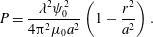 $$\begin{eqnarray}P=\frac{\unicode[STIX]{x1D706}^{2}\unicode[STIX]{x1D713}_{0}^{2}}{4\unicode[STIX]{x03C0}^{2}\unicode[STIX]{x1D707}_{0}a^{2}}\left(1-\frac{r^{2}}{a^{2}}\right).\end{eqnarray}$$
If
 $a$
is allowed to have a weak dependence on
$a$
is allowed to have a weak dependence on
 $z$
this generalizes to
$z$
this generalizes to
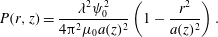 $$\begin{eqnarray}P(r,z)=\frac{\unicode[STIX]{x1D706}^{2}\unicode[STIX]{x1D713}_{0}^{2}}{4\unicode[STIX]{x03C0}^{2}\unicode[STIX]{x1D707}_{0}a(z)^{2}}\left(1-\frac{r^{2}}{a(z)^{2}}\right).\end{eqnarray}$$
Comparison of (2.35) and (2.36) shows that if
 $a$
does depend on
$a$
does depend on
 $z$
there will then be a pressure gradient in the the
$z$
there will then be a pressure gradient in the the
 $z$
direction and
$z$
direction and
 $\unicode[STIX]{x2202}P/\unicode[STIX]{x2202}z$
will be proportional to
$\unicode[STIX]{x2202}P/\unicode[STIX]{x2202}z$
will be proportional to
 $\unicode[STIX]{x2202}a/\unicode[STIX]{x2202}z$
. The pressure gradient is such as to accelerate plasma axially from where
$\unicode[STIX]{x2202}a/\unicode[STIX]{x2202}z$
. The pressure gradient is such as to accelerate plasma axially from where
 $a$
is small to where
$a$
is small to where
 $a$
is large.
$a$
is large.
We now turn attention to (2.24c
) and assume a quasi-steady behaviour so the term containing
 $\unicode[STIX]{x2202}/\unicode[STIX]{x2202}t$
is small compared to the other terms. Because
$\unicode[STIX]{x2202}/\unicode[STIX]{x2202}t$
is small compared to the other terms. Because
 $U_{r}\ll U_{z}$
in the main column and
$U_{r}\ll U_{z}$
in the main column and
 $\unicode[STIX]{x1D735}\boldsymbol{\cdot }(r^{-2}\unicode[STIX]{x1D735}\unicode[STIX]{x1D713})$
is small compared to the other terms, this equation reduces to
$\unicode[STIX]{x1D735}\boldsymbol{\cdot }(r^{-2}\unicode[STIX]{x1D735}\unicode[STIX]{x1D713})$
is small compared to the other terms, this equation reduces to
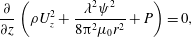 $$\begin{eqnarray}\frac{\unicode[STIX]{x2202}}{\unicode[STIX]{x2202}z}\left(\unicode[STIX]{x1D70C}U_{z}^{2}+\frac{\unicode[STIX]{x1D706}^{2}\unicode[STIX]{x1D713}^{2}}{8\unicode[STIX]{x03C0}^{2}\unicode[STIX]{x1D707}_{0}r^{2}}+P\right)=0,\end{eqnarray}$$
where (2.33) has been used. Equation (2.37) is a generalized Bernoulli relation and upon substituting (2.34) and (2.36) becomes
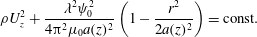 $$\begin{eqnarray}\unicode[STIX]{x1D70C}U_{z}^{2}+\frac{\unicode[STIX]{x1D706}^{2}\unicode[STIX]{x1D713}_{0}^{2}}{4\unicode[STIX]{x03C0}^{2}\unicode[STIX]{x1D707}_{0}a(z)^{2}}\left(1-\frac{r^{2}}{2a(z)^{2}}\right)=\text{const}.\end{eqnarray}$$
On the
 $z$
axis where
$z$
axis where
 $r=0$
the constant can be evaluated at
$r=0$
the constant can be evaluated at
 $z=0$
where
$z=0$
where
 $U_{z}\simeq 0$
and
$U_{z}\simeq 0$
and
 $a(z)$
is small and then also evaluated just before the jet tip at approximately
$a(z)$
is small and then also evaluated just before the jet tip at approximately
 $z=l$
where
$z=l$
where
 $a(z)$
is large and
$a(z)$
is large and
 $U_{z}$
is large. This gives
$U_{z}$
is large. This gives
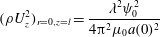 $$\begin{eqnarray}(\unicode[STIX]{x1D70C}U_{z}^{2})_{r=0,z=l}=\frac{\unicode[STIX]{x1D706}^{2}\unicode[STIX]{x1D713}_{0}^{2}}{4\unicode[STIX]{x03C0}^{2}\unicode[STIX]{x1D707}_{0}a(0)^{2}}\end{eqnarray}$$
so
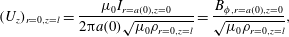 $$\begin{eqnarray}(U_{z})_{r=0,z=l}=\frac{\unicode[STIX]{x1D707}_{0}I_{r=a(0),z=0}}{2\unicode[STIX]{x03C0}a(0)\sqrt{\unicode[STIX]{x1D707}_{0}\unicode[STIX]{x1D70C}_{r=0,z=l}}}=\frac{B_{\unicode[STIX]{x1D719},r=a(0),z=0}}{\sqrt{\unicode[STIX]{x1D707}_{0}\unicode[STIX]{x1D70C}_{r=0,z=l}}},\end{eqnarray}$$
which scales like an Alfvén velocity yet is not the local Alfvén velocity because
 $B_{\unicode[STIX]{x1D719}}$
is not the entire magnetic field and furthermore
$B_{\unicode[STIX]{x1D719}}$
is not the entire magnetic field and furthermore
 $B_{\unicode[STIX]{x1D719}}$
is evaluated at a location different from where the velocity is being determined. Equation (2.40) shows that the jet velocity is linearly proportional to the poloidal current.
$B_{\unicode[STIX]{x1D719}}$
is evaluated at a location different from where the velocity is being determined. Equation (2.40) shows that the jet velocity is linearly proportional to the poloidal current.
The constant in (2.38) will be smaller off the
 $z$
-axis and so the general form of the velocity will be
$z$
-axis and so the general form of the velocity will be
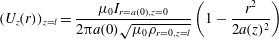 $$\begin{eqnarray}(U_{z}(r))_{z=l}=\frac{\unicode[STIX]{x1D707}_{0}I_{r=a(0),z=0}}{2\unicode[STIX]{x03C0}a(0)\sqrt{\unicode[STIX]{x1D707}_{0}\unicode[STIX]{x1D70C}_{r=0,z=l}}}\left(1-\frac{r^{2}}{2a(z)^{2}}\right)\end{eqnarray}$$
indicating there is a shearing of the axial velocity with the peak axial velocity located on the
 $z$
-axis. The axial gradient of the middle term in (2.37) corresponds to the dominant part of the axial component of the
$z$
-axis. The axial gradient of the middle term in (2.37) corresponds to the dominant part of the axial component of the
 $\boldsymbol{J}\times \boldsymbol{B}$
force, i.e. to
$\boldsymbol{J}\times \boldsymbol{B}$
force, i.e. to
 $J_{r}B_{\unicode[STIX]{x1D719}}=-\unicode[STIX]{x2202}/\unicode[STIX]{x2202}z(B_{\unicode[STIX]{x1D719}}^{2}/2\unicode[STIX]{x1D707}_{0})$
since
$J_{r}B_{\unicode[STIX]{x1D719}}=-\unicode[STIX]{x2202}/\unicode[STIX]{x2202}z(B_{\unicode[STIX]{x1D719}}^{2}/2\unicode[STIX]{x1D707}_{0})$
since
 $B_{\unicode[STIX]{x1D719}}=\unicode[STIX]{x1D707}_{0}I/2\unicode[STIX]{x03C0}r$
and
$B_{\unicode[STIX]{x1D719}}=\unicode[STIX]{x1D707}_{0}I/2\unicode[STIX]{x03C0}r$
and
 $\unicode[STIX]{x1D707}_{0}I=\unicode[STIX]{x1D706}\unicode[STIX]{x1D713}$
. Because
$\unicode[STIX]{x1D707}_{0}I=\unicode[STIX]{x1D706}\unicode[STIX]{x1D713}$
. Because
 $\unicode[STIX]{x1D713}\sim r^{2}$
this contribution to the axial force vanishes on the
$\unicode[STIX]{x1D713}\sim r^{2}$
this contribution to the axial force vanishes on the
 $z$
-axis so on the
$z$
-axis so on the
 $z$
-axis the axial force is entirely the result of the axial pressure gradient. This axial force
$z$
-axis the axial force is entirely the result of the axial pressure gradient. This axial force
 $-\unicode[STIX]{x2202}/\unicode[STIX]{x2202}z(B_{\unicode[STIX]{x1D719}}^{2}/2\unicode[STIX]{x1D707}_{0})$
is shown in figure 1 as the red circles pushing up from where they are densely packed and so constituting an axial upward force acting on the main column.
$-\unicode[STIX]{x2202}/\unicode[STIX]{x2202}z(B_{\unicode[STIX]{x1D719}}^{2}/2\unicode[STIX]{x1D707}_{0})$
is shown in figure 1 as the red circles pushing up from where they are densely packed and so constituting an axial upward force acting on the main column.
The expressions derived so far describe the jet main column. At the jet tip, the poloidal field bends around so it is no longer appropriate to assume that
 $\unicode[STIX]{x1D713}$
has a weak dependence on
$\unicode[STIX]{x1D713}$
has a weak dependence on
 $z$
. This bending implies existence of a substantial radial magnetic field
$z$
. This bending implies existence of a substantial radial magnetic field
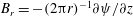 $B_{r}=-(2\unicode[STIX]{x03C0}r)^{-1}\unicode[STIX]{x2202}\unicode[STIX]{x1D713}/\unicode[STIX]{x2202}z$
. The suddenness of the bending implies a toroidal current
$B_{r}=-(2\unicode[STIX]{x03C0}r)^{-1}\unicode[STIX]{x2202}\unicode[STIX]{x1D713}/\unicode[STIX]{x2202}z$
. The suddenness of the bending implies a toroidal current
 $J_{\unicode[STIX]{x1D719}}=\unicode[STIX]{x1D707}_{0}^{-1}\unicode[STIX]{x2202}B_{r}/\unicode[STIX]{x2202}z$
. Both
$J_{\unicode[STIX]{x1D719}}=\unicode[STIX]{x1D707}_{0}^{-1}\unicode[STIX]{x2202}B_{r}/\unicode[STIX]{x2202}z$
. Both
 $B_{r}$
and
$B_{r}$
and
 $J_{\unicode[STIX]{x1D719}}$
are positive so they combine to give a retarding axial force
$J_{\unicode[STIX]{x1D719}}$
are positive so they combine to give a retarding axial force
 $-J_{\unicode[STIX]{x1D719}}B_{r}$
. The bending of the poloidal field and the retarding force at the tip are sketched in figure 1. This retarding force means that the jet tip velocity will be somewhat slower than that of the jet main column so the jet main column continuously piles up (stagnates) at the tip. An observer moving with the jet and located where the jet main column is catching up with the tip would see a converging flow since the observer is moving slower than the main column but faster than the tip. This flow convergence in the jet frame produces a density pile-up. Since toroidal magnetic flux is frozen into the plasma, there will also be a pile-up of the frozen-in toroidal magnetic flux, i.e. an increase in the density of the toroidal magnetic flux. However, the density of toroidal magnetic flux is just the toroidal field and so this stagnation will increase the local toroidal magnetic field. Since the toroidal magnetic field is what produces the pinch force, the stagnation will increase the pinch force and so tend to collimate the jet. Thus, the jet is self-collimating and the collimation process is like a zipper acting on the inner part of the poloidal field lines.
$-J_{\unicode[STIX]{x1D719}}B_{r}$
. The bending of the poloidal field and the retarding force at the tip are sketched in figure 1. This retarding force means that the jet tip velocity will be somewhat slower than that of the jet main column so the jet main column continuously piles up (stagnates) at the tip. An observer moving with the jet and located where the jet main column is catching up with the tip would see a converging flow since the observer is moving slower than the main column but faster than the tip. This flow convergence in the jet frame produces a density pile-up. Since toroidal magnetic flux is frozen into the plasma, there will also be a pile-up of the frozen-in toroidal magnetic flux, i.e. an increase in the density of the toroidal magnetic flux. However, the density of toroidal magnetic flux is just the toroidal field and so this stagnation will increase the local toroidal magnetic field. Since the toroidal magnetic field is what produces the pinch force, the stagnation will increase the pinch force and so tend to collimate the jet. Thus, the jet is self-collimating and the collimation process is like a zipper acting on the inner part of the poloidal field lines.
This argument for collimation can be justified mathematically by dotting the induction equation, (2.2), with
 $\unicode[STIX]{x1D735}\unicode[STIX]{x1D719}$
to obtain
$\unicode[STIX]{x1D735}\unicode[STIX]{x1D719}$
to obtain
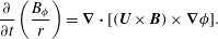 $$\begin{eqnarray}\frac{\unicode[STIX]{x2202}}{\unicode[STIX]{x2202}t}\left(\frac{B_{\unicode[STIX]{x1D719}}}{r}\right)=\unicode[STIX]{x1D735}\boldsymbol{\cdot }[(\boldsymbol{U}\times \boldsymbol{B})\times \unicode[STIX]{x1D735}\unicode[STIX]{x1D719}].\end{eqnarray}$$
Expanding the right-hand side gives
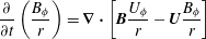 $$\begin{eqnarray}\frac{\unicode[STIX]{x2202}}{\unicode[STIX]{x2202}t}\left(\frac{B_{\unicode[STIX]{x1D719}}}{r}\right)=\unicode[STIX]{x1D735}\boldsymbol{\cdot }\left[\boldsymbol{B}\frac{U_{\unicode[STIX]{x1D719}}}{r}-\boldsymbol{U}\frac{B_{\unicode[STIX]{x1D719}}}{r}\right]\end{eqnarray}$$
or, on using
 $U_{\unicode[STIX]{x1D719}}=0$
,
$U_{\unicode[STIX]{x1D719}}=0$
,
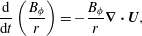 $$\begin{eqnarray}\frac{\text{d}}{\text{d}t}\left(\frac{B_{\unicode[STIX]{x1D719}}}{r}\right)=-\frac{B_{\unicode[STIX]{x1D719}}}{r}\unicode[STIX]{x1D735}\boldsymbol{\cdot }\boldsymbol{U},\end{eqnarray}$$
where
 $\text{d}/\text{d}t=\unicode[STIX]{x2202}/\unicode[STIX]{x2202}t+\boldsymbol{U}\boldsymbol{\cdot }\unicode[STIX]{x1D735}$
is the convective derivative, i.e. the derivative as seen by an observer moving with the jet. Equation (2.44) shows that
$\text{d}/\text{d}t=\unicode[STIX]{x2202}/\unicode[STIX]{x2202}t+\boldsymbol{U}\boldsymbol{\cdot }\unicode[STIX]{x1D735}$
is the convective derivative, i.e. the derivative as seen by an observer moving with the jet. Equation (2.44) shows that
 $B_{\unicode[STIX]{x1D719}}$
indeed increases in the jet frame where there is a converging flow, i.e. negative
$B_{\unicode[STIX]{x1D719}}$
indeed increases in the jet frame where there is a converging flow, i.e. negative
 $\unicode[STIX]{x1D735}\boldsymbol{\cdot }\boldsymbol{U}$
.
$\unicode[STIX]{x1D735}\boldsymbol{\cdot }\boldsymbol{U}$
.
Proceeding further, the equation of continuity, (2.3), can be written as
 $$\begin{eqnarray}\frac{\text{d}\unicode[STIX]{x1D70C}}{\text{d}t}+\unicode[STIX]{x1D70C}\unicode[STIX]{x1D735}\boldsymbol{\cdot }\boldsymbol{U}=0.\end{eqnarray}$$
Eliminating
 $\unicode[STIX]{x1D735}\boldsymbol{\cdot }\boldsymbol{U}$
between (2.44) and (2.45) gives
$\unicode[STIX]{x1D735}\boldsymbol{\cdot }\boldsymbol{U}$
between (2.44) and (2.45) gives
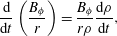 $$\begin{eqnarray}\frac{\text{d}}{\text{d}t}\left(\frac{B_{\unicode[STIX]{x1D719}}}{r}\right)=\frac{B_{\unicode[STIX]{x1D719}}}{r\unicode[STIX]{x1D70C}}\frac{\text{d}\unicode[STIX]{x1D70C}}{\text{d}t},\end{eqnarray}$$
which can be expressed as
 $$\begin{eqnarray}\frac{\text{d}}{\text{d}t}\ln \left(\frac{B_{\unicode[STIX]{x1D719}}}{\unicode[STIX]{x1D70C}r}\right)=0,\end{eqnarray}$$
which implies that
 $$\begin{eqnarray}\frac{B_{\unicode[STIX]{x1D719}}}{\unicode[STIX]{x1D70C}r}=\text{const. in the jet frame}.\end{eqnarray}$$
Thus, the increase in density that occurs as the main jet column stagnates at the tip will require a corresponding increase in
 $B_{\unicode[STIX]{x1D719}}/r$
. If
$B_{\unicode[STIX]{x1D719}}/r$
. If
 $r$
is set to be the jet radius
$r$
is set to be the jet radius
 $a(z)$
then since
$a(z)$
then since
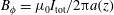 $B_{\unicode[STIX]{x1D719}}=\unicode[STIX]{x1D707}_{0}I_{\text{tot}}/2\unicode[STIX]{x03C0}a(z)$
where
$B_{\unicode[STIX]{x1D719}}=\unicode[STIX]{x1D707}_{0}I_{\text{tot}}/2\unicode[STIX]{x03C0}a(z)$
where
 $I_{\text{tot}}$
is the total poloidal current in the jet, it is seen that
$I_{\text{tot}}$
is the total poloidal current in the jet, it is seen that
 $a(z)$
must decrease if
$a(z)$
must decrease if
 $\unicode[STIX]{x1D70C}$
increases since
$\unicode[STIX]{x1D70C}$
increases since
 $I_{\text{tot}}$
is constant. This confirms the continuous self-collimation of the jet.
$I_{\text{tot}}$
is constant. This confirms the continuous self-collimation of the jet.
The relationship of the model presented here to that of Lynden-Bell can now be determined. Specifically, the magnetic tower model proposed by Lynden-Bell (Reference Lynden-Bell2003) corresponds to setting
 $\boldsymbol{U}=0$
,
$\boldsymbol{U}=0$
,
 $P=0$
, and
$P=0$
, and
 $I=I(\unicode[STIX]{x1D713})$
in (2.24a–c
) in which case
$I=I(\unicode[STIX]{x1D713})$
in (2.24a–c
) in which case
 $\unicode[STIX]{x1D735}I\times \unicode[STIX]{x1D735}\unicode[STIX]{x1D713}=0$
and so (2.24a
) and (
c
) reduce to
$\unicode[STIX]{x1D735}I\times \unicode[STIX]{x1D735}\unicode[STIX]{x1D713}=0$
and so (2.24a
) and (
c
) reduce to
 $$\begin{eqnarray}\displaystyle \frac{1}{\unicode[STIX]{x1D707}_{0}}\frac{\unicode[STIX]{x2202}\unicode[STIX]{x1D713}}{\unicode[STIX]{x2202}r}\unicode[STIX]{x1D735}\boldsymbol{\cdot }\left(\frac{1}{r^{2}}\unicode[STIX]{x1D735}\unicode[STIX]{x1D713}\right)+\frac{\unicode[STIX]{x1D707}_{0}I}{r^{2}}\frac{\unicode[STIX]{x2202}I}{\unicode[STIX]{x2202}r} & = & \displaystyle 0\end{eqnarray}$$
 $$\begin{eqnarray}\displaystyle \frac{1}{\unicode[STIX]{x1D707}_{0}}\frac{\unicode[STIX]{x2202}\unicode[STIX]{x1D713}}{\unicode[STIX]{x2202}z}\unicode[STIX]{x1D735}\boldsymbol{\cdot }\left(\frac{1}{r^{2}}\unicode[STIX]{x1D735}\unicode[STIX]{x1D713}\right)+\frac{\unicode[STIX]{x1D707}_{0}I}{r^{2}}\frac{\unicode[STIX]{x2202}I}{\unicode[STIX]{x2202}z} & = & \displaystyle 0.\end{eqnarray}$$
 $\unicode[STIX]{x2202}I/\unicode[STIX]{x2202}z=(\unicode[STIX]{x2202}I/\unicode[STIX]{x2202}\unicode[STIX]{x1D713})(\unicode[STIX]{x2202}\unicode[STIX]{x1D713}/\unicode[STIX]{x2202}z)$
and
$\unicode[STIX]{x2202}I/\unicode[STIX]{x2202}z=(\unicode[STIX]{x2202}I/\unicode[STIX]{x2202}\unicode[STIX]{x1D713})(\unicode[STIX]{x2202}\unicode[STIX]{x1D713}/\unicode[STIX]{x2202}z)$
and
 $\unicode[STIX]{x2202}I/\unicode[STIX]{x2202}r=(\unicode[STIX]{x2202}I/\unicode[STIX]{x2202}\unicode[STIX]{x1D713})(\unicode[STIX]{x2202}\unicode[STIX]{x1D713}/\unicode[STIX]{x2202}r)$
both (2.49a
) and (
b
) reduce to
$\unicode[STIX]{x2202}I/\unicode[STIX]{x2202}r=(\unicode[STIX]{x2202}I/\unicode[STIX]{x2202}\unicode[STIX]{x1D713})(\unicode[STIX]{x2202}\unicode[STIX]{x1D713}/\unicode[STIX]{x2202}r)$
both (2.49a
) and (
b
) reduce to  $$\begin{eqnarray}\unicode[STIX]{x1D735}\boldsymbol{\cdot }\left(\frac{1}{r^{2}}\unicode[STIX]{x1D735}\unicode[STIX]{x1D713}\right)+\frac{\unicode[STIX]{x1D707}_{0}^{2}I}{r^{2}}\frac{\unicode[STIX]{x2202}I}{\unicode[STIX]{x2202}\unicode[STIX]{x1D713}}=0.\end{eqnarray}$$
On changing to the
 $P,\unicode[STIX]{x1D6FD}$
notation used by Lynden-Bell (Reference Lynden-Bell2003) for poloidal flux and poloidal current (i.e.
$P,\unicode[STIX]{x1D6FD}$
notation used by Lynden-Bell (Reference Lynden-Bell2003) for poloidal flux and poloidal current (i.e.
 $\unicode[STIX]{x1D713}\rightarrow P$
,
$\unicode[STIX]{x1D713}\rightarrow P$
,
 $\unicode[STIX]{x1D707}_{0}I\rightarrow \unicode[STIX]{x1D6FD}$
) (2.50) becomes identical to Lynden-Bell (Reference Lynden-Bell2003, (24)); this equation is just the Grad–Shafranov equation (Grad & Rubin Reference Grad and Rubin1958; Shafranov Reference Shafranov1966) for the situation of zero hydrodynamic pressure and
$\unicode[STIX]{x1D707}_{0}I\rightarrow \unicode[STIX]{x1D6FD}$
) (2.50) becomes identical to Lynden-Bell (Reference Lynden-Bell2003, (24)); this equation is just the Grad–Shafranov equation (Grad & Rubin Reference Grad and Rubin1958; Shafranov Reference Shafranov1966) for the situation of zero hydrodynamic pressure and
 $I=I(\unicode[STIX]{x1D713})$
. If (2.33) is assumed, (2.50) becomes the equation governing spheromaks and RFPs.
$I=I(\unicode[STIX]{x1D713})$
. If (2.33) is assumed, (2.50) becomes the equation governing spheromaks and RFPs.
2.8 Time evolution of flux functions
The induction equation, equation (2.2), is obtained by taking the curl of the ideal Ohm’s law
 $$\begin{eqnarray}\boldsymbol{E}+\boldsymbol{U}\times \boldsymbol{B}=0\end{eqnarray}$$
and invoking Faraday’s law
 $\unicode[STIX]{x1D735}\times \boldsymbol{E}=-\unicode[STIX]{x2202}\boldsymbol{B}/\unicode[STIX]{x2202}t$
. The toroidal component of (2.51) is
$\unicode[STIX]{x1D735}\times \boldsymbol{E}=-\unicode[STIX]{x2202}\boldsymbol{B}/\unicode[STIX]{x2202}t$
. The toroidal component of (2.51) is
 $$\begin{eqnarray}E_{\unicode[STIX]{x1D719}}+U_{r}B_{z}-U_{z}B_{r}=0.\end{eqnarray}$$
From (2.28) and (2.29) this becomes
 $$\begin{eqnarray}\frac{\unicode[STIX]{x2202}\unicode[STIX]{x1D713}}{\unicode[STIX]{x2202}t}+\boldsymbol{U}\boldsymbol{\cdot }\unicode[STIX]{x1D735}\unicode[STIX]{x1D713}=0,\end{eqnarray}$$
which provides an equation for the evolution of
 $\unicode[STIX]{x1D713}$
. Equation (2.53) shows that the plasma is frozen to the poloidal magnetic flux so plasma axial flow will stretch the poloidal flux axially. Once the evolution of
$\unicode[STIX]{x1D713}$
. Equation (2.53) shows that the plasma is frozen to the poloidal magnetic flux so plasma axial flow will stretch the poloidal flux axially. Once the evolution of
 $\unicode[STIX]{x1D713}$
has been determined using (2.53), the poloidal current
$\unicode[STIX]{x1D713}$
has been determined using (2.53), the poloidal current
 $I$
is determined by (2.33). Using Ampere’s law
$I$
is determined by (2.33). Using Ampere’s law
 $B_{\unicode[STIX]{x1D719}}=\unicode[STIX]{x1D707}_{0}I/2\unicode[STIX]{x03C0}r$
and (2.33) in (2.48) gives
$B_{\unicode[STIX]{x1D719}}=\unicode[STIX]{x1D707}_{0}I/2\unicode[STIX]{x03C0}r$
and (2.33) in (2.48) gives
 $$\begin{eqnarray}\frac{\unicode[STIX]{x1D706}\unicode[STIX]{x1D713}}{\unicode[STIX]{x1D70C}r^{2}}=\text{const. in the jet frame }\end{eqnarray}$$
so
 $$\begin{eqnarray}\unicode[STIX]{x1D70C}\sim \frac{\unicode[STIX]{x1D713}}{r^{2}}\text{ in the jet frame.}\end{eqnarray}$$
2.9 Stretched dipole point of view
The energy stored in a magnetic field in a given volume
 $V$
is
$V$
is
 $$\begin{eqnarray}W=\int _{V}\frac{B^{2}}{2\unicode[STIX]{x1D707}_{0}}\,\text{d}^{3}r\end{eqnarray}$$
and a simple variational argument shows (Bellan Reference Bellan2006) that for given boundary conditions the lowest-energy magnetic field is a vacuum (also called potential) magnetic field, i.e. a magnetic field for which there is no current density. Such a magnetic field satisfies
 $\unicode[STIX]{x1D735}\times \boldsymbol{B}_{\text{vac}}=0$
and so can be represented as
$\unicode[STIX]{x1D735}\times \boldsymbol{B}_{\text{vac}}=0$
and so can be represented as
 $\boldsymbol{B}_{\text{vac}}=\unicode[STIX]{x1D735}\unicode[STIX]{x1D712}$
where
$\boldsymbol{B}_{\text{vac}}=\unicode[STIX]{x1D735}\unicode[STIX]{x1D712}$
where
 $\unicode[STIX]{x1D712}$
is a scalar function. Since
$\unicode[STIX]{x1D712}$
is a scalar function. Since
 $\unicode[STIX]{x1D735}\boldsymbol{\cdot }\boldsymbol{B}=0$
, it is seen that
$\unicode[STIX]{x1D735}\boldsymbol{\cdot }\boldsymbol{B}=0$
, it is seen that
 $\unicode[STIX]{x1D6FB}^{2}\unicode[STIX]{x1D712}=0$
and so a vacuum magnetic field in a volume
$\unicode[STIX]{x1D6FB}^{2}\unicode[STIX]{x1D712}=0$
and so a vacuum magnetic field in a volume
 $V$
is completely determined by the boundary conditions prescribed on the surface
$V$
is completely determined by the boundary conditions prescribed on the surface
 $S$
bounding
$S$
bounding
 $V$
. Since the vacuum field is the lowest energy magnetic field for given boundary conditions, any deformation of a magnetic field away from its initial vacuum state while maintaining the boundary conditions requires work. This means that magnetic field lines can be considered as entities that, when stretched from their vacuum state while remaining anchored at the boundary, will behave like elastics that ‘want’ to revert to the unstretched vacuum state.
$V$
. Since the vacuum field is the lowest energy magnetic field for given boundary conditions, any deformation of a magnetic field away from its initial vacuum state while maintaining the boundary conditions requires work. This means that magnetic field lines can be considered as entities that, when stretched from their vacuum state while remaining anchored at the boundary, will behave like elastics that ‘want’ to revert to the unstretched vacuum state.
An alternative and useful way of considering how the equation of motion governs jet behaviour (Bellan Reference Bellan2006) is to decompose the magnetic force into a curvature and a gradient term such that
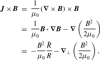 $$\begin{eqnarray}\displaystyle \boldsymbol{J}\times \boldsymbol{B} & = & \displaystyle \frac{1}{\unicode[STIX]{x1D707}_{0}}(\unicode[STIX]{x1D735}\times \boldsymbol{B})\times \boldsymbol{B}\nonumber\\ \displaystyle & = & \displaystyle \frac{1}{\unicode[STIX]{x1D707}_{0}}\boldsymbol{B}\boldsymbol{\cdot }\unicode[STIX]{x1D735}\boldsymbol{B}-\unicode[STIX]{x1D735}\left(\frac{B^{2}}{2\unicode[STIX]{x1D707}_{0}}\right)\nonumber\\ \displaystyle & = & \displaystyle -\frac{B^{2}}{\unicode[STIX]{x1D707}_{0}}\frac{\hat{R}}{R}-\unicode[STIX]{x1D735}_{\bot }\left(\frac{B^{2}}{2\unicode[STIX]{x1D707}_{0}}\right),\end{eqnarray}$$
where
 $R$
is the local radius of curvature and
$R$
is the local radius of curvature and
 $\hat{R}$
is a radial unit vector pointing from the local centre of curvature of a field line to the field line. The subscript
$\hat{R}$
is a radial unit vector pointing from the local centre of curvature of a field line to the field line. The subscript
 $\bot$
refers to the direction perpendicular to the magnetic field. The two terms in (2.57) are denoted respectively as the curvature and the gradient term. These two terms are not necessarily orthogonal and in the case of a vacuum magnetic field, the two terms are equal and opposite since
$\bot$
refers to the direction perpendicular to the magnetic field. The two terms in (2.57) are denoted respectively as the curvature and the gradient term. These two terms are not necessarily orthogonal and in the case of a vacuum magnetic field, the two terms are equal and opposite since
 $\boldsymbol{J}=0$
for a vacuum field. The magnetic force associated with the curvature term
$\boldsymbol{J}=0$
for a vacuum field. The magnetic force associated with the curvature term
 $-\unicode[STIX]{x1D707}_{0}^{-1}B^{2}\hat{R}/R$
acts to decrease or straighten out the curvature while the magnetic force associated with the gradient term
$-\unicode[STIX]{x1D707}_{0}^{-1}B^{2}\hat{R}/R$
acts to decrease or straighten out the curvature while the magnetic force associated with the gradient term
 $-\unicode[STIX]{x1D735}_{\bot }(B^{2}/2\unicode[STIX]{x1D707}_{0})$
pushes from regions of large
$-\unicode[STIX]{x1D735}_{\bot }(B^{2}/2\unicode[STIX]{x1D707}_{0})$
pushes from regions of large
 $B^{2}$
to regions of small
$B^{2}$
to regions of small
 $B^{2}$
but only in the direction perpendicular to
$B^{2}$
but only in the direction perpendicular to
 $\boldsymbol{B}$
.
$\boldsymbol{B}$
.
The jet can be subdivided into the jet main column and the jet tip as indicated in figure 1. The jet main column consists of most of the jet length
 $l$
and in the main column the jet is highly collimated with
$l$
and in the main column the jet is highly collimated with
 $B_{z}\gg B_{r}$
and
$B_{z}\gg B_{r}$
and
 $U_{z}\gg U_{r}$
. Thus, in the main column the magnetic field is nearly straight so the curvature term is small in (2.57). However, the field curvature is large in the tip region and the curvature force provides a local retardation of the jet in this region (see figure 1) which provides the stagnation and mass pile-up that causes amplification of
$U_{z}\gg U_{r}$
. Thus, in the main column the magnetic field is nearly straight so the curvature term is small in (2.57). However, the field curvature is large in the tip region and the curvature force provides a local retardation of the jet in this region (see figure 1) which provides the stagnation and mass pile-up that causes amplification of
 $B_{\unicode[STIX]{x1D719}}$
and hence collimation. The field curvature at the tip is quite evident in the 6 through
$B_{\unicode[STIX]{x1D719}}$
and hence collimation. The field curvature at the tip is quite evident in the 6 through
 $8~\unicode[STIX]{x03BC}\text{s}$
frames in figure 3.
$8~\unicode[STIX]{x03BC}\text{s}$
frames in figure 3.
The poloidal magnetic flux of a magnetic dipole located at
 $z=-h$
is given by
$z=-h$
is given by
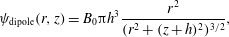 $$\begin{eqnarray}\unicode[STIX]{x1D713}_{\text{dipole}}(r,z)=B_{0}\unicode[STIX]{x03C0}h^{3}\frac{r^{2}}{(r^{2}+(z+h)^{2})^{3/2}},\end{eqnarray}$$
where
 $B_{0}$
is defined such that
$B_{0}$
is defined such that
 $\boldsymbol{B}=B_{0}\hat{z}$
at
$\boldsymbol{B}=B_{0}\hat{z}$
at
 $r=0,z=0$
. The corresponding poloidal magnetic field in the upper half-volume defined by
$r=0,z=0$
. The corresponding poloidal magnetic field in the upper half-volume defined by
 $z>0$
is given by inserting (2.58) in (2.19) and this magnetic field is a vacuum magnetic field as can be seen by inserting (2.58) in (2.23). Consideration of (2.58) in the
$z>0$
is given by inserting (2.58) in (2.19) and this magnetic field is a vacuum magnetic field as can be seen by inserting (2.58) in (2.23). Consideration of (2.58) in the
 $z=0$
plane shows that in this plane
$z=0$
plane shows that in this plane
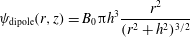 $$\begin{eqnarray}\unicode[STIX]{x1D713}_{\text{dipole}}(r,z)=B_{0}\unicode[STIX]{x03C0}h^{3}\frac{r^{2}}{(r^{2}+h^{2})^{3/2}}\end{eqnarray}$$
and so in this plane
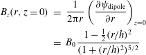 $$\begin{eqnarray}\displaystyle B_{z}(r,z=0) & = & \displaystyle \frac{1}{2\unicode[STIX]{x03C0}r}\left(\frac{\unicode[STIX]{x2202}\unicode[STIX]{x1D713}_{\text{dipole}}}{\unicode[STIX]{x2202}r}\right)_{z=0}\nonumber\\ \displaystyle & = & \displaystyle B_{0}\frac{1-{\textstyle \frac{1}{2}}(r/h)^{2}}{(1+(r/h)^{2})^{5/2}}\end{eqnarray}$$
so
 $B_{z}$
reverses polarity at
$B_{z}$
reverses polarity at
 $r=\sqrt{2}h$
. A jet poloidal magnetic field can then be considered as the stretching in the
$r=\sqrt{2}h$
. A jet poloidal magnetic field can then be considered as the stretching in the
 $z$
direction of a poloidal flux that is initially given by (2.58) while maintaining the
$z$
direction of a poloidal flux that is initially given by (2.58) while maintaining the
 $z=0$
plane boundary condition prescribed by (2.59) or equivalently by the associated (2.60).
$z=0$
plane boundary condition prescribed by (2.59) or equivalently by the associated (2.60).
This stretching can be represented by replacing
 $z$
in (2.58) by a stretched version but only for regions within the length
$z$
in (2.58) by a stretched version but only for regions within the length
 $l$
of the jet because for
$l$
of the jet because for
 $z>l$
there is no jet and the magnetic field must revert to being the dipole field. Thus, we make the replacement
$z>l$
there is no jet and the magnetic field must revert to being the dipole field. Thus, we make the replacement
 $z\rightarrow z\unicode[STIX]{x1D70E}(z)$
in (2.58) where
$z\rightarrow z\unicode[STIX]{x1D70E}(z)$
in (2.58) where
 $\unicode[STIX]{x1D70E}(z)=\unicode[STIX]{x1D700}$
for
$\unicode[STIX]{x1D70E}(z)=\unicode[STIX]{x1D700}$
for
 $0<z<l$
and then
$0<z<l$
and then
 $\unicode[STIX]{x1D70E}(z)$
abruptly becomes equal to unity as soon as
$\unicode[STIX]{x1D70E}(z)$
abruptly becomes equal to unity as soon as
 $z$
exceeds
$z$
exceeds
 $l.$
A possible functional form for
$l.$
A possible functional form for
 $\unicode[STIX]{x1D70E}$
is
$\unicode[STIX]{x1D70E}$
is
 $$\begin{eqnarray}\unicode[STIX]{x1D70E}(z)=\frac{1}{1+\unicode[STIX]{x1D700}}\left(\frac{\text{e}^{2(z-l)/h}}{1+\text{e}^{2(z-l)/h}}+\unicode[STIX]{x1D700}\right).\end{eqnarray}$$
Thus, equation (2.58) is replaced by
 $$\begin{eqnarray}\unicode[STIX]{x1D713}(r,z)=B_{0}\unicode[STIX]{x03C0}h^{3}\frac{r^{2}}{(r^{2}+(z\unicode[STIX]{x1D70E}(z)+h)^{2})^{3/2}},\end{eqnarray}$$
which reverts to (2.59) at
 $z=0$
and so satisfies the same boundary conditions as the vacuum field. It is seen that as the jet becomes very long so
$z=0$
and so satisfies the same boundary conditions as the vacuum field. It is seen that as the jet becomes very long so
 $\unicode[STIX]{x1D70E}(z)$
becomes very small, the dependence of
$\unicode[STIX]{x1D70E}(z)$
becomes very small, the dependence of
 $\unicode[STIX]{x1D713}$
on
$\unicode[STIX]{x1D713}$
on
 $z$
becomes very weak and so
$z$
becomes very weak and so
 $B_{r}$
becomes much smaller than
$B_{r}$
becomes much smaller than
 $B_{z}$
because
$B_{z}$
because
 $B_{r}/B_{z}=-(\unicode[STIX]{x2202}\unicode[STIX]{x1D713}/\unicode[STIX]{x2202}z)/(\unicode[STIX]{x2202}\unicode[STIX]{x1D713}/\unicode[STIX]{x2202}r)$
. In this
$B_{r}/B_{z}=-(\unicode[STIX]{x2202}\unicode[STIX]{x1D713}/\unicode[STIX]{x2202}z)/(\unicode[STIX]{x2202}\unicode[STIX]{x1D713}/\unicode[STIX]{x2202}r)$
. In this
 $z<l$
region and for
$z<l$
region and for
 $r\ll h$
, it is seen that
$r\ll h$
, it is seen that
 $\unicode[STIX]{x1D713}\sim r^{2}$
which justifies the form of (2.34) and also the neglect of
$\unicode[STIX]{x1D713}\sim r^{2}$
which justifies the form of (2.34) and also the neglect of
 $\unicode[STIX]{x1D735}\boldsymbol{\cdot }(r^{-2}\unicode[STIX]{x1D735}\unicode[STIX]{x1D713})$
in (2.24a
) and (2.24c
) in the jet main column.
$\unicode[STIX]{x1D735}\boldsymbol{\cdot }(r^{-2}\unicode[STIX]{x1D735}\unicode[STIX]{x1D713})$
in (2.24a
) and (2.24c
) in the jet main column.
Figure 4 shows plots of
 $\unicode[STIX]{x1D713}(r,z)$
as given by (2.62) and (2.61) for increasing values of
$\unicode[STIX]{x1D713}(r,z)$
as given by (2.62) and (2.61) for increasing values of
 $l$
. These plots show that the magnetic field lines are nearly straight in the main column and then curve around at the jet tip. There is a concentration of field lines at the jet tip where this curvature occurs and this concentration comes from the abrupt change in
$l$
. These plots show that the magnetic field lines are nearly straight in the main column and then curve around at the jet tip. There is a concentration of field lines at the jet tip where this curvature occurs and this concentration comes from the abrupt change in
 $\unicode[STIX]{x1D70E}$
which causes
$\unicode[STIX]{x1D70E}$
which causes
 $\unicode[STIX]{x1D713}$
to have a large gradient in the
$\unicode[STIX]{x1D713}$
to have a large gradient in the
 $z$
direction and thus
$z$
direction and thus
 $B_{r}$
to have a large value. Both the curvature and gradient forces point downward in regions just below the maximum value of
$B_{r}$
to have a large value. Both the curvature and gradient forces point downward in regions just below the maximum value of
 $B_{r}$
(i.e. below where flux surfaces are horizontal and have maximum density) and so give a retarding force. However, just above the maximum value of
$B_{r}$
(i.e. below where flux surfaces are horizontal and have maximum density) and so give a retarding force. However, just above the maximum value of
 $B_{r}$
the curvature force points down while the gradient force points up, so the curvature and gradient forces tend to cancel; this corresponds to the magnetic field tending to be a vacuum field in the region above the maximum value of
$B_{r}$
the curvature force points down while the gradient force points up, so the curvature and gradient forces tend to cancel; this corresponds to the magnetic field tending to be a vacuum field in the region above the maximum value of
 $B_{r}$
,
$B_{r}$
,


3 Experimental set-up
Creating a jet requires three ingredients, namely poloidal flux, poloidal current and a mass flux at the jet source and these must all be axisymmetric. The Caltech jet experiment takes place in the 1.4 m diameter, 2 m long vacuum chamber sketched in figure 2. The jet emanates from a concentric set of electrodes located at one end of the chamber. As stated in the Introduction the electrodes consist of a 20 cm diameter copper disk surrounded by a coplanar 50 cm diameter copper annulus with a 6 mm gap between the disk and the annulus so that the disk and annulus can be at different electrostatic potentials. A coil coaxial with the disk and annulus and located just behind the gap generates a dipole-like poloidal magnetic field that links the disk to the annulus. The coil current lasts approximately 5 ms which greatly exceeds all other experimental time scales and so can be considered as being effectively steady state. Because the copper disk and annulus act like perfect conductors on the
 ${<}50~\unicode[STIX]{x03BC}\text{s}$
time scale of the jet experiment, but as resistive conductors on the 5 ms time scale of the coil current, the magnetic flux produced by the coil diffuses into the copper disk and annulus when the coil is turned on, but then is frozen into the disk and annulus on the
${<}50~\unicode[STIX]{x03BC}\text{s}$
time scale of the jet experiment, but as resistive conductors on the 5 ms time scale of the coil current, the magnetic flux produced by the coil diffuses into the copper disk and annulus when the coil is turned on, but then is frozen into the disk and annulus on the
 ${<}50~\unicode[STIX]{x03BC}\text{s}$
time scale of the jet experiment. The plane of disk and annulus defines the
${<}50~\unicode[STIX]{x03BC}\text{s}$
time scale of the jet experiment. The plane of disk and annulus defines the
 $z=0$
plane and so poloidal flux is fixed in the
$z=0$
plane and so poloidal flux is fixed in the
 $z=0$
plane consistent with (2.62). The total poloidal flux has been measured using flux loops that integrate the voltage induced in a loop and these measurements show that the poloidal flux is 0.5–2 mWb. Each of the disk and annulus have eight holes through which neutral gas is puffed by fast electrically pulsed valves. The neutral gas density is large near the holes but falls off rapidly in a few centimetres. Various gas species are used with hydrogen, argon and nitrogen being used most frequently. The gas valves have plenums that release a fixed amount of gas into approximately 1 m long copper tubes that go to holes on the electrodes from which the gas is ejected into the vacuum chamber. The gas valve timing is quite critical and is adjusted so that the peak gas pressure at
$z=0$
plane consistent with (2.62). The total poloidal flux has been measured using flux loops that integrate the voltage induced in a loop and these measurements show that the poloidal flux is 0.5–2 mWb. Each of the disk and annulus have eight holes through which neutral gas is puffed by fast electrically pulsed valves. The neutral gas density is large near the holes but falls off rapidly in a few centimetres. Various gas species are used with hydrogen, argon and nitrogen being used most frequently. The gas valves have plenums that release a fixed amount of gas into approximately 1 m long copper tubes that go to holes on the electrodes from which the gas is ejected into the vacuum chamber. The gas valve timing is quite critical and is adjusted so that the peak gas pressure at
 $z=0$
coincides with the time of plasma breakdown. If the peak gas pressure occurs much before breakdown, there will be substantial neutral gas in the vacuum chamber and the jet will interact with this gas. Having peak gas pressure long after breakdown is less serious, but means that the cryopump which evacuates the chamber will fill up with gas more quickly and so will have to be purged more often. The gas valve timing has to take into account the time for the gas to travel from the valve to the electrodes; this delay is inversely proportional to the gas thermal velocity and so is greater for the heavier gases. Typical delay times are of the order of one to a few ms depending on the gas species.
$z=0$
coincides with the time of plasma breakdown. If the peak gas pressure occurs much before breakdown, there will be substantial neutral gas in the vacuum chamber and the jet will interact with this gas. Having peak gas pressure long after breakdown is less serious, but means that the cryopump which evacuates the chamber will fill up with gas more quickly and so will have to be purged more often. The gas valve timing has to take into account the time for the gas to travel from the valve to the electrodes; this delay is inversely proportional to the gas thermal velocity and so is greater for the heavier gases. Typical delay times are of the order of one to a few ms depending on the gas species.
The gas valve timing and pressure are arranged so that the neutral gas in the region between the disk and annulus satisfies the Paschen breakdown condition. The Paschen criterion for hydrogen indicates that the minimum voltage required for breakdown occurs when the product of neutral gas pressure and the distance between electrodes is approximately 2 torr cm. The voltage for breakdown at this minimum is 300 V. In actual practice, the applied voltage is 2–6 kV and the effective distance between electrodes is a few tens of cm. Supplying gas at the eight annulus holes is essential to have breakdown, but once the plasma has broken down, the gas coming from the annulus holes has little influence. On the other hand, after breakdown the gas supplied from the eight disk holes becomes the source of plasma for the jet and the density of this gas affects the density of the plasma in the jet. The vacuum chamber is typically evacuated before firing a shot so there is no pre-existing gas outside the jet. However, as discussed in § 9 it is also possible to arrange for the vacuum chamber to contain a target cloud of pre-existing gas which the jet impacts and stagnates against. At the present time, experiments have not been done with a uniform surrounding background gas. However, the vacuum chamber walls act in a sense like a cocoon of surrounding background gas because the walls act as a flux conserver. A cocoon of surrounding conducting background gas would also be a flux conserver to the extent that the jet magnetic field cannot penetrate the cocoon.
Two different power supplies have been used to provide the breakdown voltage and power the jet; these power supplies can be used separately or together. The first and original power supply consists of a pair of
 $59~\unicode[STIX]{x03BC}\text{F}$
high-energy capacitors connected in parallel. These capacitors are charged to 2–6 kV and then electronically switched via Type A ignitrons to four low-inductance coaxial cables that go to the electrodes. The electrical design is optimized to minimize inductance in order to drive maximum electric current. This power supply provides a sine wave current having a rise time of about
$59~\unicode[STIX]{x03BC}\text{F}$
high-energy capacitors connected in parallel. These capacitors are charged to 2–6 kV and then electronically switched via Type A ignitrons to four low-inductance coaxial cables that go to the electrodes. The electrical design is optimized to minimize inductance in order to drive maximum electric current. This power supply provides a sine wave current having a rise time of about
 $5{-}7~\unicode[STIX]{x03BC}\text{s}$
(Kumar, Moser & Bellan Reference Kumar, Moser and Bellan2010). The second and newer power supply is a pulse forming network (PFN) consisting of ten
$5{-}7~\unicode[STIX]{x03BC}\text{s}$
(Kumar, Moser & Bellan Reference Kumar, Moser and Bellan2010). The second and newer power supply is a pulse forming network (PFN) consisting of ten
 $120~\unicode[STIX]{x03BC}\text{F}$
capacitors connected as five pairs of capacitors with a small inductance between each pair (Moser Reference Moser2012). The capacitance and inductance were chosen so that the PFN provides a flat-top current lasting
$120~\unicode[STIX]{x03BC}\text{F}$
capacitors connected as five pairs of capacitors with a small inductance between each pair (Moser Reference Moser2012). The capacitance and inductance were chosen so that the PFN provides a flat-top current lasting
 $50~\unicode[STIX]{x03BC}\text{s}$
. The PFN was designed to match the nominal jet impedance. Typically, the first power supply creates the jet and the PFN sustains the jet. From an electrical point of view, before breakdown the load looks like an open circuit (infinite impedance) and after breakdown like a nearly short circuit (low impedance). The behaviour after breakdown is such that the power supply behaves like a current source driving a nominal
$50~\unicode[STIX]{x03BC}\text{s}$
. The PFN was designed to match the nominal jet impedance. Typically, the first power supply creates the jet and the PFN sustains the jet. From an electrical point of view, before breakdown the load looks like an open circuit (infinite impedance) and after breakdown like a nearly short circuit (low impedance). The behaviour after breakdown is such that the power supply behaves like a current source driving a nominal
 $20~\text{m}\unicode[STIX]{x03A9}$
load; specifically the nominal load current is 100 kA and the nominal load voltage is 2 kV. The PFN was designed to match this
$20~\text{m}\unicode[STIX]{x03A9}$
load; specifically the nominal load current is 100 kA and the nominal load voltage is 2 kV. The PFN was designed to match this
 $20~\text{m}\unicode[STIX]{x03A9}$
impedance. The effect of using the PFN in addition to the original capacitor pair is to make the current waveform last longer in which case the jet lasts longer and so attains greater length.
$20~\text{m}\unicode[STIX]{x03A9}$
impedance. The effect of using the PFN in addition to the original capacitor pair is to make the current waveform last longer in which case the jet lasts longer and so attains greater length.
The magnetic field and plasma density have substantial spatial variation but peak axial magnetic fields are from 0.1 to 0.6 T near the electrodes, peak currents are approximately 100 kA and peak densities are
 $n=10^{22}{-}10^{23}~\text{m}^{-3}$
. The temperature is much less variable and is typically 2–4 eV. Shikama & Bellan (Reference Shikama and Bellan2013) made detailed spectroscopic measurements near the electrodes in a nitrogen plasma. These measurements indicated a peak density of
$n=10^{22}{-}10^{23}~\text{m}^{-3}$
. The temperature is much less variable and is typically 2–4 eV. Shikama & Bellan (Reference Shikama and Bellan2013) made detailed spectroscopic measurements near the electrodes in a nitrogen plasma. These measurements indicated a peak density of
 $n=10^{23}~\text{m}^{-3}$
using Stark broadening and a peak magnetic field
$n=10^{23}~\text{m}^{-3}$
using Stark broadening and a peak magnetic field
 $B=0.6~\text{T}$
using Zeeman splitting. These give an Alfvén velocity
$B=0.6~\text{T}$
using Zeeman splitting. These give an Alfvén velocity
 $v_{A}=10~\text{km}~\text{s}^{-1}$
and a plasma
$v_{A}=10~\text{km}~\text{s}^{-1}$
and a plasma
 $\unicode[STIX]{x1D6FD}=0.1$
near the electrodes. The jet radius is approximately 2 cm at this location.
$\unicode[STIX]{x1D6FD}=0.1$
near the electrodes. The jet radius is approximately 2 cm at this location.
Because of the large density and low temperature, the mean free path is very small compared to the system size and is of the order of microns. Nevertheless, as discussed in § 7 there are circumstances where two-fluid and kinetic effects become apparent because of large local stresses.
Figure 3 from You et al. (Reference You, Yun and Bellan2005) shows the formation, propagation and kink destabilization of a jet created using the original power supply, i.e. no PFN is used. This figure shows that initially (
 $4~\unicode[STIX]{x03BC}\text{s}$
) there are eight plasma-filled flux tubes spanning from a hole on the disk to a hole on the annulus; these are called the spider legs because of their appearance. As time progresses, the inner spider legs merge at about
$4~\unicode[STIX]{x03BC}\text{s}$
) there are eight plasma-filled flux tubes spanning from a hole on the disk to a hole on the annulus; these are called the spider legs because of their appearance. As time progresses, the inner spider legs merge at about
 $7~\unicode[STIX]{x03BC}\text{s}$
to form the jet main column which then continuously increases in length (
$7~\unicode[STIX]{x03BC}\text{s}$
to form the jet main column which then continuously increases in length (
 $7{-}10~\unicode[STIX]{x03BC}\text{s}$
) until a kink instability develops. The diameter of the circle (disk electrode) in figure 3 is 20 cm.
$7{-}10~\unicode[STIX]{x03BC}\text{s}$
) until a kink instability develops. The diameter of the circle (disk electrode) in figure 3 is 20 cm.
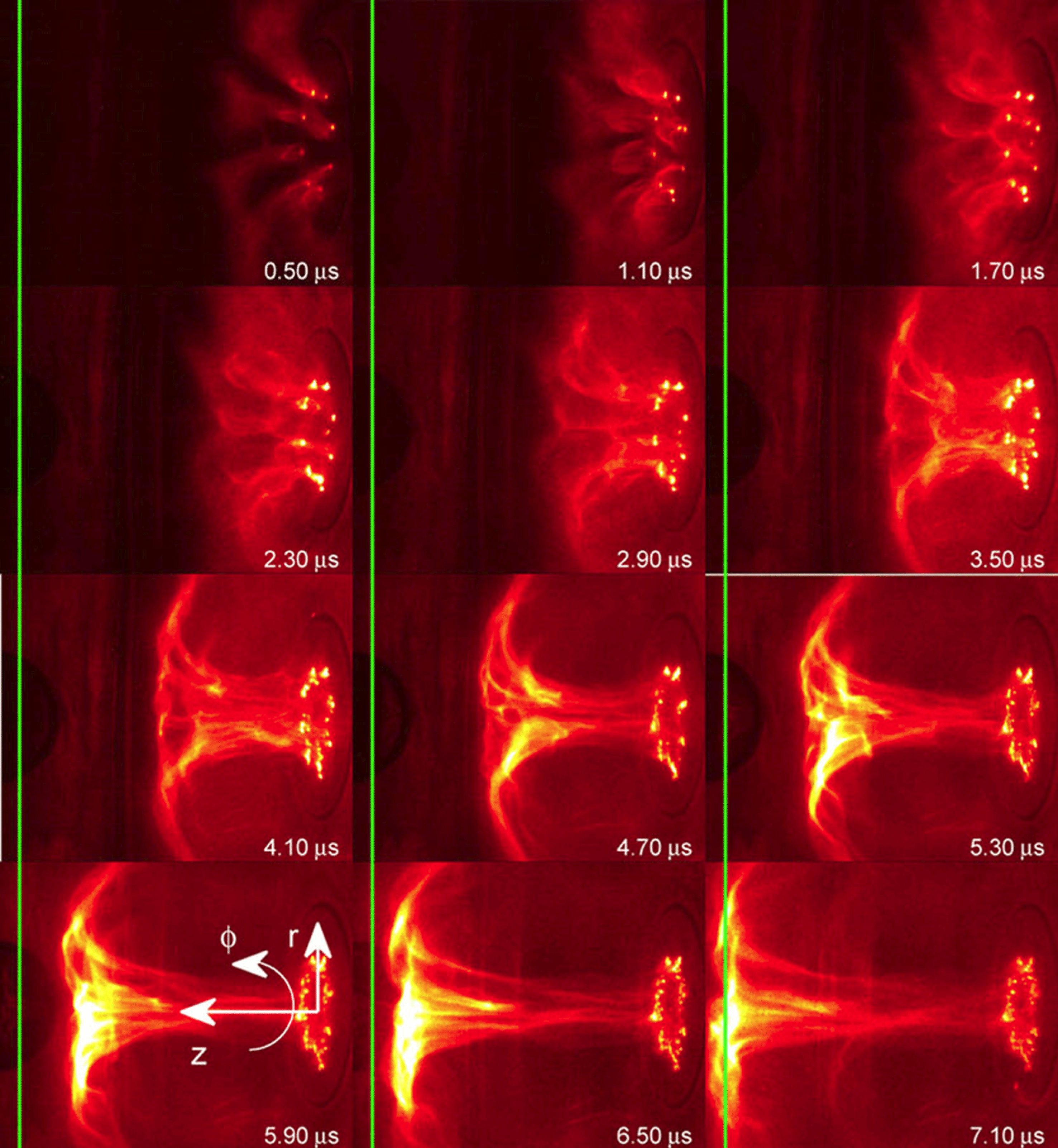
Figure 5. Green line shows interferometer laser beam location. [Reprinted figure with permission from Kumar and Bellan, Physical Review Letters 103, 105003 (2009). Copyright 2009 by the American Physical Society.]
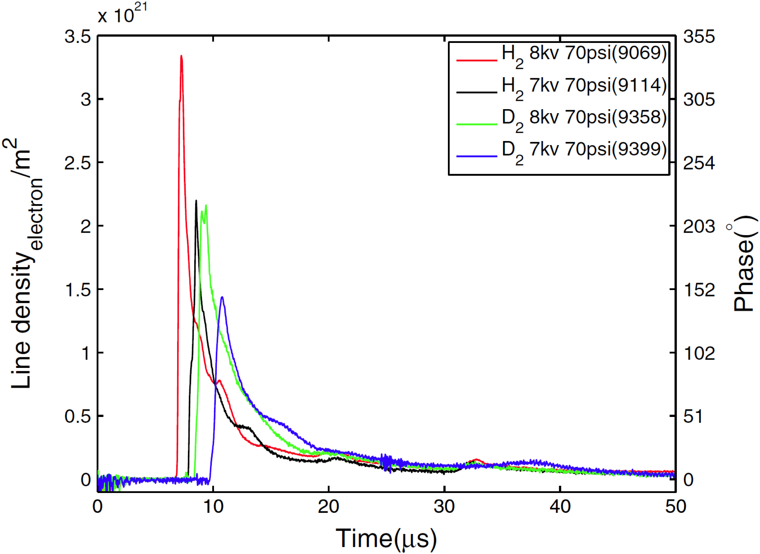
Figure 6. Time dependence of interferometer signal for hydrogen and deuterium plasma jets at two different capacitor bank settings. The jet velocity is faster (i.e. front appears earlier) for hydrogen than for deuterium (compare red to green and black to blue) and is faster for a higher voltage setting (compare red to black and green to blue). [Reprinted figure with permission from Kumar and Bellan, Physical Review Letters 103, 105003 (2009). Copyright 2009 by the American Physical Society.]
4 Jet flow velocity, collimation and tip stagnation
The jet flow velocity has been measured by Kumar & Bellan (Reference Kumar and Bellan2009) using a laser interferometer. The laser beam, shown as a green line in figure 5, propagated at right angles to the jet motion so that the density measured by the interferometer has a time dependence such that the initial rise time of the interferometer signal corresponded to the tip of the jet intercepting the laser beam. In the figure the jet tip passes the laser beam at approximately
 $7~\unicode[STIX]{x03BC}\text{s}$
. The time profile of the interferometer signal would then very roughly correspond to the axial dependence of the line-averaged density; this is seen in figure 6. The interferometer signal exploits the plasma wave dispersion relation
$7~\unicode[STIX]{x03BC}\text{s}$
. The time profile of the interferometer signal would then very roughly correspond to the axial dependence of the line-averaged density; this is seen in figure 6. The interferometer signal exploits the plasma wave dispersion relation
 $\unicode[STIX]{x1D714}^{2}=\unicode[STIX]{x1D714}_{pe}^{2}+k^{2}c^{2}$
so
$\unicode[STIX]{x1D714}^{2}=\unicode[STIX]{x1D714}_{pe}^{2}+k^{2}c^{2}$
so
 $k=\sqrt{\unicode[STIX]{x1D714}^{2}-\unicode[STIX]{x1D714}_{pe}^{2}}/c$
. The phase
$k=\sqrt{\unicode[STIX]{x1D714}^{2}-\unicode[STIX]{x1D714}_{pe}^{2}}/c$
. The phase
 $\unicode[STIX]{x1D711}$
of the interferometer leg through the plasma is given by
$\unicode[STIX]{x1D711}$
of the interferometer leg through the plasma is given by
 $$\begin{eqnarray}\unicode[STIX]{x1D711}=\int \,\text{d}y\,k=\frac{\unicode[STIX]{x1D714}}{c}\int \,\text{d}y\sqrt{1-\frac{\unicode[STIX]{x1D714}_{pe}^{2}(y)}{\unicode[STIX]{x1D714}^{2}}}.\end{eqnarray}$$
Since the laser frequency
 $\unicode[STIX]{x1D714}$
greatly exceeds the plasma frequency
$\unicode[STIX]{x1D714}$
greatly exceeds the plasma frequency
 $\unicode[STIX]{x1D714}_{pe}$
, the phase can be written as
$\unicode[STIX]{x1D714}_{pe}$
, the phase can be written as
 $$\begin{eqnarray}\unicode[STIX]{x1D711}\simeq \frac{\unicode[STIX]{x1D714}}{c}\int \,\text{d}y\left(1-\frac{\unicode[STIX]{x1D714}_{pe}^{2}(y)}{2\unicode[STIX]{x1D714}^{2}}\right)\end{eqnarray}$$
and so the change in phase that occurs when plasma passes through the laser beam is
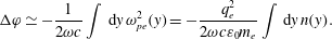 $$\begin{eqnarray}\unicode[STIX]{x0394}\unicode[STIX]{x1D711}\simeq -\frac{1}{2\unicode[STIX]{x1D714}c}\int \,\text{d}y\,\unicode[STIX]{x1D714}_{pe}^{2}(y)=-\frac{q_{e}^{2}}{2\unicode[STIX]{x1D714}c\unicode[STIX]{x1D700}_{0}m_{e}}\int \,\text{d}y\,n(y).\end{eqnarray}$$
Thus, the interferometer phase shift
 $\unicode[STIX]{x0394}\unicode[STIX]{x1D711}$
that occurs when the plasma traverses the laser beam is proportional to the line-averaged density. The laser beam is 29 cm from the electrode plane and so the jet velocity is defined as this distance divided by the time at which the jet front passes the interferometer beam (green line in figure 5). Thus, the jet velocity in figure 5 would be
$\unicode[STIX]{x0394}\unicode[STIX]{x1D711}$
that occurs when the plasma traverses the laser beam is proportional to the line-averaged density. The laser beam is 29 cm from the electrode plane and so the jet velocity is defined as this distance divided by the time at which the jet front passes the interferometer beam (green line in figure 5). Thus, the jet velocity in figure 5 would be
 $0.29~\text{m}/7~\unicode[STIX]{x03BC}\text{s}=41~\text{km}~\text{s}^{-1}$
. By charging the capacitor bank to different voltages and measuring the resultant electric current flowing in the jet and the jet velocity, a plot of jet velocity versus current can be made. This was done separately for hydrogen and for deuterium plasma jets and a plot of velocity versus current is shown in figure 7. This plot shows that hydrogen is faster than deuterium by approximately the square root of the mass ratio consistent with the scaling in (2.40). The straight lines in figure 7 go approximately through the origin confirming that velocity is linearly proportional to current.
$0.29~\text{m}/7~\unicode[STIX]{x03BC}\text{s}=41~\text{km}~\text{s}^{-1}$
. By charging the capacitor bank to different voltages and measuring the resultant electric current flowing in the jet and the jet velocity, a plot of jet velocity versus current can be made. This was done separately for hydrogen and for deuterium plasma jets and a plot of velocity versus current is shown in figure 7. This plot shows that hydrogen is faster than deuterium by approximately the square root of the mass ratio consistent with the scaling in (2.40). The straight lines in figure 7 go approximately through the origin confirming that velocity is linearly proportional to current.
The high initial density at early times in figure 6 is consistent with the argument in §§ 2.7 and 2.9 that the jet main column stagnates against the jet tip, much like a stream of fast cars on a highway slows down and bunches up when it reaches a group of slow moving cars.
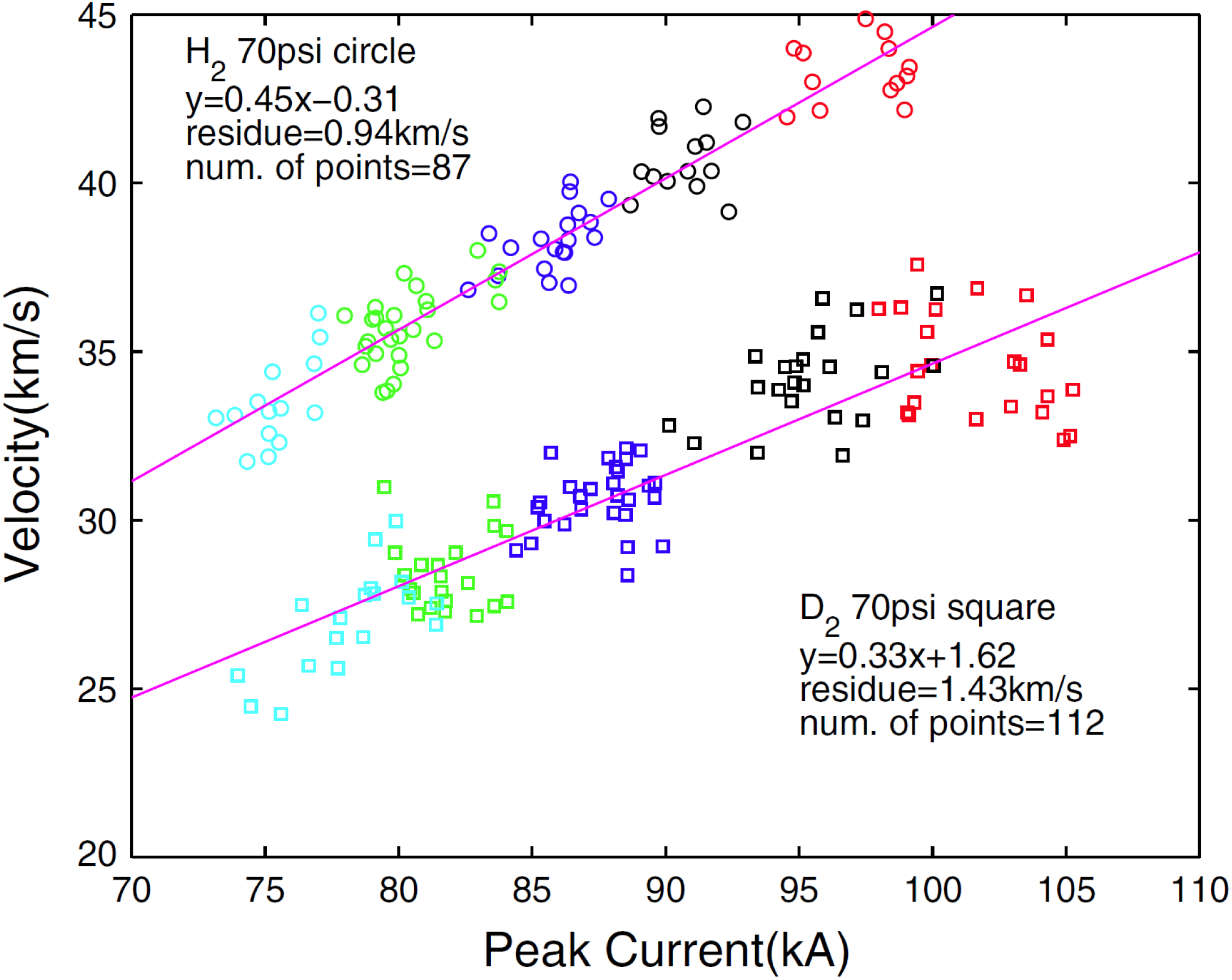
Figure 7. Velocity measured using laser interferometer versus peak electric current flowing through the plasma. The different colours are different capacitor charge voltages. [Reprinted figure with permission from Kumar and Bellan, Physical Review Letters 103, 105003 (2009). Copyright 2009 by the American Physical Society.]
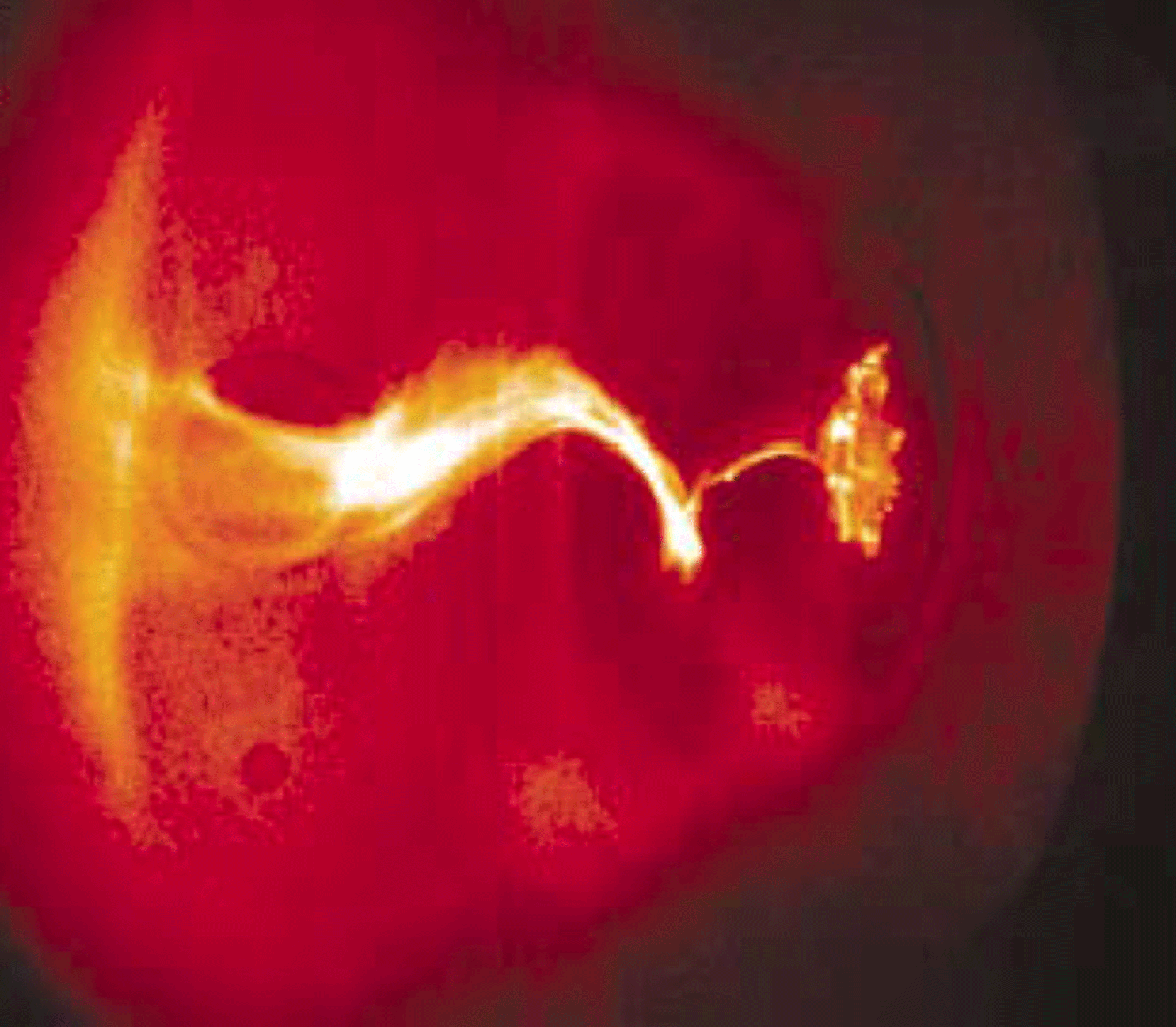
Figure 8. Photo of a kink instability extracted from figure 3 of Hsu and Bellan. [Reprinted figure with permission from Hsu and Bellan, Physical Review Letters 90, 215002 (2003). Copyright 2003 by the American Physical Society.]
The axial dependence of axial velocity and associated density has been measured by Yun & Bellan (Reference Yun and Bellan2010) using Stark broadening of atomic lines to determine density and using Doppler shift to determine velocity. These measurements show a large increase in density near the jet tip associated with reduction of axial velocity near the jet tip, i.e. a stagnation of the jet near the tip consistent with the collimation mechanism discussed in § 2.7. These measurements also show that the density of the plasma in the main column is not the result of ionizing pre-existing neutral gas but rather comes from the injection of plasma coming from the mass source at the inner electrode. This is because the density in the jet main column is much higher than the density of any pre-existing neutral gas even if pinching of plasma formed by this pre-existing gas is taken into account.
5 Kink instability
A plasma having toroidal magnetic field only (i.e. a
 $Z$
-pinch) is subject to an axisymmetric instability called the sausage or necking instability. This instability involves conversion of stored magnetic energy into bulk kinetic energy in a manner analogous to the conversion of potential energy into kinetic energy when a ball rolls down a hill. Addition of a poloidal field stabilizes the sausage because an axisymmetric compression of a poloidal field increases the stored magnetic energy (this increase will be discussed further in § 10). However, the presence of both a poloidal magnetic field and a toroidal magnetic field makes the plasma subject to a non-axisymmetric instability called the kink instability. The sausage instability has
$Z$
-pinch) is subject to an axisymmetric instability called the sausage or necking instability. This instability involves conversion of stored magnetic energy into bulk kinetic energy in a manner analogous to the conversion of potential energy into kinetic energy when a ball rolls down a hill. Addition of a poloidal field stabilizes the sausage because an axisymmetric compression of a poloidal field increases the stored magnetic energy (this increase will be discussed further in § 10). However, the presence of both a poloidal magnetic field and a toroidal magnetic field makes the plasma subject to a non-axisymmetric instability called the kink instability. The sausage instability has
 $m=0$
symmetry whereas the kink has
$m=0$
symmetry whereas the kink has
 $m=1$
symmetry. A plot of the threshold for sausage and kink instabilities in a plasma having both poloidal and toroidal magnetic fields shows that the kink is destabilized before the sausage; see von der Linden & You (Reference von der Linden and You2017).
$m=1$
symmetry. A plot of the threshold for sausage and kink instabilities in a plasma having both poloidal and toroidal magnetic fields shows that the kink is destabilized before the sausage; see von der Linden & You (Reference von der Linden and You2017).
An example of a kink instability is shown in figure 8 from Hsu & Bellan (Reference Hsu and Bellan2003). The kink instability can also be understood as a means by which the plasma reduces, in a flux-conserving way, the energy stored in the magnetic field. Just as in the sausage instability, the energy removed from the magnetic field goes into plasma kinetic energy so the system can be thought of as being analogous to a ball rolling off the top of a hill. The magnetic energy is the same as the inductive energy and since inductance
 $L$
is defined as the magnetic flux
$L$
is defined as the magnetic flux
 $\unicode[STIX]{x1D6F7}$
per electric current
$\unicode[STIX]{x1D6F7}$
per electric current
 $I$
, the magnetic energy can be expressed as
$I$
, the magnetic energy can be expressed as
 $$\begin{eqnarray}W=\int \frac{B^{2}}{2\unicode[STIX]{x1D707}_{0}}\,\text{d}^{3}r=\frac{LI^{2}}{2}=\frac{(LI)^{2}}{2L}=\frac{\unicode[STIX]{x1D6F7}^{2}}{2L}.\end{eqnarray}$$
A coil has more inductance than a straight wire and since flux conservation together with (5.1) imply
 $W\sim 1/L$
, the kink reduces the magnetic energy by winding the initially straight current channel to be in the form of a helix, i.e. a coil. This winding into a helix is subject to azimuthal and axial boundary conditions. The azimuthal boundary condition is that the displacement be periodic in the azimuthal direction so as to be single valued. The axial boundary condition is that the ends of the jet are tied down like the ends of a violin string. Thus, the kink is an exponentially growing perturbation with a spatial dependence
$W\sim 1/L$
, the kink reduces the magnetic energy by winding the initially straight current channel to be in the form of a helix, i.e. a coil. This winding into a helix is subject to azimuthal and axial boundary conditions. The azimuthal boundary condition is that the displacement be periodic in the azimuthal direction so as to be single valued. The axial boundary condition is that the ends of the jet are tied down like the ends of a violin string. Thus, the kink is an exponentially growing perturbation with a spatial dependence
 $\exp (\text{i}\boldsymbol{k}\boldsymbol{\cdot }\boldsymbol{x})=\exp (\text{i}m\unicode[STIX]{x1D719}+\text{i}kz)$
where
$\exp (\text{i}\boldsymbol{k}\boldsymbol{\cdot }\boldsymbol{x})=\exp (\text{i}m\unicode[STIX]{x1D719}+\text{i}kz)$
where
 $m$
is an integer and
$m$
is an integer and
 $kl/2\unicode[STIX]{x03C0}$
is an integer or half-integer. The most unstable kink mode has
$kl/2\unicode[STIX]{x03C0}$
is an integer or half-integer. The most unstable kink mode has
 $|m|=1$
and the smallest non-trivial value for
$|m|=1$
and the smallest non-trivial value for
 $k$
corresponds to the jet length being one wavelength, i.e.
$k$
corresponds to the jet length being one wavelength, i.e.
 $k=2\unicode[STIX]{x03C0}/l$
.
$k=2\unicode[STIX]{x03C0}/l$
.
The kink wavevector is oriented perpendicular to the unperturbed magnetic field since orientation parallel to the unperturbed magnetic field would require work to be done on this field and so would diminish the amount of magnetic energy available to drive the instability. Thus, the kink has
 $\boldsymbol{k}\boldsymbol{\cdot }\boldsymbol{B}_{0}=0$
where
$\boldsymbol{k}\boldsymbol{\cdot }\boldsymbol{B}_{0}=0$
where
 $\boldsymbol{B}_{0}$
is the unperturbed magnetic field and so
$\boldsymbol{B}_{0}$
is the unperturbed magnetic field and so
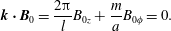 $$\begin{eqnarray}\boldsymbol{k}\boldsymbol{\cdot }\boldsymbol{B}_{0}=\frac{2\unicode[STIX]{x03C0}}{l}B_{0z}+\frac{m}{a}B_{0\unicode[STIX]{x1D719}}=0.\end{eqnarray}$$
If
 $B_{0z}$
and
$B_{0z}$
and
 $B_{0\unicode[STIX]{x1D719}}$
are positive,
$B_{0\unicode[STIX]{x1D719}}$
are positive,
 $m$
must be negative and detailed kink stability analysis shows that the most unstable mode has
$m$
must be negative and detailed kink stability analysis shows that the most unstable mode has
 $|m|=1$
and the longest possible
$|m|=1$
and the longest possible
 $l$
. The theory of tokamak kink stability defines the so-called ‘safety factor’ as
$l$
. The theory of tokamak kink stability defines the so-called ‘safety factor’ as
 $$\begin{eqnarray}q=\frac{2\unicode[STIX]{x03C0}a}{l}\frac{B_{0z}}{B_{0\unicode[STIX]{x1D719}}}\end{eqnarray}$$
so
 $m=-1$
and
$m=-1$
and
 $q=1$
correspond to satisfying the conditions for kink instability. In a tokamak the meanings of toroidal and poloidal are reversed from the meanings in the jet, i.e. the toroidal field in the jet corresponds to the poloidal field in a tokamak and vice versa. In a tokamak
$q=1$
correspond to satisfying the conditions for kink instability. In a tokamak the meanings of toroidal and poloidal are reversed from the meanings in the jet, i.e. the toroidal field in the jet corresponds to the poloidal field in a tokamak and vice versa. In a tokamak
 $a,l$
and
$a,l$
and
 $B_{0z}$
are typically fixed and so kink instability comes from having excessive
$B_{0z}$
are typically fixed and so kink instability comes from having excessive
 $B_{0\unicode[STIX]{x1D719}}$
whereas in the jet
$B_{0\unicode[STIX]{x1D719}}$
whereas in the jet
 $a$
,
$a$
,
 $B_{0\unicode[STIX]{x1D719}}$
and
$B_{0\unicode[STIX]{x1D719}}$
and
 $B_{0z}$
are typically fixed while
$B_{0z}$
are typically fixed while
 $l$
increases as the jet lengthens.
$l$
increases as the jet lengthens.
Hsu & Bellan (Reference Hsu and Bellan2003) observed the onset of the kink instability and showed via probe measurements of the internal poloidal and toroidal magnetic fields for a large range of parameters that this onset was consistent with
 $q$
dropping from an initial value exceeding unity when
$q$
dropping from an initial value exceeding unity when
 $l$
was small (i.e. jet was short) to
$l$
was small (i.e. jet was short) to
 $l$
reaching a critical value at which
$l$
reaching a critical value at which
 $q=1$
. This condition is known as the Kruskal–Shafranov kink stability condition (Shafranov Reference Shafranov1956; Kruskal & Tuck Reference Kruskal and Tuck1958) and this
$q=1$
. This condition is known as the Kruskal–Shafranov kink stability condition (Shafranov Reference Shafranov1956; Kruskal & Tuck Reference Kruskal and Tuck1958) and this
 $q=1$
condition was observed to hold for various values of
$q=1$
condition was observed to hold for various values of
 $B_{0z}$
and
$B_{0z}$
and
 $B_{0\unicode[STIX]{x1D719}}$
. The onset of kinking is evident in the
$B_{0\unicode[STIX]{x1D719}}$
. The onset of kinking is evident in the
 $11~\unicode[STIX]{x03BC}\text{s}$
frame of figure 3.
$11~\unicode[STIX]{x03BC}\text{s}$
frame of figure 3.
6 Rayleigh–Taylor instability
The kink instability is an exponentially growing helical instability so each segment of the jet makes an exponentially growing lateral displacement from its original position. This means that an observer located in the jet frame would experience an effective gravity because the exponentially growing displacement implies an exponentially growing velocity, i.e. an acceleration. The kink can be considered as a destabilized close cousin of an Alfvén wave and so the characteristic kink growth time is of the order of an Alfvén time where an Alfvén time is the transit time for an Alfvén wave. Since the jet velocity is slower than the Alfvén velocity, the kink time scale is much faster than the jet time scale and so jet motion can be neglected on the kink time scale. The effective gravity points in the direction opposite to the acceleration and so points towards the original axis of the jet. Because the plasma density in the jet is greater than outside as a result of the confining properties of the pinch force associated with the axial electric current flowing along the jet, the situation in the accelerating jet frame is that of a heavy fluid (the jet main column) on top of a light fluid (the region immediately exterior to the jet main column). The words heavy, light and ‘on top of’ are consistent with the presence of the effective gravitational field resulting from the lateral acceleration.
The situation of a heavy fluid on top of a light fluid is unstable and a rippling perturbation will excite a Rayleigh–Taylor instability (RTI) where at each ripple there is a downward motion of heavy fluid and an accompanying upward motion of light fluid so that the gravitational potential energy of the system decreases and becomes converted into the kinetic energy of the motion of the fluid in the ripples. When there is no magnetic field the RTI growth rate
 $\unicode[STIX]{x1D6FE}$
is given by
$\unicode[STIX]{x1D6FE}$
is given by
 $\unicode[STIX]{x1D6FE}^{2}=|\boldsymbol{k}_{RT}|g$
where
$\unicode[STIX]{x1D6FE}^{2}=|\boldsymbol{k}_{RT}|g$
where
 $|\boldsymbol{k}_{RT}|$
is the ripple wavevector and
$|\boldsymbol{k}_{RT}|$
is the ripple wavevector and
 $g$
is the effective gravity. However, when there is a magnetic field the growth rate changes to
$g$
is the effective gravity. However, when there is a magnetic field the growth rate changes to
 $\unicode[STIX]{x1D6FE}^{2}=|\boldsymbol{k}_{RT}|g-(\boldsymbol{k}_{RT}\boldsymbol{\cdot }\boldsymbol{B})^{2}/\unicode[STIX]{x1D707}_{0}\unicode[STIX]{x1D70C}$
where the extra term results from the work done on the equilibrium magnetic field by the perturbation (Kruskal & Schwarzschild Reference Kruskal and Schwarzschild1954). This means that the most unstable mode has
$\unicode[STIX]{x1D6FE}^{2}=|\boldsymbol{k}_{RT}|g-(\boldsymbol{k}_{RT}\boldsymbol{\cdot }\boldsymbol{B})^{2}/\unicode[STIX]{x1D707}_{0}\unicode[STIX]{x1D70C}$
where the extra term results from the work done on the equilibrium magnetic field by the perturbation (Kruskal & Schwarzschild Reference Kruskal and Schwarzschild1954). This means that the most unstable mode has
 $\boldsymbol{k}_{RT}\boldsymbol{\cdot }\boldsymbol{B}=0$
and a growth rate identical to the unmagnetized situation.
$\boldsymbol{k}_{RT}\boldsymbol{\cdot }\boldsymbol{B}=0$
and a growth rate identical to the unmagnetized situation.
Moser & Bellan (Reference Moser and Bellan2012a
) reported clear evidence of a kink-instigated RTI and measured a growth rate that was in reasonable agreement with
 $\unicode[STIX]{x1D6FE}^{2}=|\boldsymbol{k}_{RT}|g$
where
$\unicode[STIX]{x1D6FE}^{2}=|\boldsymbol{k}_{RT}|g$
where
 $|\boldsymbol{k}_{RT}|$
was determined from the ripple wavelength observed in photos,
$|\boldsymbol{k}_{RT}|$
was determined from the ripple wavelength observed in photos,
 $g$
was measured from the second derivative of the lateral displacement of the kinking jet and
$g$
was measured from the second derivative of the lateral displacement of the kinking jet and
 $\unicode[STIX]{x1D6FE}$
was measured from the time required for the RTI ripple amplitude to increase by a factor
$\unicode[STIX]{x1D6FE}$
was measured from the time required for the RTI ripple amplitude to increase by a factor
 $e$
. Figure 9 from Moser & Bellan (Reference Moser and Bellan2012a
) shows the jet developing a kink during the time
$e$
. Figure 9 from Moser & Bellan (Reference Moser and Bellan2012a
) shows the jet developing a kink during the time
 $20{-}23~\unicode[STIX]{x03BC}\text{s}$
and then the onset of a RTI at
$20{-}23~\unicode[STIX]{x03BC}\text{s}$
and then the onset of a RTI at
 $24~\unicode[STIX]{x03BC}\text{s}$
. The RTI ripples are much shorter than the kink wavelength and the RTI grows much faster than the kink. Thus, just as the jet motion can be ignored on the time scale of the kink instability, the kink dynamics can be ignored on the time scale of the RTI. In each of the kink instability and the RTI the slower dynamics (jet for the kink and kink for the RTI) provides the appropriate environment for the instability but otherwise the slow dynamics can be ignored.
$24~\unicode[STIX]{x03BC}\text{s}$
. The RTI ripples are much shorter than the kink wavelength and the RTI grows much faster than the kink. Thus, just as the jet motion can be ignored on the time scale of the kink instability, the kink dynamics can be ignored on the time scale of the RTI. In each of the kink instability and the RTI the slower dynamics (jet for the kink and kink for the RTI) provides the appropriate environment for the instability but otherwise the slow dynamics can be ignored.
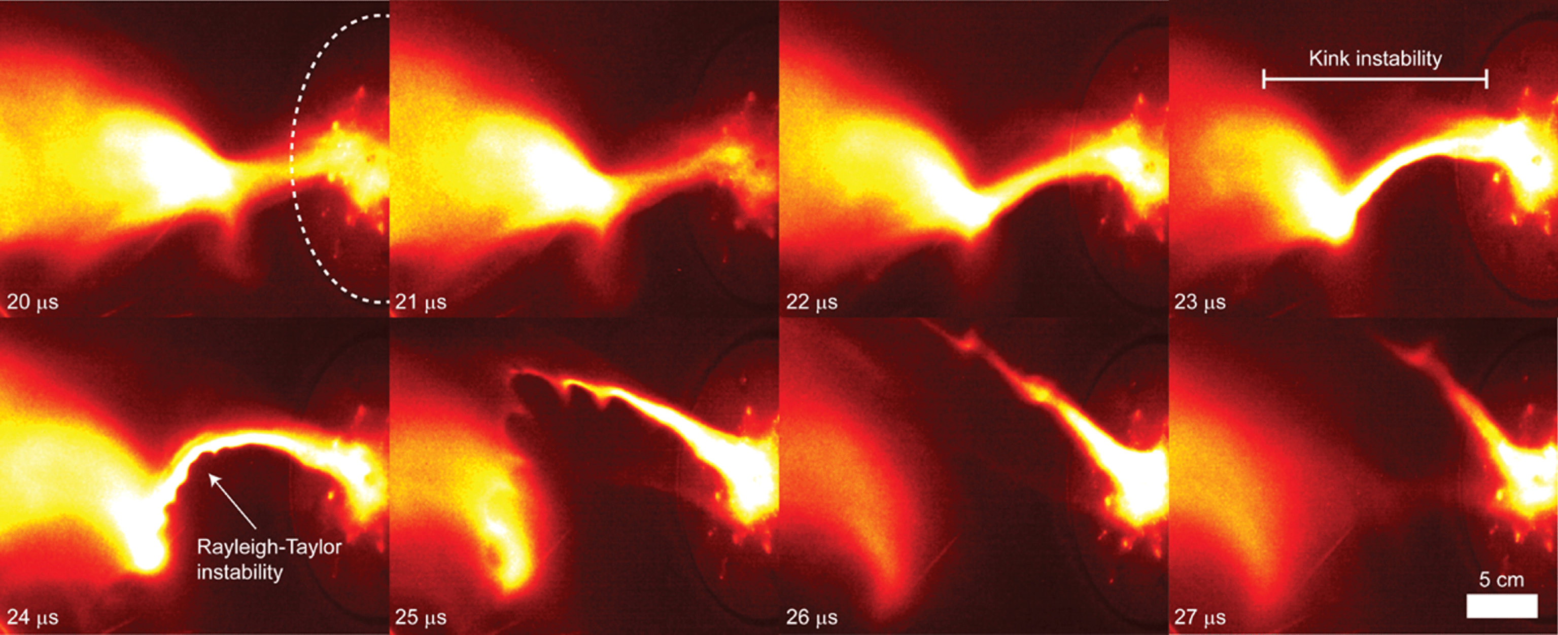
Figure 9. Kink instigation of a Rayleigh–Taylor instability. Disk electrode location shown as dotted circle in top left frame and the jet travels from right to left. The top right frame shows the kink wavelength while the bottom left frame shows the development of Rayleigh–Taylor ripples. These ripples grow by a factor of
 $e$
in one frame and so the Rayleigh–Taylor instability is much faster than the kink. [Figure reproduced from Moser and Bellan, Nature 482, 379 (2012).]
$e$
in one frame and so the Rayleigh–Taylor instability is much faster than the kink. [Figure reproduced from Moser and Bellan, Nature 482, 379 (2012).]
The standard model of the RTI assumes Cartesian geometry where the heavy fluid lies above a plane and the light fluid lies below this plane so that ripples develop at the planar interface. The jet situation is geometrically more complex because the jet has a round cross-section so the RTI effectively occurs on the bottom of a horizontally aligned cylinder. Because of this more complex geometry, it is expected that the standard planar model will only predict the general tendency but not the detailed dependence. In particular, the standard planar model is incapable of determining the relationship between the ripple wavelength and the jet diameter since the planar model effectively assumes infinite jet diameter. Zhai & Bellan (Reference Zhai and Bellan2016) developed a model for the RTI in the case of a cylindrical plasma undergoing lateral acceleration so that the ripples occur on the bottom of the cylinder where bottom is defined with respect to the direction of the effective gravity. This model calculates the coupling between a large number of azimuthal Fourier modes and so can characterize situations where an instability occurs only at the cylinder bottom. Moser & Bellan (Reference Moser and Bellan2012a ) observed strong RTI in argon plasma jets but only observed RTI in hydrogen plasma jets on rare occasions and, when observed, the RTI was much weaker than for the argon jets. Zhai & Bellan (Reference Zhai and Bellan2016) also observed this difference between argon and hydrogen jets in experiments and resolved the difference in more detail as shown in figure 10.
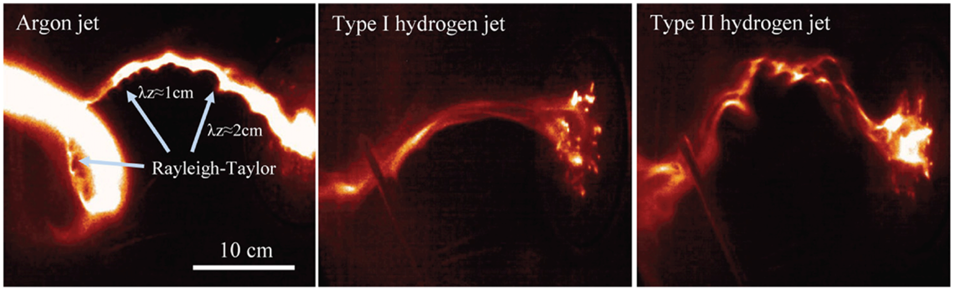
Figure 10. Difference between argon and hydrogen jets. Argon jet has
 $g=4\times 10^{10}~\text{m}~\text{s}^{-2}$
and shows clear evidence of Rayleigh–Taylor ripples superimposed on much longer wavelength helical kink instability. Type I hydrogen jet has
$g=4\times 10^{10}~\text{m}~\text{s}^{-2}$
and shows clear evidence of Rayleigh–Taylor ripples superimposed on much longer wavelength helical kink instability. Type I hydrogen jet has
 $g=3\times 10^{10}~\text{m}~\text{s}^{-2}$
, kinks, but has no Rayleigh–Taylor instability. Type II hydrogen jet has much larger effective gravity of
$g=3\times 10^{10}~\text{m}~\text{s}^{-2}$
, kinks, but has no Rayleigh–Taylor instability. Type II hydrogen jet has much larger effective gravity of
 $g=1.5\times 10^{11}~\text{m}~\text{s}^{-2}$
, kinks, but exhibits a secondary instability that has both Rayleigh–Taylor and fine-scale kink properties, namely ripples and a helical shape. [Reprinted from Zhai and Bellan, Physics of Plasmas 23, 032121 (2016) with the permission of AIP Publishing.]
$g=1.5\times 10^{11}~\text{m}~\text{s}^{-2}$
, kinks, but exhibits a secondary instability that has both Rayleigh–Taylor and fine-scale kink properties, namely ripples and a helical shape. [Reprinted from Zhai and Bellan, Physics of Plasmas 23, 032121 (2016) with the permission of AIP Publishing.]
RTI growth rates in good agreement with observations for hydrogen and argon jets were predicted by Zhai & Bellan (Reference Zhai and Bellan2016) as well as the wavelength of the fastest growing ripple. The model decomposes the instability into a superposition of azimuthal components each varying as
 $\exp (\text{i}m\unicode[STIX]{x1D719})$
and shows that the lack of azimuthal symmetry resulting from the one-sided push leads to a complicated coupling between the different
$\exp (\text{i}m\unicode[STIX]{x1D719})$
and shows that the lack of azimuthal symmetry resulting from the one-sided push leads to a complicated coupling between the different
 $m$
modes. Solving for the dynamics involves inverting an infinite matrix coupling the
$m$
modes. Solving for the dynamics involves inverting an infinite matrix coupling the
 $m$
modes to each other. The analysis further shows that there is a continuum of behaviour between kink and Rayleigh–Taylor instabilities where the kink here is a secondary instability not to be confused with the primary kink instability that is providing the effective gravity. The parameter space is characterized by the dimensionless quantity
$m$
modes to each other. The analysis further shows that there is a continuum of behaviour between kink and Rayleigh–Taylor instabilities where the kink here is a secondary instability not to be confused with the primary kink instability that is providing the effective gravity. The parameter space is characterized by the dimensionless quantity
 $\unicode[STIX]{x1D6F7}=ga/v_{A\unicode[STIX]{x1D719}}^{2}$
where
$\unicode[STIX]{x1D6F7}=ga/v_{A\unicode[STIX]{x1D719}}^{2}$
where
 $g$
is the gravity from the lateral acceleration,
$g$
is the gravity from the lateral acceleration,
 $a$
is the radius of the cylindrical flux tube (i.e. jet radius), and
$a$
is the radius of the cylindrical flux tube (i.e. jet radius), and
 $v_{A\unicode[STIX]{x1D719}}^{2}$
is the Alfvén velocity calculated using the azimuthal magnetic field. If
$v_{A\unicode[STIX]{x1D719}}^{2}$
is the Alfvén velocity calculated using the azimuthal magnetic field. If
 $\unicode[STIX]{x1D6F7}\ll 1$
then gravity is negligible and the secondary instability is a pure kink with a narrow spectrum of azimuthal modes as shown in figure 11 whereas if
$\unicode[STIX]{x1D6F7}\ll 1$
then gravity is negligible and the secondary instability is a pure kink with a narrow spectrum of azimuthal modes as shown in figure 11 whereas if
 $\unicode[STIX]{x1D6F7}\gg 1$
the instability is pure Rayleigh–Taylor with a broad spectrum of azimuthal modes as also shown in figure 11. The broad Fourier mode spectrum is required to have the instability azimuthally localized to the bottom of the cylinder. When
$\unicode[STIX]{x1D6F7}\gg 1$
the instability is pure Rayleigh–Taylor with a broad spectrum of azimuthal modes as also shown in figure 11. The broad Fourier mode spectrum is required to have the instability azimuthally localized to the bottom of the cylinder. When
 $\unicode[STIX]{x1D6F7}$
is of order unity, the instability has properties of both kink and Rayleigh–Taylor. Because
$\unicode[STIX]{x1D6F7}$
is of order unity, the instability has properties of both kink and Rayleigh–Taylor. Because
 $v_{A\unicode[STIX]{x1D719}}^{2}=B_{\unicode[STIX]{x1D719}}^{2}/\unicode[STIX]{x1D707}_{0}\unicode[STIX]{x1D70C}$
, the situation where
$v_{A\unicode[STIX]{x1D719}}^{2}=B_{\unicode[STIX]{x1D719}}^{2}/\unicode[STIX]{x1D707}_{0}\unicode[STIX]{x1D70C}$
, the situation where
 $\unicode[STIX]{x1D6F7}$
is of order unity is mass dependent such that
$\unicode[STIX]{x1D6F7}$
is of order unity is mass dependent such that
 $\unicode[STIX]{x1D6F7}$
is proportional to mass which means that all other parameters being equal, heavy jets are more susceptible to the RTI than light jets. This was observed experimentally as argon jets always had RTI whereas hydrogen jets only exhibited RTI when there was extreme acceleration and furthermore the hydrogen jet RTI showed some kink-like characteristics associated with having a narrow azimuthal mode spectrum. Figure 12 compares the predicted argon structure (broad azimuthal mode spectrum, perturbation concentrated at an azimuthal location corresponding to the bottom and so giving ripples) to the hydrogen structure (narrow azimuthal mode spectrum, perturbation having only slight localization at the bottom and so giving a more helical, kink-like structure). This is in good agreement with the observations shown in figure 10 where it is seen that the argon jet has a Rayleigh–Taylor ripple structure whereas the Type II hydrogen jet has a secondary instability that is more kink-like.
$\unicode[STIX]{x1D6F7}$
is proportional to mass which means that all other parameters being equal, heavy jets are more susceptible to the RTI than light jets. This was observed experimentally as argon jets always had RTI whereas hydrogen jets only exhibited RTI when there was extreme acceleration and furthermore the hydrogen jet RTI showed some kink-like characteristics associated with having a narrow azimuthal mode spectrum. Figure 12 compares the predicted argon structure (broad azimuthal mode spectrum, perturbation concentrated at an azimuthal location corresponding to the bottom and so giving ripples) to the hydrogen structure (narrow azimuthal mode spectrum, perturbation having only slight localization at the bottom and so giving a more helical, kink-like structure). This is in good agreement with the observations shown in figure 10 where it is seen that the argon jet has a Rayleigh–Taylor ripple structure whereas the Type II hydrogen jet has a secondary instability that is more kink-like.
Figure 11. Azimuthal mode spectrum for argon and hydrogen situations. The hydrogen spectrum is narrow and is almost a single mode which corresponds to the kink-like helical behaviour. The argon spectrum is broad and so contains sufficient modes to produce a delta-function profile in
 $\unicode[STIX]{x1D719}$
space, corresponding to ripples on the cylinder bottom but not at other angles. [Reprinted from Zhai and Bellan, Physics of Plasmas 23, 032121 (2016) with the permission of AIP Publishing.]
$\unicode[STIX]{x1D719}$
space, corresponding to ripples on the cylinder bottom but not at other angles. [Reprinted from Zhai and Bellan, Physics of Plasmas 23, 032121 (2016) with the permission of AIP Publishing.]

Figure 12. Top shows superimposed azimuthal modes for argon jet and bottom shows similar for hydrogen jet. The broad mode spectrum for argon enables the perturbation to be highly localized at one azimuthal angle (i.e., the bottom) whereas the broad hydrogen mode spectrum provides only a small amount of localizations. [Reprinted from Zhai and Bellan, Physics of Plasmas 23, 032121 (2016) with the permission of AIP Publishing.]
7 Consequences of the Rayleigh–Taylor instability
The RTI is observed to instigate several associated phenomena that have significant effects on the jet. These phenomena appear to be associated with the one-sided nature of the RTI as ripples develop only on the trailing side of the laterally accelerated jet because only on this side is there a heavy fluid effectively on top of a light fluid. The one-sided nature of the ripples means that the jet cross-section is constricted where the ripples eat into the jet; this constriction means that there will be an increase of the axial electric current density in the jet. It is observed that when the jet cross-section becomes sufficiently constricted to be of the order of the ion skin depth
 $d_{i}=c/\unicode[STIX]{x1D714}_{pi}$
, the jet appears to break. High speed movies of both the visible and extreme ultra-violet (EUV) optical emission from the jet show that there is dimming of the visible emission and an enhancement of the EUV emission (Chai, Zhai & Bellan Reference Chai, Zhai and Bellan2016) at the RTI location. This suggests that there is a substantial density depletion at the RTI location as visible emission scales as the square of the density. This also suggests that there is a substantial heating of the electrons in the remaining density since hot electrons are required to excite bound electrons in the remaining ions to high enough energy states to have strong EUV emission. Additional evidence for the existence of energetic electrons is a change in the nature of the emitted atomic line spectrum. Before the RTI occurs, the observed atomic lines are mainly from singly ionized argon with negligible neutral emission and negligible emission from doubly ionized argon or from higher ionized states. However, during the RTI the line emission is primarily from doubly ionized argon and there is some emission from triply ionized argon. This change in emission spectra indicates that the electrons have been substantially heated during the RTI. The width of the ion lines also increases indicating that there is ion heating as well. Measurements of high frequency magnetic oscillations show an onset of such oscillations when the RTI occurs suggesting that the RTI also instigates generation of waves (Chai et al.
Reference Chai, Zhai and Bellan2016).
$d_{i}=c/\unicode[STIX]{x1D714}_{pi}$
, the jet appears to break. High speed movies of both the visible and extreme ultra-violet (EUV) optical emission from the jet show that there is dimming of the visible emission and an enhancement of the EUV emission (Chai, Zhai & Bellan Reference Chai, Zhai and Bellan2016) at the RTI location. This suggests that there is a substantial density depletion at the RTI location as visible emission scales as the square of the density. This also suggests that there is a substantial heating of the electrons in the remaining density since hot electrons are required to excite bound electrons in the remaining ions to high enough energy states to have strong EUV emission. Additional evidence for the existence of energetic electrons is a change in the nature of the emitted atomic line spectrum. Before the RTI occurs, the observed atomic lines are mainly from singly ionized argon with negligible neutral emission and negligible emission from doubly ionized argon or from higher ionized states. However, during the RTI the line emission is primarily from doubly ionized argon and there is some emission from triply ionized argon. This change in emission spectra indicates that the electrons have been substantially heated during the RTI. The width of the ion lines also increases indicating that there is ion heating as well. Measurements of high frequency magnetic oscillations show an onset of such oscillations when the RTI occurs suggesting that the RTI also instigates generation of waves (Chai et al.
Reference Chai, Zhai and Bellan2016).
The working hypothesis at the present time (Marshall & Bellan Reference Marshall and Bellan2017) is that the increase of electric current density
 $\boldsymbol{J}$
as a result of the RTI constricting the jet cross-section means that the electron drift velocity
$\boldsymbol{J}$
as a result of the RTI constricting the jet cross-section means that the electron drift velocity
 $v_{d}=J/ne$
with respect to ions increases. When
$v_{d}=J/ne$
with respect to ions increases. When
 $v_{d}$
becomes comparable to some characteristic wave phase velocity, the ions can be considered as a mono-energetic beam flowing at this velocity through the electrons. Such a beam is unstable with respect to kinetic beam instabilities and so a rapidly growing kinetic instability develops. This instability tends to scatter electrons and so acts as an effective resistivity. The net effect is that the RTI causes the plasma to become highly resistive compared to before the RTI and so the RTI location can be considered as being like an opening switch in an electric circuit. Since the remaining part of the circuit has substantial inductance, the opening switch is in series with an inductive circuit. There will be a large inductive voltage at the location of the opening switch and the electric field associated with this voltage drop will accelerate electrons to high energy.
$v_{d}$
becomes comparable to some characteristic wave phase velocity, the ions can be considered as a mono-energetic beam flowing at this velocity through the electrons. Such a beam is unstable with respect to kinetic beam instabilities and so a rapidly growing kinetic instability develops. This instability tends to scatter electrons and so acts as an effective resistivity. The net effect is that the RTI causes the plasma to become highly resistive compared to before the RTI and so the RTI location can be considered as being like an opening switch in an electric circuit. Since the remaining part of the circuit has substantial inductance, the opening switch is in series with an inductive circuit. There will be a large inductive voltage at the location of the opening switch and the electric field associated with this voltage drop will accelerate electrons to high energy.
8 Numerical simulation compared to experiment
Zhai et al. (Reference Zhai, Li, Bellan and Li2014) modelled the Caltech jet experiment using a three-dimensional numerical MHD code. This code, originally developed to model astrophysical jets, was modified to incorporate the boundary conditions and parameters of the Caltech experiment. The code results were quite similar to the experimental observations and support the analytic interpretations presented here. In particular, synthetic movies made from the code were very similar to movies of the actual experiment. The synthetic movies showed the line average of the square of the density which is the quantity measured by a camera in the actual experiment since the optical emission scales as density squared and the jet is optically thin so the image is a line average.
An important realization resulting from the construction of the numerical simulation code was that ideal MHD is incapable of modelling the experimental boundary conditions. This is because these boundary conditions involve injection of magnetic flux at the boundary whereas ideal MHD does not permit injection of magnetic flux. Thus, a localized fictitious non-ideal region had to be inserted to model the flux injection at the electrodes. Specifically, the MHD induction equation (2.2) had a non-physical term added to the right hand side such that this term acted as a localized source of magnetic flux. The non-physical term was located just below the
 $z=0$
plane so the physical region, i.e. positive
$z=0$
plane so the physical region, i.e. positive
 $z$
region, excluded this fictitious source. This scheme allowed for injection of toroidal magnetic flux into the physical region, i.e. driving a poloidal current going from the inner to outer electrode. However, this raised the question of what happens in a real astrophysical jet and suggested that the source region of a real astrophysical jet must involve physics beyond the realm of ideal MHD. This non-MHD physics is discussed in § 10.
$z$
region, excluded this fictitious source. This scheme allowed for injection of toroidal magnetic flux into the physical region, i.e. driving a poloidal current going from the inner to outer electrode. However, this raised the question of what happens in a real astrophysical jet and suggested that the source region of a real astrophysical jet must involve physics beyond the realm of ideal MHD. This non-MHD physics is discussed in § 10.
9 Jet–cloud collision experiment
The collision of an MHD-driven jet with a target cloud has been investigated in the experiments (Moser & Bellan Reference Moser and Bellan2012b ; Seo & Bellan Reference Seo and Bellan2017). This investigation involves injecting a cloud of neutral gas in the path of the jet. The cloud is injected using a fast pulsed gas valve and the cloud location at the time the jet impacts the cloud can be adjusted by changing the time at which the fast gas valve opens. The fast gas valve is connected to a metal tube aligned to point towards the jet so the injected cloud travels towards the jet. The cloud velocity is just the thermal velocity of room temperature gas, i.e. a few hundred metres per second whereas the jet velocity is tens of kilometres per second. Thus, the cloud is effectively a stationary target for the jet.
Having a hydrogen jet impact an argon cloud causes an abrupt decrease in the jet velocity and a simultaneous increase of the density of the jet at the stagnation region. This has been measured using a translatable laser interferometer that measures the plasma density as a function of both axial position and time (Seo & Bellan Reference Seo and Bellan2017). Figure 13 shows a plot from Seo & Bellan (Reference Seo and Bellan2017) of the line-averaged density
 $n(z,t)$
for the situation where a jet collides with a target cloud located at 280 mm. The velocity, determined from the slope of the red dashed line, is initially
$n(z,t)$
for the situation where a jet collides with a target cloud located at 280 mm. The velocity, determined from the slope of the red dashed line, is initially
 $70~\text{km}~\text{s}^{-1}$
but slows to
$70~\text{km}~\text{s}^{-1}$
but slows to
 $20~\text{km}~\text{s}^{-1}$
at 280 mm where the jet impacts the target cloud and the jet density increases. The slowing down is presumed to be collisional because the collisional mean free path is small compared to the physical dimensions. However, the electric currents and the magnetic flux are largely maintained as their minimal dissipation is related to the large Lundquist number in the experiment. This flux conservation is observed as an approximately twofold amplification of the magnetic field in the jet tip which is compressed as it collides with the cloud (Moser & Bellan Reference Moser and Bellan2012b
); the magnetic field amplification corresponds to an increase of the magnetic flux density as a result of the compression. This compression and field amplification should be relevant to the situation of an astrophysical jet colliding with a molecular cloud as such a collision also involves a large Lundquist number together with a collisional mean free path small compared to the system dimensions.
$20~\text{km}~\text{s}^{-1}$
at 280 mm where the jet impacts the target cloud and the jet density increases. The slowing down is presumed to be collisional because the collisional mean free path is small compared to the physical dimensions. However, the electric currents and the magnetic flux are largely maintained as their minimal dissipation is related to the large Lundquist number in the experiment. This flux conservation is observed as an approximately twofold amplification of the magnetic field in the jet tip which is compressed as it collides with the cloud (Moser & Bellan Reference Moser and Bellan2012b
); the magnetic field amplification corresponds to an increase of the magnetic flux density as a result of the compression. This compression and field amplification should be relevant to the situation of an astrophysical jet colliding with a molecular cloud as such a collision also involves a large Lundquist number together with a collisional mean free path small compared to the system dimensions.

Figure 13. Density (colour) as function of time and position. The jet velocity is given by the slope of the high density crest which is highlighted by the red dotted line. The jet collides with a target cloud at 280 mm. The slope decreases indicating slowing down of the jet and the density increases (yellow region). The density scale (color bar on right) is in units of
 $\text{m}^{-3}$
. [Reprinted from Seo and Bellan, Review of Scientific Instruments 88, 123504 (2017) with the permission of AIP Publishing.]
$\text{m}^{-3}$
. [Reprinted from Seo and Bellan, Review of Scientific Instruments 88, 123504 (2017) with the permission of AIP Publishing.]
10 Accretion disk launching of jets

Figure 14. Laboratory layout. Gas is injected from both the disk and the annulus. [Figure from Bellan, Monthly Notices Royal Astronomical Society 458, 4400 (2016).]
As discussed in Bellan (Reference Bellan2016a
) the laboratory experiment layout sketched in figure 14 could conceivably be reflected to be as in figure 15 so as to have bidirectional jets originating from a common power supply and common mass source. Figure 15 is analogous to the sketch of an accretion disk launching bidirectional astrophysical jets shown in figure 16. Consideration of the symmetry and boundary conditions relating these sketches shows that the accretion disk must provide a mass source for the bidirectional jets and that the accretion disk must also act as an electrical power supply that drives the poloidal electric current flowing in the jets. The poloidal flux would have to be a symmetric function of
 $z$
and the poloidal current would have to be an antisymmetric function of
$z$
and the poloidal current would have to be an antisymmetric function of
 $z$
, i.e.
$z$
, i.e.
 $\unicode[STIX]{x1D713}(r,-z,t)=\unicode[STIX]{x1D713}(r,z,t)$
and
$\unicode[STIX]{x1D713}(r,-z,t)=\unicode[STIX]{x1D713}(r,z,t)$
and
 $I(r,-z,t)=-I(r,z,t)$
. These symmetries are such that
$I(r,-z,t)=-I(r,z,t)$
. These symmetries are such that
 $(\boldsymbol{J}\times \boldsymbol{B})_{r}$
is symmetric with respect to
$(\boldsymbol{J}\times \boldsymbol{B})_{r}$
is symmetric with respect to
 $z$
while
$z$
while
 $(\boldsymbol{J}\times \boldsymbol{B})_{z}$
is antisymmetric with respect to
$(\boldsymbol{J}\times \boldsymbol{B})_{z}$
is antisymmetric with respect to
 $z;$
this can be verified by consideration of the magnetic terms on the right hand sides of (2.24a
) and (2.24c
). These symmetries provide radial confinement for both positive and negative
$z;$
this can be verified by consideration of the magnetic terms on the right hand sides of (2.24a
) and (2.24c
). These symmetries provide radial confinement for both positive and negative
 $z$
while also accelerating bidirectional jets away from the
$z$
while also accelerating bidirectional jets away from the
 $z=0$
plane.
$z=0$
plane.
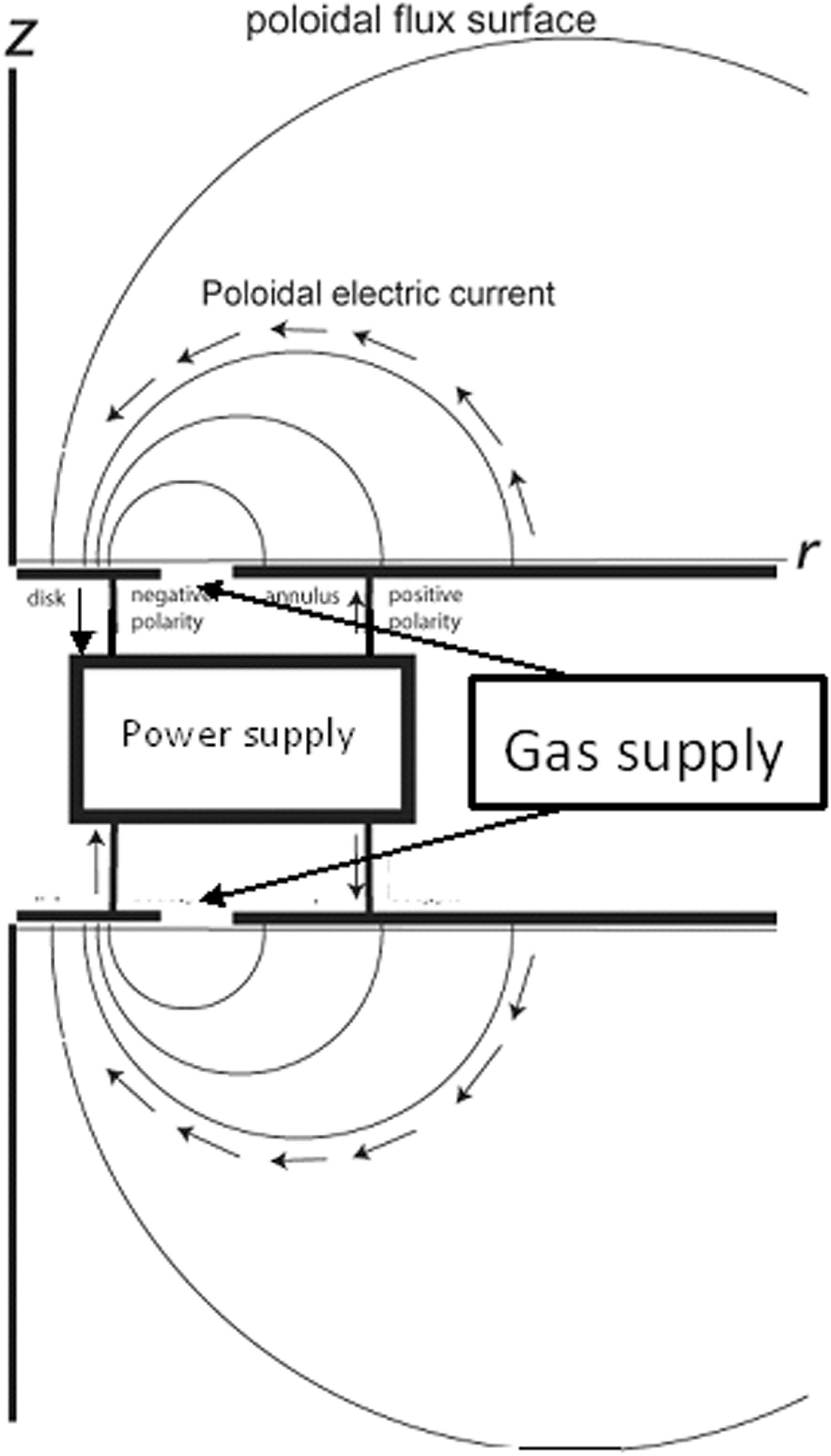
Figure 15. Laboratory set-up and reflection.

Figure 16. Sketch of astrophysical jet. Reproduced from Paul M. Bellan, Plasma Phys. Control. Fusion 60, 014006 (2018). © IOP Publishing Ltd. CC BY 3.0.
In order to sustain the outward mass flux from the
 $z=0$
plane there must be a radially inward mass flux in the
$z=0$
plane there must be a radially inward mass flux in the
 $z=0$
plane. This would come from a portion of the mass accreting onto the accretion disk and corresponds to the gas injection in the laboratory experiment. However, a quasi-steady radially inward motion of plasma in the
$z=0$
plane. This would come from a portion of the mass accreting onto the accretion disk and corresponds to the gas injection in the laboratory experiment. However, a quasi-steady radially inward motion of plasma in the
 $z=0$
plane is not consistent with ideal MHD. This is because the jet motion involves distending poloidal flux that is anchored in the accretion disk, i.e. anchored in the
$z=0$
plane is not consistent with ideal MHD. This is because the jet motion involves distending poloidal flux that is anchored in the accretion disk, i.e. anchored in the
 $z=0$
plane. Since
$z=0$
plane. Since
 $E_{\unicode[STIX]{x1D719}}=-r^{-1}\unicode[STIX]{x2202}V/\unicode[STIX]{x2202}\unicode[STIX]{x1D719}-(2\unicode[STIX]{x03C0}r)^{-1}\unicode[STIX]{x2202}\unicode[STIX]{x1D713}/\unicode[STIX]{x2202}t$
where
$E_{\unicode[STIX]{x1D719}}=-r^{-1}\unicode[STIX]{x2202}V/\unicode[STIX]{x2202}\unicode[STIX]{x1D719}-(2\unicode[STIX]{x03C0}r)^{-1}\unicode[STIX]{x2202}\unicode[STIX]{x1D713}/\unicode[STIX]{x2202}t$
where
 $V$
is an electrostatic potential, the symmetry in
$V$
is an electrostatic potential, the symmetry in
 $\unicode[STIX]{x1D719}$
and invariance of
$\unicode[STIX]{x1D719}$
and invariance of
 $\unicode[STIX]{x1D713}$
in the
$\unicode[STIX]{x1D713}$
in the
 $z=0$
plane show that
$z=0$
plane show that
 $E_{\unicode[STIX]{x1D719}}=0$
in the
$E_{\unicode[STIX]{x1D719}}=0$
in the
 $z=0$
plane. Since the jets are bidirectional,
$z=0$
plane. Since the jets are bidirectional,
 $U_{z}=0$
in the
$U_{z}=0$
in the
 $z=0$
plane. Because
$z=0$
plane. Because
 $\unicode[STIX]{x1D713}$
is finite in the
$\unicode[STIX]{x1D713}$
is finite in the
 $z=0$
plane,
$z=0$
plane,
 $\unicode[STIX]{x2202}\unicode[STIX]{x1D713}/\unicode[STIX]{x2202}r$
and hence
$\unicode[STIX]{x2202}\unicode[STIX]{x1D713}/\unicode[STIX]{x2202}r$
and hence
 $B_{z}$
is finite in the
$B_{z}$
is finite in the
 $z=0$
plane. Finally, accretion means that
$z=0$
plane. Finally, accretion means that
 $U_{r}$
is finite and negative in the
$U_{r}$
is finite and negative in the
 $z=0$
plane. The azimuthal component of the ideal MHD Ohm’s law is
$z=0$
plane. The azimuthal component of the ideal MHD Ohm’s law is
 $$\begin{eqnarray}E_{\unicode[STIX]{x1D719}}+U_{z}B_{r}-U_{r}B_{z}=0\end{eqnarray}$$
and it is seen that only the last term, i.e.
 $-U_{r}B_{z}$
, is finite in this equation in the
$-U_{r}B_{z}$
, is finite in this equation in the
 $z=0$
plane. Because only one term is finite it is impossible to satisfy this equation in the
$z=0$
plane. Because only one term is finite it is impossible to satisfy this equation in the
 $z=0$
plane and so in the
$z=0$
plane and so in the
 $z=0$
plane ideal MHD cannot describe the plasma flow and magnetic symmetries prescribed above.
$z=0$
plane ideal MHD cannot describe the plasma flow and magnetic symmetries prescribed above.
Equation (10.1) is just (2.53) as can be seen using (2.28) and (2.29). In the
 $z=0$
plane
$z=0$
plane
 $U_{z}=0$
by symmetry so (2.53) would then reduce in the
$U_{z}=0$
by symmetry so (2.53) would then reduce in the
 $z=0$
plane to
$z=0$
plane to
 $$\begin{eqnarray}\frac{\unicode[STIX]{x2202}\unicode[STIX]{x1D713}}{\unicode[STIX]{x2202}t}+U_{r}\frac{\unicode[STIX]{x2202}\unicode[STIX]{x1D713}}{\unicode[STIX]{x2202}r}=0\end{eqnarray}$$
and using
 $\unicode[STIX]{x1D713}=B_{z}\unicode[STIX]{x03C0}r^{2}$
at small
$\unicode[STIX]{x1D713}=B_{z}\unicode[STIX]{x03C0}r^{2}$
at small
 $r$
, this would give
$r$
, this would give
 $$\begin{eqnarray}\frac{\unicode[STIX]{x2202}B_{z}}{\unicode[STIX]{x2202}t}+2\frac{U_{r}}{r}B_{z}=0,\end{eqnarray}$$
which would lead to a non-physical unbounded exponential growth of
 $B_{z}$
if
$B_{z}$
if
 $U_{r}$
is negative, i.e. if there is accretion. Besides showing why the ideal MHD Ohm’s law is incompatible with an accretion disk linked by a constant poloidal flux, this analysis also shows why a poloidal field stabilizes the sausage (necking) instability in a
$U_{r}$
is negative, i.e. if there is accretion. Besides showing why the ideal MHD Ohm’s law is incompatible with an accretion disk linked by a constant poloidal flux, this analysis also shows why a poloidal field stabilizes the sausage (necking) instability in a
 $Z$
-pinch since the necking (inward
$Z$
-pinch since the necking (inward
 $U_{r}$
) would result in an infinite amplification of
$U_{r}$
) would result in an infinite amplification of
 $B_{z}$
. Instead of the magnetic energy decreasing as required for an instability, the magnetic energy would become infinite.
$B_{z}$
. Instead of the magnetic energy decreasing as required for an instability, the magnetic energy would become infinite.
The requirement that steady-state electric current must flow nearly along poloidal flux surfaces depends on the poloidal Larmor radius being microscopic. If the poloidal Larmor radius becomes comparable to the system size, then particles can flow across poloidal flux surfaces. Having an extremely large poloidal Larmor radius corresponds to having an extremely small charge-to-mass ratio. The author showed in Bellan (Reference Bellan2007, Reference Bellan2008, Reference Bellan2016a
,Reference Bellan
b
, Reference Bellan2017) that, if for some reason, the two terms in (2.26) have the same magnitude and are equal and opposite, then charged particles can cross poloidal flux surfaces and in the presence of gravity will spiral in towards the origin. This situation is not required for all the particles and in fact it is envisaged that only a tiny subset would have
 $P_{\unicode[STIX]{x1D719}}=0$
. The relative scaling of the two terms in (2.26) can be seen by writing
$P_{\unicode[STIX]{x1D719}}=0$
. The relative scaling of the two terms in (2.26) can be seen by writing
 $v_{\unicode[STIX]{x1D719}}=r\dot{\unicode[STIX]{x1D719}}$
and
$v_{\unicode[STIX]{x1D719}}=r\dot{\unicode[STIX]{x1D719}}$
and
 $\unicode[STIX]{x1D713}\sim B_{z}\unicode[STIX]{x03C0}r^{2}$
so the two terms scale as
$\unicode[STIX]{x1D713}\sim B_{z}\unicode[STIX]{x03C0}r^{2}$
so the two terms scale as
 $$\begin{eqnarray}mr^{2}\dot{\unicode[STIX]{x1D719}}:\frac{qB_{z}}{2}r^{2}\end{eqnarray}$$
or as
 $$\begin{eqnarray}\dot{\unicode[STIX]{x1D719}}:\unicode[STIX]{x1D714}_{c},\end{eqnarray}$$
where
 $\unicode[STIX]{x1D714}_{c}=qB_{z}/m$
is the cyclotron frequency and
$\unicode[STIX]{x1D714}_{c}=qB_{z}/m$
is the cyclotron frequency and
 $\dot{\unicode[STIX]{x1D719}}$
is assumed to be of the order of the Kepler angular velocity since it is presumed that an accretion disk is undergoing Kepler orbital motion. Since cyclotron frequencies are typically many orders of magnitude larger than Kepler frequencies, the second term in (2.26) is normally many orders of magnitude larger than the first term. However, if for some reason the effective charge-to-mass ratio
$\dot{\unicode[STIX]{x1D719}}$
is assumed to be of the order of the Kepler angular velocity since it is presumed that an accretion disk is undergoing Kepler orbital motion. Since cyclotron frequencies are typically many orders of magnitude larger than Kepler frequencies, the second term in (2.26) is normally many orders of magnitude larger than the first term. However, if for some reason the effective charge-to-mass ratio
 $q/m$
is reduced so that
$q/m$
is reduced so that
 $\unicode[STIX]{x1D714}_{c}$
becomes of the order of the Kepler frequency there will be a strong interaction between the magnetic and gravitational forces and the resulting motion will be neither a Kepler orbit nor a cyclotron orbit.
$\unicode[STIX]{x1D714}_{c}$
becomes of the order of the Kepler frequency there will be a strong interaction between the magnetic and gravitational forces and the resulting motion will be neither a Kepler orbit nor a cyclotron orbit.
As both Kepler and cyclotron orbits are single-particle motions, it is necessary to examine the motion using single-particle theory. Since we are interested in behaviour in the
 $z=0$
plane, we first consider the situation of a particle in this plane subject to a magnetic field in the
$z=0$
plane, we first consider the situation of a particle in this plane subject to a magnetic field in the
 $z$
direction and to a gravitational field in the radial direction. The Lagrangian in this situation is
$z$
direction and to a gravitational field in the radial direction. The Lagrangian in this situation is
 $$\begin{eqnarray}{\mathcal{L}}=\frac{1}{2}m(v_{r}^{2}+r^{2}\dot{\unicode[STIX]{x1D719}}^{2})+qr\dot{\unicode[STIX]{x1D719}}A_{\unicode[STIX]{x1D719}}+\frac{mMG}{r}\end{eqnarray}$$
and the associated Hamiltonian is
 $$\begin{eqnarray}H=\frac{1}{2}m(v_{r}^{2}+r^{2}\dot{\unicode[STIX]{x1D719}}^{2})-\frac{mMG}{r}.\end{eqnarray}$$
The canonical angular momentum defined as
 $P_{\unicode[STIX]{x1D719}}=\unicode[STIX]{x2202}{\mathcal{L}}/\unicode[STIX]{x2202}\dot{\unicode[STIX]{x1D719}}$
is given by (2.26) where
$P_{\unicode[STIX]{x1D719}}=\unicode[STIX]{x2202}{\mathcal{L}}/\unicode[STIX]{x2202}\dot{\unicode[STIX]{x1D719}}$
is given by (2.26) where
 $\unicode[STIX]{x1D713}=2\unicode[STIX]{x03C0}rA_{\unicode[STIX]{x1D719}}$
has been used as seen from
$\unicode[STIX]{x1D713}=2\unicode[STIX]{x03C0}rA_{\unicode[STIX]{x1D719}}$
has been used as seen from
 $B_{z}=r^{-1}\unicode[STIX]{x2202}/\unicode[STIX]{x2202}r(rA_{\unicode[STIX]{x1D719}})=(2\unicode[STIX]{x03C0}r)^{-1}\unicode[STIX]{x2202}\unicode[STIX]{x1D713}/\unicode[STIX]{x2202}r$
. The Hamiltonian can be expressed as
$B_{z}=r^{-1}\unicode[STIX]{x2202}/\unicode[STIX]{x2202}r(rA_{\unicode[STIX]{x1D719}})=(2\unicode[STIX]{x03C0}r)^{-1}\unicode[STIX]{x2202}\unicode[STIX]{x1D713}/\unicode[STIX]{x2202}r$
. The Hamiltonian can be expressed as
 $$\begin{eqnarray}H={\textstyle \frac{1}{2}}mv_{r}^{2}+\unicode[STIX]{x1D712}(r),\end{eqnarray}$$
where
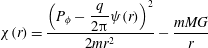 $$\begin{eqnarray}\unicode[STIX]{x1D712}(r)=\frac{\left(P_{\unicode[STIX]{x1D719}}-{\displaystyle \frac{q}{2\unicode[STIX]{x03C0}}}\unicode[STIX]{x1D713}(r)\right)^{2}}{2mr^{2}}-\frac{mMG}{r}\end{eqnarray}$$
is an effective potential. If there is no magnetic field then
 $\unicode[STIX]{x1D713}=0$
in which case
$\unicode[STIX]{x1D713}=0$
in which case
 $\unicode[STIX]{x1D712}$
becomes the Kepler effective potential and the particle executes Kepler orbits. If there is no gravity, then
$\unicode[STIX]{x1D712}$
becomes the Kepler effective potential and the particle executes Kepler orbits. If there is no gravity, then
 $\unicode[STIX]{x1D712}$
is the effective potential for cyclotron orbits (Schmidt Reference Schmidt1979; Bellan Reference Bellan2006). If
$\unicode[STIX]{x1D712}$
is the effective potential for cyclotron orbits (Schmidt Reference Schmidt1979; Bellan Reference Bellan2006). If
 $P_{\unicode[STIX]{x1D719}}=0$
there exists a qualitatively different, intermediate type of orbit that is neither Kepler nor cyclotron. In the
$P_{\unicode[STIX]{x1D719}}=0$
there exists a qualitatively different, intermediate type of orbit that is neither Kepler nor cyclotron. In the
 $P_{\unicode[STIX]{x1D719}}=0$
situation, the effective potential reduces to
$P_{\unicode[STIX]{x1D719}}=0$
situation, the effective potential reduces to
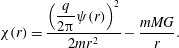 $$\begin{eqnarray}\unicode[STIX]{x1D712}(r)=\frac{\left({\displaystyle \frac{q}{2\unicode[STIX]{x03C0}}}\unicode[STIX]{x1D713}(r)\right)^{2}}{2mr^{2}}-\frac{mMG}{r}.\end{eqnarray}$$
At small
 $r$
, mathematical regularity requires
$r$
, mathematical regularity requires
 $\unicode[STIX]{x1D713}$
to be proportional to
$\unicode[STIX]{x1D713}$
to be proportional to
 $r^{2}$
and so at small
$r^{2}$
and so at small
 $r$
,
$r$
,
 $\unicode[STIX]{x1D713}\simeq B_{z}\unicode[STIX]{x03C0}r^{2}$
where
$\unicode[STIX]{x1D713}\simeq B_{z}\unicode[STIX]{x03C0}r^{2}$
where
 $B_{z}$
is constant. Because
$B_{z}$
is constant. Because
 $\unicode[STIX]{x1D713}^{2}/r^{2}\sim r^{2}$
it is seen that unlike the Kepler situation,
$\unicode[STIX]{x1D713}^{2}/r^{2}\sim r^{2}$
it is seen that unlike the Kepler situation,
 $\unicode[STIX]{x1D712}$
does not diverge as
$\unicode[STIX]{x1D712}$
does not diverge as
 $r\rightarrow 0$
and so centrifugal force does not exist for a particle having
$r\rightarrow 0$
and so centrifugal force does not exist for a particle having
 $P_{\unicode[STIX]{x1D719}}=0$
. The radial force acting on such a particle is
$P_{\unicode[STIX]{x1D719}}=0$
. The radial force acting on such a particle is
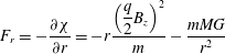 $$\begin{eqnarray}F_{r}=-\frac{\unicode[STIX]{x2202}\unicode[STIX]{x1D712}}{\unicode[STIX]{x2202}r}=-r\frac{\left({\displaystyle \frac{q}{2}}B_{z}\right)^{2}}{m}-\frac{mMG}{r^{2}}\end{eqnarray}$$
and so is inward at all values of
 $r$
which means that the
$r$
which means that the
 $P_{\unicode[STIX]{x1D719}}=0$
particle falls in towards
$P_{\unicode[STIX]{x1D719}}=0$
particle falls in towards
 $r=0$
. The motion is an inward spiral because
$r=0$
. The motion is an inward spiral because
 $P_{\unicode[STIX]{x1D719}}=0$
implies
$P_{\unicode[STIX]{x1D719}}=0$
implies
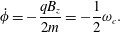 $$\begin{eqnarray}\dot{\unicode[STIX]{x1D719}}=-\frac{qB_{z}}{2m}=-\frac{1}{2}\unicode[STIX]{x1D714}_{c}.\end{eqnarray}$$
Since
 $P_{\unicode[STIX]{x1D719}}$
is a constant of the motion, if a particle initially satisfies (10.12) and so initially has
$P_{\unicode[STIX]{x1D719}}$
is a constant of the motion, if a particle initially satisfies (10.12) and so initially has
 $P_{\unicode[STIX]{x1D719}}=0$
, it will always have
$P_{\unicode[STIX]{x1D719}}=0$
, it will always have
 $P_{\unicode[STIX]{x1D719}}=0$
.
$P_{\unicode[STIX]{x1D719}}=0$
.
A particle that spirals in towards
 $r=0$
thus crosses poloidal flux surfaces and since having
$r=0$
thus crosses poloidal flux surfaces and since having
 $P_{\unicode[STIX]{x1D719}}=0$
is only possible for one sign of particle, only one sign of particle could cross poloidal flux surfaces in the
$P_{\unicode[STIX]{x1D719}}=0$
is only possible for one sign of particle, only one sign of particle could cross poloidal flux surfaces in the
 $z=0$
plane. This would correspond to a radial electric current in the
$z=0$
plane. This would correspond to a radial electric current in the
 $z=0$
plane which is just what is needed to complete the poloidal electric circuit.
$z=0$
plane which is just what is needed to complete the poloidal electric circuit.
Two possible ways for having the required extremely small charge-to-mass ratio are (i) charged dust grains and (ii) very weakly ionized plasma. Charged dust grains were discussed in Bellan (Reference Bellan2008) where it was shown that dust can be charged by various means such as electron impact, photo-ionization, or nuclear processes and typically the equilibrium charge-to-mass ratio of a dust grain is very small compared to that of an electron or ion. Thus, if a dust grain had a charge-to-mass ratio such that at an initial time the dust grain satisfied (10.12) where
 $\dot{\unicode[STIX]{x1D719}}$
is a Kepler angular frequency, the dust grain would spiral in towards
$\dot{\unicode[STIX]{x1D719}}$
is a Kepler angular frequency, the dust grain would spiral in towards
 $r=0$
and so constitute a radial current. While this situation appears possible in principle, it is ‘highly tuned’ as it requires a precise charge-to-mass ratio for at least some dust grains. This situation has been explored in detail in Bellan (Reference Bellan2008).
$r=0$
and so constitute a radial current. While this situation appears possible in principle, it is ‘highly tuned’ as it requires a precise charge-to-mass ratio for at least some dust grains. This situation has been explored in detail in Bellan (Reference Bellan2008).
The situation of a weakly ionized plasma appears more likely because this situation is not highly tuned; this situation was discussed in Bellan (Reference Bellan2016a
, Reference Bellan2017). Here the low charge-to-mass ratio occurs because of collisions between ions and the much larger number of neutrals so that as soon as an ion gains momentum from an electromagnetic force, the ion immediately shares this momentum via collisions with nearby neutrals. If
 $\unicode[STIX]{x1D6FC}$
denotes the ionization fraction, then one ion shares its momentum with
$\unicode[STIX]{x1D6FC}$
denotes the ionization fraction, then one ion shares its momentum with
 $\unicode[STIX]{x1D6FC}^{-1}$
nearby neutrals and so the centre of mass of the ion and the
$\unicode[STIX]{x1D6FC}^{-1}$
nearby neutrals and so the centre of mass of the ion and the
 $\unicode[STIX]{x1D6FC}^{-1}$
neutrals behaves like a particle that has the charge of the ion and the mass of the
$\unicode[STIX]{x1D6FC}^{-1}$
neutrals behaves like a particle that has the charge of the ion and the mass of the
 $\unicode[STIX]{x1D6FC}^{-1}$
neutrals. Thus the centre of mass of a clump consisting of an ion and
$\unicode[STIX]{x1D6FC}^{-1}$
neutrals. Thus the centre of mass of a clump consisting of an ion and
 $\unicode[STIX]{x1D6FC}^{-1}$
neutrals moves like a particle with charge-to-mass ratio given by
$\unicode[STIX]{x1D6FC}^{-1}$
neutrals moves like a particle with charge-to-mass ratio given by
 $\unicode[STIX]{x1D6FC}q/m$
. If, for example, the ionization fraction were
$\unicode[STIX]{x1D6FC}q/m$
. If, for example, the ionization fraction were
 $\unicode[STIX]{x1D6FC}=10^{-12}$
, the cyclotron frequency of the metaparticle represented by the clump would be 12 orders of magnitude smaller than that of an ion and so could easily become comparable to a Kepler frequency. This
$\unicode[STIX]{x1D6FC}=10^{-12}$
, the cyclotron frequency of the metaparticle represented by the clump would be 12 orders of magnitude smaller than that of an ion and so could easily become comparable to a Kepler frequency. This
 $\unicode[STIX]{x1D6FC}^{-1}$
-fold reduction of effective ion cyclotron frequency in a weakly ionized plasma has been previously noted in other contexts by Song, Vasyliunas & Ma (Reference Song, Vasyliunas and Ma2005) and by Pandey & Wardle (Reference Pandey and Wardle2008).
$\unicode[STIX]{x1D6FC}^{-1}$
-fold reduction of effective ion cyclotron frequency in a weakly ionized plasma has been previously noted in other contexts by Song, Vasyliunas & Ma (Reference Song, Vasyliunas and Ma2005) and by Pandey & Wardle (Reference Pandey and Wardle2008).
The ionization fraction in an accretion disk is not uniform but instead is stratified such that
 $\unicode[STIX]{x1D6FC}$
is essentially zero at the accretion disk midplane and then rises to unity at the edge of the accretion disk. This means that all values of
$\unicode[STIX]{x1D6FC}$
is essentially zero at the accretion disk midplane and then rises to unity at the edge of the accretion disk. This means that all values of
 $\unicode[STIX]{x1D6FC}$
from zero to unity exist in the accretion disk and so there will always be some location where
$\unicode[STIX]{x1D6FC}$
from zero to unity exist in the accretion disk and so there will always be some location where
 $\unicode[STIX]{x1D6FC}$
is such that
$\unicode[STIX]{x1D6FC}$
is such that
 $P_{\unicode[STIX]{x1D719}}=0$
for a metaparticle. This metaparticle will spiral inwards and because it contains an ion, the inward spiral corresponds to an inward radial current.
$P_{\unicode[STIX]{x1D719}}=0$
for a metaparticle. This metaparticle will spiral inwards and because it contains an ion, the inward spiral corresponds to an inward radial current.
The inward spiralling metaparticles will accumulate near
 $r=0$
setting up an accumulation of positive charge there. The electrons that originally neutralized the metaparticles cannot spiral in because the electrons do not satisfy
$r=0$
setting up an accumulation of positive charge there. The electrons that originally neutralized the metaparticles cannot spiral in because the electrons do not satisfy
 $P_{\unicode[STIX]{x1D719}}=0$
and so are frozen to poloidal flux surfaces. The electrons can, however, move out of the plane of the accretion disk along poloidal flux surfaces and thus can move by this means towards the origin so as to neutralize the accumulated positive charge. The combined motion of radially inward metaparticles in the accretion disk and electrons moving inward along poloidal flux surfaces in the region exterior to the accretion disk constitute a poloidal electric current having the same topology as in the Caltech jet experiment. This poloidal electric current creates a toroidal magnetic field and the interaction between poloidal current and toroidal magnetic field drives jet motion. This is sketched in figure 17. The combined system thus has accretion (inward moving metaparticles), radial electric current, jets and a mass supply for the jets.
$P_{\unicode[STIX]{x1D719}}=0$
and so are frozen to poloidal flux surfaces. The electrons can, however, move out of the plane of the accretion disk along poloidal flux surfaces and thus can move by this means towards the origin so as to neutralize the accumulated positive charge. The combined motion of radially inward metaparticles in the accretion disk and electrons moving inward along poloidal flux surfaces in the region exterior to the accretion disk constitute a poloidal electric current having the same topology as in the Caltech jet experiment. This poloidal electric current creates a toroidal magnetic field and the interaction between poloidal current and toroidal magnetic field drives jet motion. This is sketched in figure 17. The combined system thus has accretion (inward moving metaparticles), radial electric current, jets and a mass supply for the jets.
The neutralization of the radial electric field by the electrons is only partial and a sufficient radial electric field remains to satisfy the Faraday’s law requirement that the voltage drop associated with this field corresponds to the rate at which toroidal flux is being injected into the jet. The angular momentum of the accreting material is removed by the magnetic force and is done in such a way as to conserve canonical angular momentum.

Figure 17. Poloidal flux surfaces shown as curved black lines. Metaparticles flow radially inwards (horizontal blue arrows) in accretion disk. Electrons outside disk flow along poloidal flux surfaces and produce electric current (blue arrows pointing radially outward and following flux surfaces) that completes poloidal circuit. Accumulation of metaparticles at small radius shown as plus signs and left behind neutralizing electrons shown as minus signs. [Figure from Bellan, Monthly Notices Royal Astronomical Society 458, 4400 (2016).]
Metaparticle behaviour can also be deduced by subtracting the zero mass limit of the electron equation of motion from the MHD equation of motion. It should be noted that by making the substitution
 $\boldsymbol{u}_{e}=\boldsymbol{u}_{i}-\boldsymbol{J}/ne\simeq \boldsymbol{U}-\boldsymbol{J}/ne$
the zero mass limit of the electron equation of motion becomes the generalized Ohm’s law. In the presence of gravity and taking into account the separate contributions to the total pressure from the ions, electrons and neutrals, the MHD equation of motion can be expressed as
$\boldsymbol{u}_{e}=\boldsymbol{u}_{i}-\boldsymbol{J}/ne\simeq \boldsymbol{U}-\boldsymbol{J}/ne$
the zero mass limit of the electron equation of motion becomes the generalized Ohm’s law. In the presence of gravity and taking into account the separate contributions to the total pressure from the ions, electrons and neutrals, the MHD equation of motion can be expressed as
 $$\begin{eqnarray}\unicode[STIX]{x1D70C}\frac{\text{d}\boldsymbol{U}}{\text{d}t}=\boldsymbol{J}\times \boldsymbol{B}-\unicode[STIX]{x1D735}(P_{i}+P_{e}+P_{n})-\unicode[STIX]{x1D70C}\boldsymbol{g}.\end{eqnarray}$$
The electron fluid equation of motion with electron mass neglected is
 $$\begin{eqnarray}0=n_{e}q_{e}(\boldsymbol{E}+\boldsymbol{u}_{e}\times \boldsymbol{B})-\unicode[STIX]{x1D735}P_{e}.\end{eqnarray}$$
Using
 $\boldsymbol{J}=n_{i}q_{i}\boldsymbol{u}_{i}+n_{e}q_{e}\boldsymbol{u}_{e}$
, subtraction of (10.14) from (10.13) gives
$\boldsymbol{J}=n_{i}q_{i}\boldsymbol{u}_{i}+n_{e}q_{e}\boldsymbol{u}_{e}$
, subtraction of (10.14) from (10.13) gives
 $$\begin{eqnarray}\unicode[STIX]{x1D70C}\frac{\text{d}\boldsymbol{U}}{\text{d}t}=-n_{e}q_{e}\boldsymbol{E}+n_{i}q_{i}\boldsymbol{u}_{i}\times \boldsymbol{B}-\unicode[STIX]{x1D735}(P_{i}+P_{n})-\unicode[STIX]{x1D70C}\boldsymbol{g}.\end{eqnarray}$$
Since the plasma is weakly ionized, the overall mass density is essentially the neutral mass density, i.e.
 $\unicode[STIX]{x1D70C}=n_{n}m_{n}$
where
$\unicode[STIX]{x1D70C}=n_{n}m_{n}$
where
 $m_{n}$
and
$m_{n}$
and
 $n_{n}$
are respectively the neutral particle mass and number density. Dividing (10.15) by
$n_{n}$
are respectively the neutral particle mass and number density. Dividing (10.15) by
 $\unicode[STIX]{x1D70C}$
and invoking quasi-neutrality
$\unicode[STIX]{x1D70C}$
and invoking quasi-neutrality
 $n_{e}q_{e}=-n_{i}q_{i}$
gives
$n_{e}q_{e}=-n_{i}q_{i}$
gives
 $$\begin{eqnarray}\frac{\text{d}\boldsymbol{U}}{\text{d}t}=\unicode[STIX]{x1D6FC}\frac{q_{i}}{m_{n}}(\boldsymbol{E}+\boldsymbol{u}_{i}\times \boldsymbol{B})-\frac{\unicode[STIX]{x1D735}(P_{i}+P_{n})}{n_{n}m_{n}}-\boldsymbol{g}.\end{eqnarray}$$
Because the ions collide frequently with the neutrals, the mean ion velocity
 $\boldsymbol{u}_{i}$
is nearly the centre of mass velocity
$\boldsymbol{u}_{i}$
is nearly the centre of mass velocity
 $\boldsymbol{U}$
which is essentially the neutral centre of mass velocity. The ion and centre of mass velocity are presumed to be of order the Kepler velocity which by assumption greatly exceeds thermal velocities. The pressure gradient term scales as
$\boldsymbol{U}$
which is essentially the neutral centre of mass velocity. The ion and centre of mass velocity are presumed to be of order the Kepler velocity which by assumption greatly exceeds thermal velocities. The pressure gradient term scales as
 $v_{T}^{2}/r$
which is much smaller than the centrifugal force
$v_{T}^{2}/r$
which is much smaller than the centrifugal force
 $U_{\unicode[STIX]{x1D719}}^{2}/r$
and so the pressure gradient term can be dropped. Thus, (10.16) reduces to
$U_{\unicode[STIX]{x1D719}}^{2}/r$
and so the pressure gradient term can be dropped. Thus, (10.16) reduces to
 $$\begin{eqnarray}\frac{\text{d}\boldsymbol{U}}{\text{d}t}=\unicode[STIX]{x1D6FC}\frac{q_{i}}{m_{n}}(\boldsymbol{E}+\boldsymbol{U}\times \boldsymbol{B})-\boldsymbol{g},\end{eqnarray}$$
which is the equation of motion of a single particle having charge-to-mass ratio
 $\unicode[STIX]{x1D6FC}q_{i}/m_{n}$
in the presence of electric, magnetic and gravitational fields. Thus, a fluid element of a weakly ionized plasma behaves as a metaparticle and so if the fluid element has
$\unicode[STIX]{x1D6FC}q_{i}/m_{n}$
in the presence of electric, magnetic and gravitational fields. Thus, a fluid element of a weakly ionized plasma behaves as a metaparticle and so if the fluid element has
 $P_{\unicode[STIX]{x1D719}}=0$
, it will spiral in towards the star.
$P_{\unicode[STIX]{x1D719}}=0$
, it will spiral in towards the star.
11 Summary
Because the ideal MHD equations have no intrinsic scale, they apply over an enormous range all the way from laboratory experiments to non-relativistic astrophysical jets. Although not in equilibrium because unbalanced forces provide acceleration, jets can be considered to be in a quasi-steady state. Analysis of jets requires subdividing the jet into different regions as the physics of these regions differ.
The launching region has an applied electromotive force that injects toroidal magnetic flux, a mass source and frozen-in poloidal flux. The main column is highly collimated, has approximate radial force balance and a modified Bernoulli relation in the axial direction. The jet tip has a retarding force associated with the splaying out and axial bunching of the poloidal field lines near the tip. This retarding force causes a bunching up of the axial flow near the tip and this axial compression squeezes the frozen-in toroidal flux so as to increase the toroidal magnetic field. This increase corresponds to increasing the pinch force and so the jet continuously collimates at the tip as it propagates.
Jets become susceptible to the kink instability on reaching a critical length and, at least in laboratory experiments, the effective gravity from the lateral acceleration of the kink instability provides the setting for a Rayleigh–Taylor secondary instability. The Rayleigh–Taylor instability can choke the current flowing in the jet and cause the jet to break. Jets become compressed when they impact a target cloud.
Ideal MHD is inadequate to describe the launching region because magnetic flux must be injected into the plasma in this region whereas ideal MHD requires the magnetic flux in the plasma frame to be unchanging. However, by including Hall terms in the Ohm’s law, flux is no longer frozen in and so can be injected. In order to have a complete path for the electric current flowing in a jet, the current must flow across poloidal flux surfaces but this is forbidden in ideal MHD because charged particles cannot move continuously across poloidal flux surfaces as would be required for a continuous electric current across flux surfaces.
If the particle charge-to-mass ratio is orders of magnitude smaller than that of an ion or electron, a particle effectively develops such a large orbit that it is no longer frozen to poloidal flux surfaces. This extremely small charge-to-mass ratio is feasible for charged dust grains and an equivalent situation occurs when the plasma is very weakly ionized and highly collisional. In this latter case, each ion is effectively bound to a large number of neutrals so the combination of the ion and its bound neutrals moves like a metaparticle having a very small charge-to-mass ratio. Particles with a critical small charge-to-mass ratio spiral in towards the star and this motion provides the electric current needed to complete the circuit of the poloidal electric current flowing from the disk to the jet and back to the disk. This poloidal electric current creates the toroidal magnetic field the gradient of which is responsible for driving the jet.
Acknowledgements
This material is based upon work supported by the US Department of Energy Office of Science, Office of Fusion Energy Sciences under award no. DE-FG02-04ER54755 as part of the NSF/DOE Partnership in Plasma Science. The data in figure 13 come from work supported by the US Department of Energy Advance Research Projects Agency – Energy under award no. DE-AR0000565.
Appendix A. Relation to other experiments
The Imperial College
 $Z$
-pinch experiment (Lebedev et al.
Reference Lebedev, Ciardi, Ampleford, Bland, Bott, Chittenden, Hall, Rapley, Jennings and Sherlock2005) differs from the experiment described here in that the Imperial College experiment has no poloidal magnetic field and is surrounded by a cocoon of high-pressure gas. The Imperial College experiment was described as a magnetic tower which is consistent with having a cocoon of high-pressure gas but appears to be at variance with the force-free assumption intrinsic to the magnetic tower model. This is because a force-free magnetic field implies existence of both toroidal and poloidal field components to give
$Z$
-pinch experiment (Lebedev et al.
Reference Lebedev, Ciardi, Ampleford, Bland, Bott, Chittenden, Hall, Rapley, Jennings and Sherlock2005) differs from the experiment described here in that the Imperial College experiment has no poloidal magnetic field and is surrounded by a cocoon of high-pressure gas. The Imperial College experiment was described as a magnetic tower which is consistent with having a cocoon of high-pressure gas but appears to be at variance with the force-free assumption intrinsic to the magnetic tower model. This is because a force-free magnetic field implies existence of both toroidal and poloidal field components to give
 $\unicode[STIX]{x1D735}\times \boldsymbol{B}=\unicode[STIX]{x1D706}\boldsymbol{B}$
. An important feature of the Imperial College
$\unicode[STIX]{x1D735}\times \boldsymbol{B}=\unicode[STIX]{x1D706}\boldsymbol{B}$
. An important feature of the Imperial College
 $Z$
-pinch was the observation by Suzuki-Vidal et al. (Reference Suzuki-Vidal, Lebedev, Bland, Hall, Swadling, Harvey-Thompson, Chittenden, Marocchino, Ciardi and Frank2010) of episodic behaviour where the jet velocity was modulated by instabilities at the source with the result that faster jet segments would catch up with slower segments and create shocks.
$Z$
-pinch was the observation by Suzuki-Vidal et al. (Reference Suzuki-Vidal, Lebedev, Bland, Hall, Swadling, Harvey-Thompson, Chittenden, Marocchino, Ciardi and Frank2010) of episodic behaviour where the jet velocity was modulated by instabilities at the source with the result that faster jet segments would catch up with slower segments and create shocks.
The LULI laser experiment (Abertazzi et al.
Reference Abertazzi, Ciardi, Nakatsutsumi, Vinci, Beard, Bonito, Billette, Borghesi, Burkley and Chen2014) had a strong externally imposed homogeneous poloidal magnetic field (
 $z$
direction) that had dimensions much larger than the plasma jet so the observed collimation was essentially the plasma flowing along this imposed axial magnetic field. Also, rather than having peak density on axis, the axis region was observed to be a cavity with density peaking somewhat off axis. Axial plasma flow at the rim of the cavity was observed to focus at the jet tip and form a shock that heated the plasma. The LULI experiment is thus quite different from the Caltech experiment because the LULI experiment does not have an axial stretching of poloidal magnetic field by the pressure of toroidal magnetic field as was sketched in figure 1. Also, although self-generated toroidal magnetic fields are presumed to exist, they are claimed to have negligible effect and so the jet velocity is entirely from the hydrodynamic pressure gradient established by the laser pulse. Thus, the LULI experiment has no MHD acceleration of the jet and no MHD confinement, only a channelling of a hydrodynamic flow by an imposed axial magnetic field.
$z$
direction) that had dimensions much larger than the plasma jet so the observed collimation was essentially the plasma flowing along this imposed axial magnetic field. Also, rather than having peak density on axis, the axis region was observed to be a cavity with density peaking somewhat off axis. Axial plasma flow at the rim of the cavity was observed to focus at the jet tip and form a shock that heated the plasma. The LULI experiment is thus quite different from the Caltech experiment because the LULI experiment does not have an axial stretching of poloidal magnetic field by the pressure of toroidal magnetic field as was sketched in figure 1. Also, although self-generated toroidal magnetic fields are presumed to exist, they are claimed to have negligible effect and so the jet velocity is entirely from the hydrodynamic pressure gradient established by the laser pulse. Thus, the LULI experiment has no MHD acceleration of the jet and no MHD confinement, only a channelling of a hydrodynamic flow by an imposed axial magnetic field.
The University of Rochester experiment (Li et al.
Reference Li, Tzeferacos, Lamb, Gregori, Norreys, Rosenberg, Follett, Froula, Koenig and Seguin2016) does not have an externally imposed magnetic field but instead has self-generated magnetic fields produced by the Biermann battery effect, i.e.
 $\unicode[STIX]{x2202}\boldsymbol{B}/\unicode[STIX]{x2202}t\sim \unicode[STIX]{x1D735}n\times \unicode[STIX]{x1D735}T$
. It is argued that two field structures created by this effect merge and then, by means of reconnection, form a field that can be decomposed into toroidal and poloidal components. The jet is assumed to be thermally launched rather than magnetically accelerated but is also assumed to carry frozen-in toroidal and poloidal magnetic fields. Periodic structures observed by proton radiography are interpreted as kink instabilities. This interpretation is made because the embedded toroidal magnetic field is presumed to be strong relative to the embedded poloidal magnetic field so that the Kruskal–Shafranov kink threshold is exceeded.
$\unicode[STIX]{x2202}\boldsymbol{B}/\unicode[STIX]{x2202}t\sim \unicode[STIX]{x1D735}n\times \unicode[STIX]{x1D735}T$
. It is argued that two field structures created by this effect merge and then, by means of reconnection, form a field that can be decomposed into toroidal and poloidal components. The jet is assumed to be thermally launched rather than magnetically accelerated but is also assumed to carry frozen-in toroidal and poloidal magnetic fields. Periodic structures observed by proton radiography are interpreted as kink instabilities. This interpretation is made because the embedded toroidal magnetic field is presumed to be strong relative to the embedded poloidal magnetic field so that the Kruskal–Shafranov kink threshold is exceeded.
Some relative properties of the Caltech, Imperial College, LULI and University of Rochester experiments are summarized in table 1. The cost per shot in the Caltech experiment is negligible because nothing is destroyed during a shot so another shot can be made within about two minutes; this allows scans of parameters over many shots to determine measurements of parametric dependence as for example was shown in figure 7 or for the threshold of the kink instability as was reported in Hsu & Bellan (Reference Hsu and Bellan2003). The Imperial College, LULI, and University of Rochester experiments involve destruction of the structure creating the jet and also destruction of portions of the diagnostics. This means that the structures creating the jet and parts of the diagnostics need to be replaced after each shot; this greatly constrains the number of shots so that interpretation of the experiments is mainly done by comparison of one or a few shots to numerical models. In contrast, it is possible in the Caltech experiment to scan parameters or move a probe over many shots to establish an experimentally measured scaling or an experimentally determined spatial profile. The time-dependent interior magnetic field profile of the Caltech experiment has been measured directly by magnetic probes and these measurements have been confirmed by spectroscopic measurement of Zeeman line splitting (Shikama & Bellan Reference Shikama and Bellan2013). The interior magnetic field profile in the Imperial College experiment has been estimated using comparisons with computer models; a single-point magnetic probe measurement has been made but the calibration was uncertain (Suzuki-Vidal et al.
Reference Suzuki-Vidal, Lebedev, Ciardi, Bland, Hall, Swadling, Harvey-Thompson, Burdiak, Grouchy and Chittenden2014). The interior magnetic field in the LULI experiment is imposed by an external solenoid and is presumed to be straight. The interior magnetic field in the University of Rochester experiment has been determined indirectly by applying a model of caustics to proton radiography images. The
 $Z$
-pinch and laser plasmas have magnetic fields, plasma densities and plasma temperatures that are several orders of magnitude larger than in the Caltech plasma.
$Z$
-pinch and laser plasmas have magnetic fields, plasma densities and plasma temperatures that are several orders of magnitude larger than in the Caltech plasma.
Table 1. Comparison of relative properties of different jet experiments. The poloidal field in the Caltech experiment is produced by an external coil and the toroidal field from an electric current flowing from electrodes. The toroidal field in the Imperial College experiments also comes from an electric current flowing from electrodes. The poloidal field in the LULI experiment comes from a pair of coils that are far from the plasma. The poloidal and toroidal fields in the University of Rochester experiment are assumed to be produced by the merging of currents produced by the Biermann battery mechanism.