


1 Introduction
Ultra-intense lasers (Danson et al. Reference Danson, Haefner, Bromage, Butcher, Chanteloup, Chowdhury, Galvanauskas, Gizzi, Hein and Hillier2019) have been used for more than two decades to produce neutrons (Pretzler et al. Reference Pretzler, Saemann, Pukhov, Rudolph, Schätz, Schramm, Thirolf, Habs, Eidmann, Tsakiris, Meyer-ter Vehn and Witte1998; Disdier et al. Reference Disdier, Garçonnet, Malka and Miquel1999) with fewer radiological constraints than conventional neutron sources, such as reactors or accelerator-based spallation sources. Indeed, the former produce large quantities of radioactive waste due to the fission reactions and the significant activation of their constituent materials (Bungau et al. Reference Bungau, Bungau, Cywinski, Barlow, Robert Edgecock, Carlsson, Danared, Mezei, Ivalu Sander Holm, Pape Møller and Dølrath Thomsen2014; IAEA 2022). Laser-driven neutron sources are characterized by significant emission of neutrons, from sub-MeV to tens or hundreds of MeV, in small time intervals (less than nanoseconds) leading to high-brightness short neutron pulses (Lancaster et al. Reference Lancaster, Karsch, Habara, Beg, Clark, Freeman, Key, King, Kodama, Krushelnick, Ledingham, McKenna, Murphy, Norreys, Stephens, Stöeckl, Toyama, Wei and Zepf2004; Alvarez et al. Reference Alvarez, Fernández-Tobias, Mima, Nakai, Kar, Kato and Perlado2014; Higginson et al. Reference Higginson, Vassura, Gugiu, Antici, Borghesi, Brauckmann, Diouf, Green, Palumbo, Petrascu, Sofia, Stardubtsev, Willi, Kar, Negoita and Fuchs2015; Alejo et al. Reference Alejo, Ahmed, Green, Mirfayzi, Borghesi and Kar2016; Hornỳ et al. Reference Hornỳ, Chen, Davoine, Lelasseux, Gremillet and Fuchs2022). These features are of potential interest for many applications in astrophysics (Guerrero et al. Reference Guerrero, Domingo-Pardo, Kaeppeler, Lerendegui-Marco, Palomo, Quesada and Reifarth2017; Chen et al. Reference Chen, Negoita, Spohr, d'Humières, Pomerantz and Fuchs2019), plasma physics (Higginson et al. Reference Higginson, McNaney, Swift, Bartal, Hey, Kodama, Le Pape, Mackinnon, Mariscal, Nakamura, Nakanii, Tanaka and Beg2010; Fernández et al. Reference Fernández, Barnes, Mocko and Zavorka2019), medical sciences (Franchet-Beuzit et al. Reference Franchet-Beuzit, Spotheim-Maurizot, Sabattier, Blazy-Baudras and Charlier1993; Wittig et al. Reference Wittig, Michel, Moss, Stecher-Rasmussen, Arlinghaus, Bendel, Luigi Mauri, Altieri, Hilger, Salvadori, Menichetti, Zamenhof and Sauerwein2008), security (Buffler Reference Buffler2004; Martz & Glenn Reference Martz and Glenn2022), industry (Takenaka et al. Reference Takenaka, Asano, Fujii, Mizubata and Yoshii1999) or non-destructive material analysis (Gratuze et al. Reference Gratuze, Barrandon, Dulin and Al Isa1992; Noguere et al. Reference Noguere, Cserpak, Ingelbrecht, Plompen, Quetel and Schillebeeckx2007).
Several mechanisms can be used to produce neutrons using lasers, among them: photoneutron generation (Pomerantz et al. Reference Pomerantz, McCary, Meadows, Arefiev, Bernstein, Chester, Cortez, Donovan, Dyer, Gaul, Hamilton, Kuk, Lestrade, Wang, Ditmire and Hegelich2014), beam-fusion reactions (Ditmire et al. Reference Ditmire, Zweiback, Yanovsky, Cowan, Hays and Wharton1999; Mirfayzi et al. Reference Mirfayzi, Kar, Ahmed, Krygier, Green, Alejo, Clarke, Freeman, Fuchs, Jung, Kleinschmidt, Morrison, Najmudin, Nakamura, Norreys, Oliver, Roth, Vassura, Zepf and Borghesi2015) or the pitcher–catcher technique. The principle of the pitcher–catcher technique has been widely demonstrated (Lancaster et al. Reference Lancaster, Karsch, Habara, Beg, Clark, Freeman, Key, King, Kodama, Krushelnick, Ledingham, McKenna, Murphy, Norreys, Stephens, Stöeckl, Toyama, Wei and Zepf2004; Higginson et al. Reference Higginson, McNaney, Swift, Petrov, Davis, Frenje, Jarrott, Kodama, Lancaster, Mackinnon, Nakamura, Patel, Tynan and Beg2011; Roth et al. Reference Roth2013; Storm et al. Reference Storm, Jiang, Wertepny, Orban, Morrison, Willis, McCary, Belancourt, Snyder, Chowdhury, Bang, Gaul, Dyer, Ditmire, Freeman and Akli2013; Kleinschmidt et al. Reference Kleinschmidt, Bagnoud, Deppert, Favalli, Frydrych, Hornung, Jahn, Schaumann, Tebartz, Wagner, Wurden, Zielbauer and Roth2018). It allows for the generation of neutrons via the interaction of laser-accelerated ions (usually protons) with a second target called the converter. The selection of this converter depends on the proton energy distribution. A low-$Z$ material (like Li or Be) should be selected if the proton spectrum is peaked at energies of a few MeV, to take advantage of the cross-sections of (p,n) reactions at these energies. However, a high-$Z$
 material is preferred if the proton spectrum has a larger component at energies of tens of MeV, so as to benefit from spallation reactions (Martinez et al. Reference Martinez, Chen, Bolaños, Blanchot, Boutoux, Cayzac, Courtois, Davoine, Duval, Horny, Lantuejoul, Le Deroff, Masson-Laborde, Sary, Vauzour, Smets, Gremillet and Fuchs2022).
The laser acceleration of ions is itself induced by laser-generated hot electrons that form a dense sheath on the solid target irradiated by the laser; this is the so-called target normal sheath acceleration (TNSA) mechanism (Snavely et al. Reference Snavely, Key, Hatchett, Cowan, Roth, Phillips, Stoyer, Henry, Sangster, Singh, Wilks, MacKinnon, Offenberger, Pennington, Yasuike, Langdon, Lasinski, Johnson, Perry and Campbell2000; Wilks et al. Reference Wilks, Langdon, Cowan, Roth, Singh, Hatchett, Key, Pennington, MacKinnon and Snavely2001; Macchi, Borghesi & Passoni Reference Macchi, Borghesi and Passoni2013; Poole et al. Reference Poole, Obst, Cochran, Metzkes, Schlenvoigt, Prencipe, Kluge, Cowan, Schramm, Schumacher and Zeil2018).
We present here the results of an experiment carried out using the Titan laser and aimed at performing a global characterization of laser-driven neutrons. The neutrons were produced by the interaction of protons, accelerated from plastic targets, with a LiF converter. The neutron emissions were characterized using a set of diagnostics, including organic plastic scintillators used as neutron time-of-flight (nToF) detectors, CR-39 and activation foils, and also simulated with Monte Carlo transport codes MCNP6 (Thompson Reference Thompson1979) and Geant4 (Agostinelli et al. Reference Agostinelli2003).
Section 2 gives an overview of the experimental set-up and the characteristics of the proton spectrum used to produce neutrons. Section 3 describes how the neutron emissions were simulated using a Monte Carlo code. Section 4 shows the experimental measurements obtained using the different diagnostics and § 5 presents comparisons with the simulated results. Finally, § 6 summarizes the main results and concludes this study.
2 Experimental overview
2.1 Experimental set-up
The experiment was performed using the Titan laser at the Jupiter Laser Facility at Lawrence Livermore National Laboratory, delivering pulses with 1054 nm wavelength and 650 fs duration. The laser was focused using an $f/3$ off-axis parabola to achieve an 8 $\mathrm {\mu }$
 m full-width-at-half-maximum focal spot. With an on-target energy of ${\sim }100\ {\rm J}$
 , the on-target peak intensity was around $10^{20}\ {\rm W}\ {\rm cm}^{-2}$
 .
.
As shown in figure 1, the beam was focused onto a 23 $\mathrm {\mu }$ m polyethylene terephthalate (PET) target that was aluminized with a few micrometres on the target surface to increase laser absorption. The laser-accelerated protons emanated from the rear surface of the target using the TNSA mechanism. These protons were aimed into a 2 mm thick LiF slab placed 20 mm away, where they caused the generation of neutrons via nuclear reactions:


Figure 1. Scheme of the diagnostic set-up for the activation measurements, where the activation stack was placed at its closest distance to the LiF (shot 42). In the other set-up, the stack was placed further back such that $L = 205$ mm (shot 25).
The neutrons were characterized with a variety of diagnostics to measure their yield, such as CR-39, neutron activation of various isotopes (i.e. $^{115}\textrm {In}$ , $^{27}\textrm {Al}$
 , $^{56}\textrm {Fe}$
 ) and a direct measurement of the neutron generation by measuring the amount of residual Be activity produced in the LiF slab.
The energy and angular dependence of the neutron yields were also experimentally studied using organic plastic scintillators (BC-400) for nToF measurements. As shown in figure 2, a number of BC-400 scintillators with dimensions of $4\times 4\times 12\ \textrm {cm}^{3}$ were placed at different angles and distances between 2 and 6 ms relative to the proton beam direction and secondary LiF target, respectively. The photomultiplier tube used was a Photonis XP2972 and its outputs were digitized for a duration of 1 $\mathrm {\mu }$
 s at 1GS/s rate using a V1743 multichannel 12 bits switch-capacitor digitizer from CAEN.

Figure 2. Arrangement of the nToF detectors and their configurations of Pb shielding in the experimental hall.
2.2 Proton spectrum
The proton spectrum was measured using layers of Gafchromic HD Radiochromic Film (RCF) (Nürnberg et al. Reference Nürnberg, Schollmeier, Brambrink, Blažević, Carroll, Flippo, Gautier, Geißel, Harres, Hegelich, Lundh, Markey, McKenna, Neely, Schreiber and Roth2009) separated by filters of PET placed at 35 mm behind the target, in place of the LiF converter. The dose deposition was modelled using stopping powers taken from SRIM (Ziegler Reference Ziegler2004). As shown in figure 3, the proton spectrum, $({\textrm {d}N_{p}}/{\textrm {d}E}) (E_{p})$ , was fitted using an exponential spectrum:


where $E_{p}$ is the proton energy, $N_{0}$
 is the total number of protons, $T$
 is the slope temperature and $E_{\max } = 30.5$
 MeV is the cut-off or maximum proton energy, set by the last layer of RCF with visible signal.

Figure 3. Measured proton energy spectrum. The circles show the proton spectrum inferred using RCF and the dashed line is a decaying exponential, with parameters $N_{0} = 2.14\times 10^{12}$ , $T = 6.3$
 MeV and $E_{\max } = 30.5$
 MeV. The solid background shows the region of calculated uncertainty within one standard deviation of $1.3\times 10^{11}$
 for $N_{0}$
 and 0.2 MeV for $T$
 .
.
The fitting was performed by minimizing the reduced chi-squared value:

where $N$ is the number of fitting points, $m=2$
 is the number of fitting parameters, $y_{i}$
 is the experimental data, $f$
 is the exponential fit and $\sigma _{i}$
 is the uncertainty in the RCF data. The best fit to the data was found with $N_{0} = 2.14\times 10^{12}$
 and $T = 6.3$
 MeV, giving $\chi _{\nu }^{2} = 2.97$
 . The uncertainty in the fitting parameters was $1.3\times 10^{11}$
 for $N_{0}$
 and 0.2 MeV for $T$
 .
.
3 Monte Carlo modelling of neutron production
To simulate the production of neutrons in the LiF slab, the Monte Carlo code Geant4 was used. This code includes particle scattering, energy loss and nuclear reactions. The proton-induced nuclear reactions included were $^7\textrm {Li(p,n)}^7\textrm {Be}$ , $^6\textrm {Li(p,n)}^6\textrm {Be}$
 and $^{19}\textrm {F(p,n)}^{19}\textrm {Ne}$
 , with cross-sections taken from the ENDF/B-VIII.O library (Brown et al. Reference Brown, Chadwick, Capote, Kahler, Trkov, Herman, Sonzogni, Danon, Carlson and Dunn2018), which contains information on the angular dependence of these cross-sections. As an example, the $^7\textrm {Li(p,n)}^7\textrm {Be}$
 cross-section obtained from ENDF/B-VIII.O is shown in figure 4.

Figure 4. Cross-section used for simulating the $^7\textrm {Li(p,n)}^7\textrm {Be}$ reaction.
The protons were injected in the simulation into a LiF target at a distance of 1 mm and allowed to propagate through a 2 mm thick LiF target (as in the experiment). The protons were given an exponential energy spectrum as described in § 2.2. They were injected at the centre of the LiF, which is a simplification because the proton beam should have a diameter of approximately 20 mm in the experiment due the divergence of the beam. The protons were injected with straight trajectories, which is another simplification as the proton beam will have a divergence angle. Note that the measurements of the proton spectrum shown in figure 3 and the neutron conversion in the LiF converter were performed in different shots. Due to the shot-to-shot variability of the laser parameters, the real proton spectrum injected in the converter to produce the neutrons could differ from the one provided in figure 3. An example of the shot-to-shot variability is shown in figure 3 of Higginson et al. (Reference Higginson, McNaney, Swift, Bartal, Hey, Kodama, Le Pape, Mackinnon, Mariscal, Nakamura, Nakanii, Tanaka and Beg2010) using the same laser with similar conditions.
Spherical detectors were placed in the simulations at angles of 0$^\circ$ , 45$^\circ$
 , 90$^\circ$
 , 135$^\circ$
 and 180$^\circ$
 with respect to the injected protons, as shown in figure 5. These detectors were approximately 40 mm away from the front surface of the LiF and had diameters of 25 mm. Neutrons passing through these detectors were binned in energy and normalized by the solid angle of the detectors.

Figure 5. Schematic of the set-up used for the Geant4 simulations. The arrow shows the direction of the proton injection. The detection spheres are shown as circles.
Figure 6 shows the simulated yields of the detectors resolved in angle. For the injected proton spectrum, the neutron yield is relatively flat as a function of angle, as varying only by about a factor of 2.5. Inclusion of the divergence angle of the protons would result in a more isotropic distribution. The expected divergence is 30$^\circ$ [7] which we would expect to moderately smooth the angular yield.

Figure 6. The neutron yields (a) and neutron spectra (b) at different angles as found from Geant4 simulations.
Figure 6 shows the energy spectra of the neutrons in the different detectors. The peak in the cross-section which starts at around 4 MeV at 0$^\circ$ moves to lower energies as the angle increases, which is due to the kinematics of the interaction. Also, the higher-energy neutrons are more likely to be observed at forward-directed angles. Again, including the proton angular divergence would minimize these effects.
These neutron spectra will next be used to model the responses of the diagnostics. The total number of neutrons recorded in these simulations was $9.80\times 10^{8}$ neutrons. Additional simulations were run to obtain the number of neutrons produced only from Li. This number was found to be $8.92\times 10^{8}$
 , which can be compared with the activation found via measurement of the $^7\textrm {Be}$
 decay as shown in table 1.
Table 1. Experimental measurement of activity and number, $N$ , of $^7\textrm {Be}$
 nuclei residuals from the $^7\textrm {Li(p,n)}^7\textrm {Be}$
 reaction in the LiF slab.

4 Neutron yield diagnostics
4.1 Activation measurements
4.1.1 Set-up and characteristics of activation measurements
The activation samples were counted at two locations using high-purity Ge detectors. The first location was onsite at the Titan laser, and the second was at the Lawrence Livermore National Laboratory's Nuclear Counting Facility (NCF). The NCF is a low-background facility located underground, beneath six feet of magnetite, housing a dozen high-purity Ge detectors each surrounded by 10 cm of pre-World War II lead to minimize contributions from environmental radiation. A customized program, GAMANAL, performs background subtractions and peak fits, correcting for individual detector efficiency, sample geometry and self-shielding of gamma-rays in the samples (Gunnink & Niday Reference Gunnink and Niday1972). The detectors are regularly calibrated against NIST-traceable multi-energy point sources and large-area distributed sources. Automated sample positioning systems ensure accurate and repeatable counting geometries. At the onsite location, Ge detector absolute efficiencies were calculated to take into account the various geometries of the irradiated samples.
Gamma decays at 844, 847 and 336 keV were used to measure neutron activation yields in samples of Al, Fe and In, respectively. The number of neutrons produced in the $^7\textrm {Li(p,n)}$ reaction were measured using the $^7\textrm {Li}$
 478 keV gamma line populated in the electron capture decay of the $^7\textrm {Be}$
 ground state (Kinsey et al. 2008). At the end of each laser shot, the total number of radioactive nuclei present in the samples were deduced from the number of decays measured during time intervals starting at the time after the laser shot. The branching ratios of each transition were taken into account.
4.1.2 Neutron characterization via residuals in LiF
The direct measurement of the total neutron production is the measurement of the residual isotopes in the LiF (i.e. the product) following irradiation. The nuclear reactions that generate neutrons from the proton reactions are $^7\textrm {Li(p,n)}^7\textrm {Be}$ , $^6\textrm {Li(p,n)}^6\textrm {Be}$
 and $^{19}\textrm {F(p,n)}^{19}\textrm {Ne}$
 , as shown at the top of table 2. Unfortunately, the half-lives of both $^6\textrm {Be}$
 and $^{19}\textrm {Ne}$
 are under 20 s and thus too fast to make measurements feasible ex situ due the time (${\sim }10$
 minutes) needed to vent the chamber, though such measurements might be possible via in situ counting in the future. However, the $^7\textrm {Be}$
 residual has a half-life of 53.2 days and a gamma decay energy of 478 keV, which is easily measured outside of the chamber. Figure 7 shows the onsite high-purity Ge energy spectra of the LiF residual decay from shot 42. The measured activities are given in table 1.
Table 2. List of candidates for residual and neutron activation measurements. The columns show, in order, the initial isotope, its abundance, the reaction type, the reaction threshold, the residual isotope, its half-life and the gamma-decay energy detected via spectroscopy. The final three columns show the estimated total number of residuals, the activity at time zero and the activity 20 minutes after the shot. These estimates come from the Monte Carlo simulations detailed in § 3. Note that, as detailed in the main text, the estimates of the neutron activation measurements are made considering a 25 mm diameter sample, of 10 mm thickness, placed 40 mm from the target. This is not the exact experimental set-up, but it aided in designing the activation stack used in the experiment.
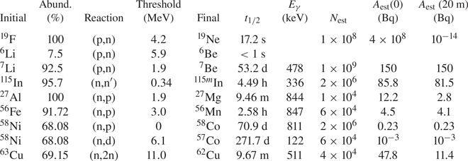

Figure 7. Activation spectra of the LiF using the onsite high-purity Ge. The 478 and 511 keV lines are from the $^7\textrm {Be}$ decay and electron–positron annihilation, respectively.
To estimate the number of residual isotopes and their activity, we used Monte Carlo simulations (detailed in § 3), which include the $^7\textrm {Li(p,n)}^7\textrm {Be}$ reaction. These yield a total number of residuals of $8.92\times 10^{8}$
 and an activity of 134 Bq. Table 1 shows the activation measured from the decay of $^7\textrm {Be}$
 residuals. The $^7\textrm {Be}$
 decay was measured both onsite and at the NCF on shot 42. The latter provided a slightly lower yield relative to that measured using the onsite detectors by a factor of 0.93. Given the high fidelity of NCF, this was considered a correction factor for the onsite data. Shot 25 only had onsite data and was corrected by this factor.
From table 2, we observe that our simulations predict a total number of neutrons by, on average, a factor of 2 times lower than the neutrons observed experimentally. The origin of this difference could lie in the shot-to-shot variation of the proton spectrum, as discussed in § 3.
4.1.3 Neutron characterization via activation samples
Additionally, a stack of activation foils with multiple materials, illustrated in figure 1, was used to infer the neutron yields and, due to the energy dependence of the cross-sections, some energy resolution (Stoulos et al. Reference Stoulos, Koseoglou, Vagena and Manolopoulou2016).
For this experiment, we investigated multiple neutron activation materials, as listed in table 2, to determine the best ones to use for this particular experiment. For this evaluation, we use the neutron spectrum calculated in § 3, and estimated the reactions, using the Monte Carlo code MCNP, in a cylindrical puck of 25 mm diameter, 10 mm thickness, placed 40 mm away from the LiF.
These were not the final sizes used in the experiment (i.e. they are different from those of figure 1), but they help to compare the different materials and are consistent with the geometries required to fit inside the chamber and allow for measurements at multiple angles. The results of these estimations are listed in table 2.
Figure 8 shows the cross-sections of the materials considered for this neutron activation diagnosis as taken from the TENDL library (Koning et al. Reference Koning, Rochman, Sublet, Dzysiuk, Fleming and Van der Marck2019).

Figure 8. Cross-sections for neutron-induced reactions of interest for activation analysis.
Based on these estimates, some of the activation materials were excluded from the experiment. For example, both of the reactions in $^{58}\textrm {Ni}$ were excluded due to the very low activity, which stems not from the number of activations, but from the very long half-life of the products. The copper sample was excluded, not due to the low activity, but to the fact that the copious gamma-rays produced in the laser interaction may create activity in the sample via the $^{63}\textrm {Cu}(\gamma,\textrm {n})^{62}\textrm {Cu}$
 or $^{65}\textrm {Cu}(\gamma,\textrm {n})^{64}\textrm {Cu}$
 reactions, which produce products indistinguishable from those of the neutron-generated reactions: $^{63}\textrm {Cu}(\textrm {n,2n})^{62}\textrm {Cu}$
 and $^{65}\textrm {Cu}(\textrm {n,2n})^{64}\textrm {Cu}$
 , respectively.
The materials that were chosen for this experiment were thus Al, Fe and In, which were used in their natural abundances. Figure 1 shows the activation pack, which consisted of, in order of proximity to the LiF neutron source, an indium cylindrical puck ($\textrm {thickness} = 3$ mm, $\textrm {diameter} = 25$
 mm, $\rho = 7.31$
 g cm$^{-3}$
 ), a steel slab, which we approximate as iron ($\textrm {thickness} = 12.5$
 mm, $\textrm {area} = 20 \times 30\ \textrm {mm}^{2}$
 , $\rho = 7.87$
 g cm$^{-3}$
 ), an aluminium cylindrical puck ($\textrm {thickness} = 10$
 mm, $\textrm {diameter} = 25$
 mm, $\rho = 2.69$
 g cm$^{-3}$
 ) and followed by the CR-39, which is explained in § 4.3.
This stack was placed at 0$^\circ$ from the direction of the proton propagation and at either 45 or 205 mm from the front of the indium to the LiF. The solid angle, $\varOmega$
 , was calculated as a function of the angle $\varTheta$
 subtended by the activation sample with radius $R$
 and distance $D$
 from the source:

In the case of the square-shaped iron, an effective radius of $R^{2} = S/{\rm \pi}$ was used, where $S$
 is the surface of the detector piece. The results from these measurements are shown in table 3.
Table 3. Measured activities at shot time, $A(0)$ , the corresponding number of nuclei, $N$
 , and the number of nuclei per solid angle, $\textrm {d}N/\textrm {d}\varOmega$
 .
.

4.2 Neutron time-of-flight diagnostics
4.2.1 Simulation of the nToF response
To analyse the experimental nToF signals, simulations were performed using the Geant4 toolkit, as it allowed for modelling the scintillation processes in the detectors. The simulated neutron energy distributions of figure 6 were used as an input for Geant4. The experimental set-up and the interactions of the neutrons in the experimental hall were simulated and nToF temporal distributions were obtained.
The simulations included the Al interaction chamber, the concrete walls of the experimental hall with a thickness of 40 cm and the Pb configurations shielding each of the detectors. The response of the BC-400 scintillators in terms of scintillation photon yield was set according to Saint-Gobain Crystals (2015) and Verbinski et al. (Reference Verbinski, Burrus, Love, Zobel, Hill and Textor1968) and the neutron interactions were simulated using the QGSP_BIC_HP physics list. The simulated nToF distributions were convolved with a Gaussian with a full width at half-maximum of 10 ns that is the measured detector response to a single interaction.
The effects of the different components of the experimental set-up on the nToF signals were studied through simulations. Figure 9 presents the simulated nToF signals, under different configurations, for Detector 10 (placed at 191$^\circ$ and 5.14 m from the target; see figure 2). The distributions in the figure are normalized to each other according to the total number of events registered with the detector.

Figure 9. Effects of the addition of different volumes in the simulations of the nToF signals for Detector 10.
The changes in the shape of the nToF signals are clearly observed as more of the environmental surroundings are added to the simulated configuration. The scattering effect can also be visualized in a two-dimensional graph where the relation between the time of flight for the detected event and the initial neutron energy is plotted. Such a plot for Detector 10 in the full configuration simulation is presented in figure 10. The points correspond to events in the detector and it is clearly visible that wide ranges of time-of-flight values correspond to neutrons with the same initial energy.

Figure 10. Relationship between the simulated time-of-flight distribution and the initial energy of the neutrons, for Detector 10, with a 30 cm thick front Pb shielding.
4.2.2 The nToF measurements
The response of the detector was the result of neutron and X-ray/gamma-ray interactions with the scintillator. However, since the X-rays/gamma-rays travel at the speed of light, whereas the neutrons are much slower, there is a temporal separation between the two induced signals, as can be seen in figure 11. A shielding comprising several Pb bricks was placed around each detector to reduce the saturation effects due to the strong hard X-ray flash associated with the laser interaction with the (primary) target (Ditmire et al. Reference Ditmire, Zweiback, Yanovsky, Cowan, Hays and Wharton1999; Jung et al. Reference Kinsey2013). The thickness of the Pb shielding in the direction of the Al interaction chamber was in the range of 20 to 40 cm for the different detectors. The arrangement of the scintillators and their shielding is presented in figure 2.

Figure 11. Background subtraction procedure in the experiment for Detector 10, with a 30 cm thick front Pb shielding: (black) nToF for the detector in the shot of interest after the $\gamma$ -peak time alignment; (red) background distribution from a shot with the LiF secondary target removed; (blue) fit of the background distribution; (yellow) background-subtracted nToF distribution for the detector.
The nToF was measured relative to an external trigger connected with the laser pulse. The signals of the detectors were aligned in time using the $\gamma$ -peak position in each of the spectra. A background subtraction procedure was performed using data from laser shots with similar experimental conditions to the shot of interest, but with the secondary LiF target removed. The background distributions for each detector were fitted with multicomponent exponential functions from the measured nToF spectrum of the corresponding detector. This procedure is illustrated in figure 11 for Detector 10, with a 30 cm thick front Pb shielding.
4.3 The CR-39 measurements
Another yield diagnostic used in this experiment was CR-39, which is a plastic that is damaged by knock-on (i.e. elastically scattered) protons and other ions that are scattered by the incoming neutrons (Frenje et al. Reference Frenje, Li, Séguin, Hicks, Kurebayashi, Petrasso, Roberts, Yu. Glebov, Meyerhofer, Sangster, Soures, Stoeckl, Chiritescu, Schmid and Lerche2002). These ions damage the plastic and are then revealed as tracks once the CR 39 has been etched in a strong base, which in our case was 6.0 molarity NaOH at 80$\,^\circ$ C for 6 hours.
As shown by Frenje et al. (Reference Frenje, Li, Séguin, Hicks, Kurebayashi, Petrasso, Roberts, Yu. Glebov, Meyerhofer, Sangster, Soures, Stoeckl, Chiritescu, Schmid and Lerche2002), the efficiency of the track production depends not only on the etching parameters, but also on the side of the plastic that is etched. This is because neutron-scattered ions will generally have a forward-focused trajectory, which decreases the number of tracks on the front (facing the neutron source) of the CR-39. However, to avoid this issue and increase the number of tracks observed, the CR-39 was used only in stacks of four pieces, where the first layer was re-used and not counted. Thus, because all of the pieces were bordered by CR-39, there should be no differential between front and rear, allowing all pieces to be treated as one would treat the rear side. The efficiency of the pit production, for these etching parameters and for the ‘rear’ side, is shown in figure 12.

Figure 12. The efficiency of CR-39 when etched in 6.0 molarity NaOH at 80$\,^\circ$ C for 6 hours. These numbers correspond to the ‘rear-side of the plastic’ as detailed in the text.
To count the tracks in the CR-39 after etching, the pieces were viewed in a microscope with a zoom that covered $0.57\ \textrm {mm}^{2}$ and 25 images were taken for a total area of $14.52\ \textrm {mm}^{2}$
 . As noted, a total of three pieces were used for each location. A non-irradiated sample of CR-39 was also etched and counted, which showed a total of 27 tracks over the observed sample (1.9 tracks $\textrm {mm}^{-2}$
 ). The resulting data from the CR-39 study are shown in table 4, where the total of all three pieces of CR-39 is shown in the ‘Meas.’ column after subtracting the background from the unexposed piece. The number of tracks per steradian is calculated by the same procedure as in (4.1), using the same method to calculate an effective radius as with the aluminium.
Table 4. Experimental results from the CR-39 measurements. The tracks are counted over 25 photographs of 0.57 mm$^2$ area on three pieces stacked behind each other. The sum of the number of tracks for all three pieces is shown in the third column. The fourth column uses the average of the three pieces using the solid angle calculated from (4.1).

5 Comparison between expected and measured neutrons
5.1 Expected yields using simulated neutron spectra
We now describe how the neutron yield measurements are simulated, and also the spectral sensitivity of the activation measurements, due to the energy dependence of the cross-sections. To aid in this study, we define a few variables and, for ease of description, we describe both the CR-39 tracks and the activated residuals as ‘events’. The variables used in this analysis are defined in table 5.
Table 5. Definition of variables used in the activation analysis.

For the CR-39, the efficiency is shown in figure 12. The efficiency of the activation samples was derived as follows:

The activation spectrum, $({\textrm {d}a}/{\textrm {d}E})(E)$ , was obtained by multiplying the neutron spectra arriving on the sample (calculated in § 3) by the efficiency of the reaction. This value gives an indication of which neutrons are primarily responsible for creating events in the samples:


The activation spectra of the samples are plotted in figure 13, which shows that each sample is dominated by neutrons within a certain energy range.

Figure 13. The activation spectrum, $({\textrm {d}a}/{\textrm {d}E})(E)_\textrm {sim}$ , of the neutron yield measurements used in the experiment.
To define the average energy and neutron number calculated from the simulations, we multiply these quantities by the activity probability density function, $p(E)$ , and integrate over $E$
 :
:


Then, the simulated neutron fluences are normalized by the measured number of nuclei, using (5.6), to obtain experimental neutron fluences at the average energies previously calculated:

The simulated average energies, and simulated and experimental neutron fluences are shown in table 6.
Table 6. Average energies and neutron fluences for different materials and at different angles.

The average neutron energy examined by each CR-39 foil decreases with increasing angle, which is due to the kinematics of the reaction. This decrease in neutron energy increases the average efficiency, because the CR-39 efficiency peaks at lower energy. The change in average neutron energy with angle is about 20 %, which provides an indication of the relative error that would arise from using a single number for the CR-39 efficiency, which has often been done in the past. Also, we would expect this effect to increase with a neutron source that is less isotropic in energy spectrum (e.g. low-$Z$ (d,n) reactions).
As expected, we probe a range of average energies by using different activation samples. These numbers in table 6 correspond to the averaged and total numbers shown in the activation spectrum in figure 13.
5.2 Comparison between expected and measured yields
To compare the simulated neutron yield with the measurements, we use the simulated and experimental neutron fluences calculated at the average energies.
Figure 14 shows the simulated neutron spectrum as a function of energy. The line shows the Geant4 neutron spectrum calculated in § 3. The markers correspond to the simulated and measured data, using the average efficiency and energies. The data points from shot 42 are close to the simulated values, especially for the CR-39 and the indium sample. However, on the other hand, the data from shot 25 are quite a bit higher than the expected results.

Figure 14. Neutron energy spectrum at 0$^\circ$ . The dark line shows the spectrum determined from the Geant4 simulations which has been normalized by the number of neutrons observed from the $^7\textrm {Be}$
 residual (i.e. 2 times). The different markers represent the average energies and neutron fluences for individual samples as described in the text.
Figure 15 shows the neutron number as a function of angle. All of the data points are from the CR-39, which has an average energy of around 2 MeV. We find that the experimental data points straddle the expectations from simulations.

Figure 15. Expected and measured neutron fluence of the CR-39 detectors at different angles around the target. The fluence corresponds to the average fluence in the CR-39, which has an average energy of around 2 MeV. The cross symbols with a dashed line show the simulated data, which have been normalized by the $^7\textrm {Be}$ residual activity measurement (i.e. multiplied by 2) and the other markers are from the measurements.
5.3 Comparison between expected and nToF measurements
A comparison between the simulated and background-subtracted experimental nToF distributions for a laser shot with an energy of 114.8 J is presented in figure 16. The columns of the plots show distributions for detectors at similar angles with different distances shown in the rows. A correction was applied such that all of the detectors would be placed at a fixed distance of 2 m away from the LiF converter. The dashed and solid curves represent, respectively, the simulated and experimental nToF for a particular detector. In this figure no time convolution of the signal was performed.

Figure 16. Comparison between simulated and experimental nToF distributions. The plots are arranged such that groups of detectors at similar angles are in the same columns and similar distances from the secondary LiF target are in the same rows. (a–c) Detectors around 2.2 m, (d–g) detectors around 3.5–4.5 m away and (h–j) detectors around 5.5 m away. Precise distances and angles are presented in the plots. The dashed curves represent simulations, and the thick solid curves represent experimental nToF signals for a particular detector. A correction in the nToF distributions was applied such that all of the detectors would be placed at a fixed distance of 2 m away from the secondary target.
The Geant4 simulated distributions were obtained in terms of scintillation photon number as a function of nToF. For comparison with experimental data they were converted to voltage signals using results from a calibration that was separately performed using $^{60}\textrm {Co}$ and $^{137}{\rm Cs}$
 gamma sources to find the Compton edge of the relevant gamma energy. The simulated scintillation photon yield (mainly due to Compton electrons) was calibrated against the electric signal charge, i.e. time integral of current intensity corresponding to the measured voltage on a 50 $\Omega$
 load. In such a way, the scaling of the height of the simulated nToF distribution to the experimental spectra can be used to estimate the number of neutrons produced in a laser shot.
We have shown that for the laser conditions described in this experiment, the parts of the experimental and simulated distributions at high nToF are in good agreement. Significant discrepancies are observed at low nToF in scintillators close to the interaction chamber. The experimental and simulated distributions fit well for detectors at larger distances. A possible explanation of this effect is an alteration of the signal due to saturation effects in the photomultiplier due to the intense neutron flux for the detectors closer to the secondary target.
An estimation of the neutron flux was obtained on a comparison between the simulated and experimental nToF distributions for Detector 10, with a 30 cm thick front Pb shielding. The results suggest a value of ${\sim }2.0\times 10^{9}$ neutrons in the laser shot, which is in good agreement with the values obtained by the other methods detailed in this work.
6 Conclusion
In this paper, we have characterized the yield and angular distribution of laser-produced neutrons. These neutrons were produced from the interaction of protons, generated via the TNSA mechanism using the Titan laser, and LiF converters. We used different independently operating diagnostics to make comparisons between the different measurements carried out, and thus have more confidence in the results obtained.
The neutron source characterization was done using several diagnostics, including CR-39, activation samples, ToF detectors and direct measurement of $^7\textrm {Be}$ residual nuclei in the LiF converters. Monte Carlo simulations were used to simulate the energy spectrum and angular distribution of the neutrons and compared against the experimental data.
The measurements of the LiF converters using gamma spectrometry revealed an average neutron production of about $2.0\times 10^{9}$ neutrons per shot, approximately 2 times greater than the simulated value.
A deconvolution procedure, using the simulated neutron energy distribution, was followed to obtain the average energy at which the CR-39 and each of the activation samples are sensitive, and their respective efficiency. A comparison between the simulated neutron spectrum, scaled by the number of neutrons observed in the measurement of the $^7\textrm {Be}$ residual activity, and the results obtained by these passive diagnostics showed fairly small differences between the expected and measured values, especially for the activation samples.
The simulated neutron spectra at different angles were also used in conjunction with the modelling of the ToF detector scintillation processes to simulate the expected nToF signals for detectors placed at different angles and distances from the target chamber centre. A scaling of these expected nToF signals was made to fit the measured ones. This led to good agreement between simulated and measured signals when a total number of $2.0\times 10^{9}$ neutrons was considered in the simulation. Only a few discrepancies, caused by saturation effects on the detectors placed closest to the chamber, were observed for the earliest part of the nToF signals. The good agreements obtained for detectors placed at different angles confirm the expected results regarding the neutron angular distribution.
Acknowledgements
The authors thank S. Andrews, J. Bonlie, C. Bruns, R.C. Cauble, D. Cloyne, R. Costa and the entire staff of the Titan laser and the Jupiter Laser Facility for their support during the experimental preparation and execution.
Editor Victor Malka thanks the referees for their advice in evaluating this article.
Funding
This work was supported by funding from the European Research Council (ERC) under the European Union's Horizon 2020 research and innovation programme (grant agreement no. 787539, Project GENESIS), by grant no. ANR-17-CE30-0026-Pinnacle from the Agence Nationale de la Recherche, by CNRS through the MITI interdisciplinary programmes, by IRSN through its exploratory research programme and by the UC Laboratory Fees Research Program. This work was performed under the auspices of the US Department of Energy by LLNL under Contract DE-AC52-07NA27344 and by Lawrence Berkeley National Laboratory under Contract DE-AC02-05CH11231.
Declaration of interest
The authors report no conflict of interest.


 Open access