


1. Introduction
The housing market played an important role in creating and magnifying the effects of the Great Recession. A growing body of theoretical models highlights the effects of the housing market, particularly those of house prices (for instance Iacoviello (Reference Iacoviello2005), Liu et al. (Reference Liu, Wang and Zha2013), Favilukis et al. (Reference Favilukis, Kohn, Ludvigson and Van Nieuwerburgh2013), Iacoviello (Reference Iacoviello2015), Huo and Ríos-Rull (Reference Huo and Ríos-Rull2016), Favilukis et al. (Reference Favilukis, Ludvigson and Van Nieuwerburgh2017), and Guerrieri and Iacoviello (Reference Guerrieri and Iacoviello2017a), among others). Despite the attention of the literature on the housing market, time-varying volatility in house prices is largely left unexplored. However, house prices have shown significant volatility in the data. In fact, house prices increased by 84% from the early 2000s to 2006. Following the peak in 2006, house prices decreased by about 37% from 2006 to 2012 then increased again by 53% from 2012 to 2018.Footnote 1 Our paper fills this gap in the literature by studying stochastic volatility and its role in the economy, in particular on house price volatility, in a dynamic stochastic general equilibrium (DSGE) setting.
We first show the existence of substantial time-varying volatility in house prices using rolling standard deviations and estimating a reduced form stochastic volatility model. Next, we construct a DSGE model with a housing market and stochastic volatility. In our model, households and entrepreneurs purchase housing while using it as collateral. The model has seven first-order (level) shocks and seven stochastic volatility shocks. In particular, the economy is affected by housing demand, total factor productivity (TFP), collateral constraint, intertemporal preference, intratemporal preference, monetary policy, and investment-specific technology shocks. Each of these shocks has stochastic volatility, which introduces time-varying uncertainty and volatility by allowing the standard deviation of shock innovations to drift over time. While it is common in the literature to solve DSGE models using linear approximations, the nonlinear features of our model require a nonlinear approximation. The model is then estimated using a particle filter and Metropolis–Hastings algorithm.
Our results reinforce the importance of stochastic volatility in macroeconomic models. In particular, including stochastic volatility substantially improves model fit. The underlying states show clear time variation in the volatility of the exogenous shocks throughout our sample period of 1984:Q1–2017:Q1. There are large increases in volatilities for housing demand and intertemporal preference shocks as well as a smaller increase in the volatility of the collateral constraint shock. We also find that stochastic volatility shocks were major drivers of the time-varying volatility of house prices during the Great Recession. In fact, they generated about half of the observed house price volatility from 2007 to 2009.
Since stochastic volatility plays an important role in the model, we examine how changes in stochastic volatility affect the economy. Changes in stochastic volatility lead to larger variation of economic shocks which increases uncertainty.Footnote 2 The three most important uncertainty shocks are the ones affecting collateral constraints, intertemporal preferences, and housing demand. The collateral constraint and intertemporal preference uncertainty shocks lower economic activity since they trigger precautionary savings, reducing housing demand and prices. As lower prices tighten collateral constraints, adverse credit conditions create a negative feedback loop that further suppresses economic activity. While the effects of the uncertainty shocks are lower than most level shocks, they are of economic importance and larger than the effects observed in similar studies without housing, such as Born and Pfeifer (Reference Born and Pfeifer2014) and Fernández-Villaverde et al. (Reference Fernández-Villaverde, Guerrón-Quintana and Rubio-Ramírez2015b).
Interestingly, housing demand uncertainty boosts economic activity due to positive spillovers from higher house prices, unlike other uncertainty shocks. Entrepreneurs are not directly exposed to this uncertainty since they do not receive utility from housing, therefore house price uncertainty actually creates positive conditions for them. In particular, if house prices are higher in the future, then the collateral constraint would be more relaxed. Conversely, if the house prices are lower, then real estate would become cheaper and make housing investment more attractive. Our results support several micro-level studies that find similar positive effects of house price uncertainty on the economy despite not studying the general equilibrium effects as is done in this paper.Footnote 3
We also analyze the transmission mechanisms of these uncertainty shocks to the economy. We find that tightness of collateral constraints, adjustment costs to housing and capital, and the stance of monetary policy matter in generating responses of macroeconomic aggregates to these shocks. For instance, while lax credit conditions pronounce the effects of collateral constraint uncertainty on output because of leverage that borrowers accumulate, having zero adjustment costs for capital or housing mutes the effects of this uncertainty.
Our paper complements the literature that focuses on the effects of uncertainty on economic activity by introducing time-varying volatility in house prices into a general equilibrium framework. While some studies focus on the effects of uncertainty of productivity (for instance, Bloom et al. (Reference Bloom, Floetotto, Jaimovich, Saporta-Eksten and Terry2018)) and fiscal policy (for instance, Fernández-Villaverde et al. (Reference Fernández-Villaverde, Guerrón-Quintana and Rubio-Ramírez2015b) and Davig and Foerster (Reference Davig and Foerster2018)), others study multiple types of uncertainty in business cycle models (such as Fernández-Villaverde et al. (Reference Fernández-Villaverde, Guerrón-Quintana, Kuester and Rubio-Ramírez2015a) and Justiniano and Primiceri (Reference Justiniano and Primiceri2008)).Footnote 4 These papers, however, ignore the role of financial frictions, which we show to be an important factor for magnifying and transmitting uncertainty shocks, alongside others such as Christiano et al. (Reference Christiano, Motto and Rostagno2014), Caldara et al. (Reference Caldara, Fuentes-Albero, Gilchrist and Zakrajšek2016), and Higgins (Reference Higgins2023). Our paper differs from these studies by including a housing sector and by modeling financial frictions in the style of Kiyotaki and Moore (Reference Kiyotaki and Moore1997), instead of Bernanke et al. (Reference Bernanke, Gertler, Gilchrist, Bernanke, Gertler and Gilchrist1999). This paper also relates to Noh (Reference Noh2020) and Dorofeenko et al. (Reference Dorofeenko, Lee and Salyer2014) that study the role of risk shocks in a model with housing. While Noh (Reference Noh2020) focuses on the origins of housing demand uncertainty, our paper studies the role of stochastic volatility in the economy. Our paper also differs from Dorofeenko et al. (Reference Dorofeenko, Lee and Salyer2014) by introducing collateral constraints and time-varying volatility into a nonlinear model, which is then estimated using Bayesian techniques.
While this paper uses a DSGE model framework to identify the effects of uncertainty, it complements the literature that uses primarily empirical tools to understand uncertainty. Three of the canonical papers in this literature include Jurado et al. (Reference Jurado, Ludvigson and Ng2015), Baker et al. (Reference Baker, Bloom and Davis2016), and Ludvigson et al. (Reference Ludvigson, Ma and Ng2021).Footnote 5 While Jurado et al. (Reference Jurado, Ludvigson and Ng2015) use an aggregate uncertainty measure that is derived from the common variation in the unforecastable components of macroeconomic variables, Ludvigson et al. (Reference Ludvigson, Ma and Ng2021) separate macro uncertainty from financial uncertainty. On the other hand, Baker et al. (Reference Baker, Bloom and Davis2016) derive an index of economic policy uncertainty based on newspaper coverage frequency. While reduced-form empirical studies allow researchers to study wider range of data and identification techniques, we choose to use a more theoretical approach with a DSGE model for four main reasons. First, disentangling financial shocks and uncertainty shocks can be empirically difficult due to the strong correlation and theoretical link between them. In particular, tighter credit markets are highly correlated with elevated uncertainty, while higher uncertainty also tightens the credit conditions, as is highlighted by Caldara et al. (Reference Caldara, Fuentes-Albero, Gilchrist and Zakrajšek2016) who use a penalty function approach to separately identify uncertainty and financial shocks. We use the theoretical construct of the DSGE model to identify the shocks. Second, the identifying assumptions used in a structural vector autoregression can have a profound impact on the results for changes in uncertainty that the DSGE models do not suffer from (Ludvigson et al. (Reference Ludvigson, Ma and Ng2021), Bernstein et al. (Reference Bernstein, Plante, Richter and Throckmorton2022)). Third, we choose a DSGE model so we can better understand the shocks that the uncertainty is related to. We show in the paper that uncertainty originating from different shocks has different effects on the economy and also has different transmission mechanisms. Therefore, it is important to understand the exact source and the mechanism that increases uncertainty in the economy. Lastly, the DSGE model allows for clean counterfactual and propagation mechanism analyses.
The rest of the paper is organized as follows. Section 2 lays out the empirical motivation of this paper by documenting the time-varying volatility in US house prices for the period of 1984:Q1–2017:Q1. Drawing on this empirical finding, Section 3 introduces a DSGE model with a housing market, collateral constraints, and stochastic volatility. Sections 4 and 5 estimate the model to US data for the same time period. Section 6 discusses the implications of our model, and Section 7 concludes the paper.
2. Empirical motivation
While the effects of stock market volatility and uncertainty, as measured by the VIX, have been widely studied (for instance, Lamoureux and Lastrapes (Reference Lamoureux and Lastrapes1990), Bollerslev et al. (Reference Bollerslev, Tauchen and Zhou2009), Bekaert et al. (Reference Bekaert, Hoerova and Duca2013), Bekaert and Hoerova (Reference Bekaert and Hoerova2014), among many others), less attention has been paid to house price volatility and its impact on the economy. Using a local analysis, Cunningham (Reference Cunningham2006) finds that a standard deviation increase in the house price uncertainty raises vacant land prices by 1.6%. As Han (Reference Han2010) shows, an increase in house price uncertainty affects housing demand through increasing the financial risk associated with future housing returns and through the ability to use an early purchase to hedge against future housing consumption risk. In a more comprehensive study, Han (2013) finds that there is an overall negative relationship between risk and return in the US housing market. Similarly, Banks et al. (Reference Banks, Blundell, Oldfield and Smith2016) show that high house price risk incentivizes households to become homeowners early in life or move up the housing ladder.
House price volatility is particularly important since housing constitutes about 80% of the median homeowner’s wealth.Footnote 6 In this section, we analyze whether house prices show time-varying volatility in three ways: (1) plotting rolling standard deviations of house price growth, (2) estimating a reduced form stochastic volatility model, and (3) analyzing the underlying states of the stochastic volatility shock to house prices.Footnote 7
Figure 1 shows the 4-year and 6-year rolling standard deviations of the house price growth for the period of 1984:Q1–2017:Q1. There are dramatic changes in the volatility of house prices over time. The large jump in volatility during the 2005–2015 period is not surprising given the housing bubble and the burst in that period, but there are also significant increases during the early 1990s and 2000s.Footnote 8
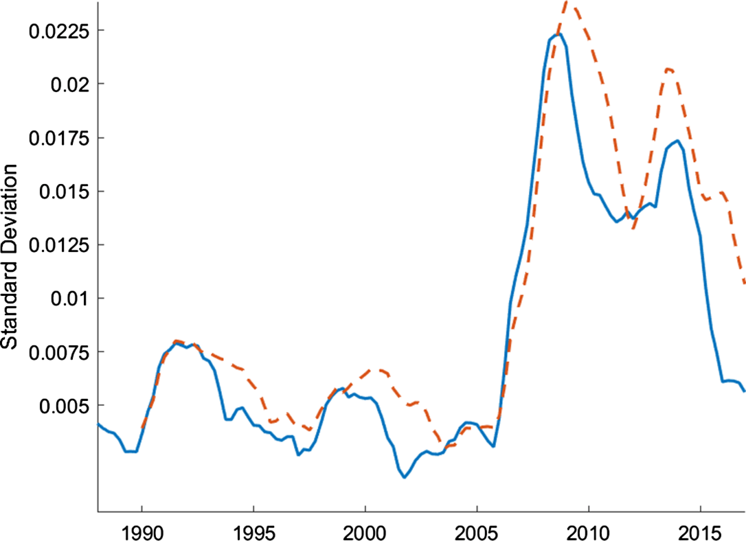
Figure 1. Rolling standard deviations of house price growth.
Note: The figure plots 4-yr (solid blue line) and 6-yr (dashed red line) rolling standard deviations of house price growth which is defined as the log differences in the quarterly averages of monthly Fannie Mac House Price. The data are seasonally adjusted and deflated by the GDP deflator.
To study time-varying volatility of house prices more rigorously, we estimate a reduced-form model with stochastic volatility.Footnote 9 Similar to our theoretical model, this approach allows the standard deviation of house prices to drift over time. The reduced form model is defined as
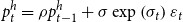 \begin{equation} p^h_t= \rho p^h_{t-1} + \sigma \exp \left (\sigma _t\right ) \varepsilon _t \end{equation}
 \begin{equation} \log \sigma _{t}=\rho _\sigma \log \sigma _{t-1}+(1-\rho _{\sigma }^{2})^{\frac{1}{2}}\eta u_{t} \end{equation}
where $p^h_t$
represents the growth rate of house prices,
$p^h_t$
represents the growth rate of house prices, $\sigma$
represents the steady state standard deviation of the innovation, and
$\sigma$
represents the steady state standard deviation of the innovation, and $\sigma _t$
represents the time-varying component of the standard deviation. As equations (1) and (2) show, both the growth rate,
$\sigma _t$
represents the time-varying component of the standard deviation. As equations (1) and (2) show, both the growth rate, $p^h_t$
, and the standard deviation of shock innovations,
$p^h_t$
, and the standard deviation of shock innovations, $\sigma _t$
, follow AR(1) processes.
$\sigma _t$
, follow AR(1) processes.
The reduced form model is estimated using flat priors and house price growth data for 1984:Q1–2017:Q1 that are the same as the data used to estimate the DSGE model.Footnote 10 As Table 1 shows, house prices exhibit persistent time-varying volatility. In particular, the standard deviation of the stochastic volatility shock follows an AR(1) process with a persistence, $\rho _\sigma$
, of 0.95 and a standard deviation,
$\rho _\sigma$
, of 0.95 and a standard deviation, $\eta$
, of 0.4 at the posterior mode.
$\eta$
, of 0.4 at the posterior mode.
In order to see the time-varying nature of house price volatility, it is helpful to analyze the underlying states for the stochastic volatility shock, which are calculated using a particle filter. As can be seen in Figure 2, the standard deviation shows two distinct increases, with one occurring in the early 1990s and the other occurring between 2005 and 2015. These changes in the standard deviation provide further evidence that there is in fact time-varying volatility in house prices.
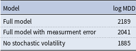
The inclusion of stochastic volatility in the reduced form model greatly improves the model fit. Table 2 shows that the log marginal data density (MDD) for the model with stochastic volatility is much larger than the model without stochastic volatility, supporting the inclusion of stochastic volatility in the analysis.
Table 1. Prior and posterior distribution: reduced form estimate
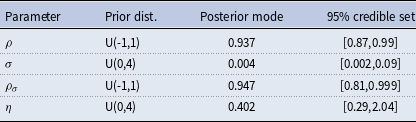
Note: U(a,b) represents the uniform distribution with lower bound a and upper bound b. The credible set is calculated around the median of the distribution.
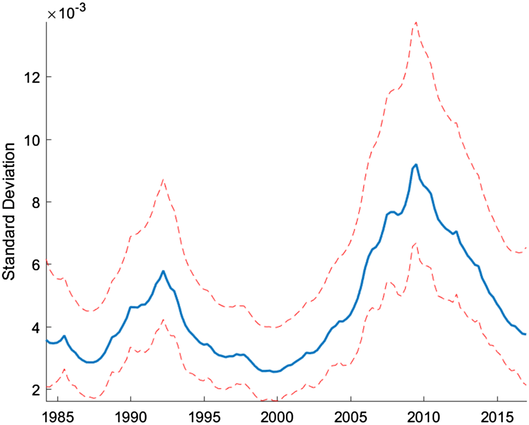
Figure 2. Underlying states: reduced form estimation.
Note: Smoothed underlying states are calculated at the posterior mode and are transformed to show the standard deviation of the innovation to the level shock. The median filtered states are shown along with the 5th and 95th percentiles.
While stochastic volatility has a direct link to uncertainty, they are not entirely identical. Here, we calculate a measure of uncertainty for house price growth following the methodology outlined by Jurado et al. (Reference Jurado, Ludvigson and Ng2015).Footnote 11 Based on this methodology, we calculate uncertainty as the 3-month ahead conditional volatility of the purely unforecastable component of house price growth which can be written as follows.Footnote 12
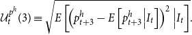 \begin{equation} \mathcal{U}^{p^h}_t (3) \equiv \sqrt{E \left [ \!\left (p^h_{t+3} - E \left [p^h_{t+3} \Big| I_t\right ] \right )^2 \Big|I_t\right ]}. \end{equation}
We need a large data set to help create an appropriate information set, $I_t,$
that allows us to strip away the forecasted future values of house price growth,
$I_t,$
that allows us to strip away the forecasted future values of house price growth, $E [p^h_{t+3} | I_t ]$
. Therefore, we use monthly data from January 1984 to December 2917 from McCracken and Ng (Reference McCracken and Ng2016) to supplement the house price growth data. As can be seen in Figure 3, there are significant swings in uncertainty about house price growth, with notable increases occurring around the start of 1990s and 2000s, and also during the house price boom and bust cycle of the Great Recession. While more volatile than the underlying states of the stochastic volatility estimate shown in Figure 2, the two series follow broadly similar paths.
$E [p^h_{t+3} | I_t ]$
. Therefore, we use monthly data from January 1984 to December 2917 from McCracken and Ng (Reference McCracken and Ng2016) to supplement the house price growth data. As can be seen in Figure 3, there are significant swings in uncertainty about house price growth, with notable increases occurring around the start of 1990s and 2000s, and also during the house price boom and bust cycle of the Great Recession. While more volatile than the underlying states of the stochastic volatility estimate shown in Figure 2, the two series follow broadly similar paths.
Table 2. Model fit: reduced form estimate
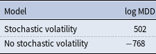

Figure 3. House price uncertainty.
Note: Uncertainty of house price growth measured using the methodology of Jurado et al. (Reference Jurado, Ludvigson and Ng2015) for the period of january 1984:Q1 to December 2017. The 3-month ahead uncertainty is presented.
Table 3. Prior and posterior distribution: reduced form estimates
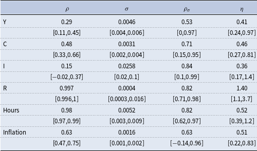
Note: 95% credible set centered around the median is quoted underneath the posterior mode.
Table 4. Model fit: reduced form estimate
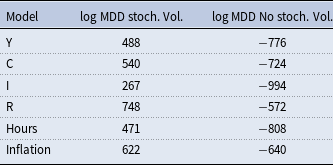
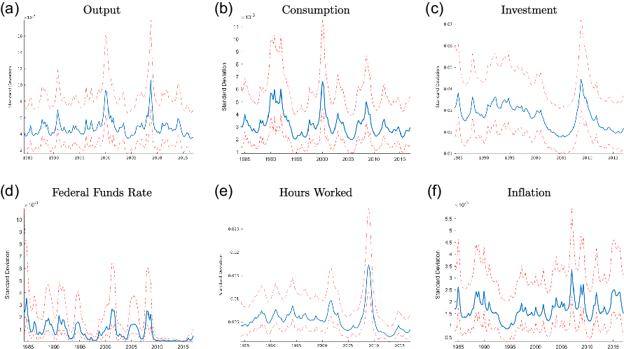
Figure 4. Underlying states: reduced form estimation.
Note: Smoothed underlying states are calculated at the posterior mode and are transformed to show the standard deviation of the innovation to the level shock. The median filtered states are shown along with the 5th and 95th percentiles.
The stochastic volatility in house prices is our main contribution, and therefore we highlight it more in this section. However, as shown in the literature (for instance, Justiniano and Primiceri (Reference Justiniano and Primiceri2008), Christiano et al. (Reference Christiano, Motto and Rostagno2014), Fernández-Villaverde et al. (Reference Fernández-Villaverde, Guerrón-Quintana, Kuester and Rubio-Ramírez2015a), Caldara et al. (Reference Caldara, Fuentes-Albero, Gilchrist and Zakrajšek2016), Bloom et al. (Reference Bloom, Floetotto, Jaimovich, Saporta-Eksten and Terry2018), and Davig and Foerster (Reference Davig and Foerster2018), among others), other macroeconomic variables also exhibit stochastic volatility. Table 3 reports the results for some of the most important macroeconomic series using the same approach as in equations (1) and (2). As can be seen in this table, output, consumption, investment, interest rates, labor hours, and inflation display time-varying volatility as well. Moreover, the inclusion of stochastic volatility improves the model fit for all these variables (Table 4).
The underlying states for output, consumption, investment, interest rates, labor hours, and inflation can be seen in Figure 4. While there is clear evidence of time-varying volatility, the pattern for each series looks different than the time-varying volatility for house prices. None of these series have a sustained increase in volatility in the 2000s that starts as early as house prices, which sees an increase in volatility starting at the start of the decade.
3. Model
The empirical section serves as a motivation where we show the existence of stochastic volatility in house prices, complementing other empirical studies. In addition to house price growth, many other economic indicators exhibit time-varying volatility, which are often correlated. These correlations can make identification very difficult in empirical models. Using a theoretical framework helps solve this problem. In particular, while the shocks are uncorrelated, such correlations in macroeconomic variables help to identify the parameters in our theoretical model. Moreover, our theoretical framework also helps disentangle the changes in financial frictions from elevated uncertainty which are highly correlated (Caldara et al. (Reference Caldara, Fuentes-Albero, Gilchrist and Zakrajšek2016)). To achieve all of these goals and to better understand the economic importance of time-varying volatility in house prices, we introduce stochastic volatility into a standard DSGE model with housing and collateralized borrowing as in Iacoviello (Reference Iacoviello2005), Liu et al. (Reference Liu, Wang and Zha2013), and Sapci (Reference Sapci2017). While many theoretical papers have focused on the effects of stochastic volatility, the literature has largely omitted the housing sector as a channel that can create and amplify the effects of such volatility (for instance, Justiniano and Primiceri (Reference Justiniano and Primiceri2008), Christiano et al. (Reference Christiano, Motto and Rostagno2014), Fernández-Villaverde et al. (Reference Fernández-Villaverde, Guerrón-Quintana, Kuester and Rubio-Ramírez2015a), Caldara et al. (Reference Caldara, Fuentes-Albero, Gilchrist and Zakrajšek2016), Bloom et al. (Reference Bloom, Floetotto, Jaimovich, Saporta-Eksten and Terry2018), and Davig and Foerster (Reference Davig and Foerster2018), among others).
The economy in the model is populated by five types of agents: unconstrained households, constrained households, entrepreneurs, retailers, and a central bank. Both households and entrepreneurs are infinitely lived with a measure of one, and there is a continuum of retailers of mass 1. Unconstrained households are assumed to own the retailers.Footnote 13
3.1 Entrepreneurs
Entrepreneurs produce a homogeneous intermediate good, $Y_{t}$
, with a wholesale price of
$Y_{t}$
, with a wholesale price of $P^{w}$
using the technology in equation (4) where K is the capital stock, h is the real estate input, and
$P^{w}$
using the technology in equation (4) where K is the capital stock, h is the real estate input, and $L_{u}$
and
$L_{u}$
and $L_{c}$
are unconstrained and constrained household labor supply, respectively. They sell their intermediate goods to retailers who transform them into final goods of price
$L_{c}$
are unconstrained and constrained household labor supply, respectively. They sell their intermediate goods to retailers who transform them into final goods of price $P_{t}$
.
$P_{t}$
.
 \begin{equation} Y_{t}=A_{t}K_{t-1}^{\mu }h_{t-1}^{\nu }L_{u,t}^{ \alpha (1-\mu -\nu )}L_{c,t}^{ (1-\alpha )(1-\mu -\nu )} \end{equation} $\mu \geq 0$
and
$\mu \geq 0$
and $\nu \geq 0$
denote the shares of capital and commercial real estates in production, respectively.
$\nu \geq 0$
denote the shares of capital and commercial real estates in production, respectively. $\alpha$
measures the relative size of unconstrained households to constrained households.
$\alpha$
measures the relative size of unconstrained households to constrained households. $A_{t}$
is the TFP that follows the process in equation (5).
$A_{t}$
is the TFP that follows the process in equation (5).
 \begin{equation} \log A_{t}=\bar{a}+\log A_{t-1}+\sigma _{a}\sigma _{a,t}\varepsilon _{a,t} \end{equation}
The standard deviation of the TFP follows:
 \begin{equation} \log \sigma _{A,t}=\upsilon _{A}\log \sigma _{A,t-1}+(1-\upsilon _{A}^{2})^{\frac{1}{2}}\eta _{A}u_{A,t}. \end{equation}
Entrepreneurs maximize their consumption, $c_t$
subject to equations (4)–(17) where
$c_t$
subject to equations (4)–(17) where $\zeta$
governs the degree of habit formation in consumption and
$\zeta$
governs the degree of habit formation in consumption and $\gamma$
is the discount rate.
$\gamma$
is the discount rate.
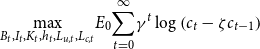 \begin{equation*} \underset {B_{t},I_{t},K_{t},h_{t},L_{u,t},L_{c,t}}{\max }E_{0}\overset {\infty }{\underset {t=0}{\sum }}\gamma ^{t}\log \left ( c_{t}-\zeta c_{t-1}\right ) \end{equation*}
 \begin{equation} \frac{Y_{t}}{X_{t}}+b_{t}=c_{t}+q_{t}\left ( h_{t}-h_{t-1}\right ) +\frac{R_{t-1}}{\pi _{t}}b_{t-1}+w_{t}^{u }L_{t}^{u }+w_{t}^{c }L_{t}^{c }+\frac{I_{t}}{\chi _{t}}+\xi _{h,t} +\xi _{k,t} \end{equation}
In the entrepreneur’s flow of funds above, $b_t$
denotes the entrepreneurial borrowing and
$b_t$
denotes the entrepreneurial borrowing and $R_{t-1}$
is the nominal interest rate on loans between t-1 and t. Consumption and investment goods are priced at
$R_{t-1}$
is the nominal interest rate on loans between t-1 and t. Consumption and investment goods are priced at $P_{t}$
and house price is
$P_{t}$
and house price is $Q_{t}$
. Therefore, the real house price is
$Q_{t}$
. Therefore, the real house price is $q_t=\frac{Q_t}{P_t},$
and the relative price is
$q_t=\frac{Q_t}{P_t},$
and the relative price is $\frac{1}{X_t}=\frac{P^{w}_t}{P_t}$
where
$\frac{1}{X_t}=\frac{P^{w}_t}{P_t}$
where $X_t$
is the markup of final goods over intermediate goods. The real wage is
$X_t$
is the markup of final goods over intermediate goods. The real wage is $w_{i,t}=\frac{W_{i,t}}{P_{i,t}}$
where
$w_{i,t}=\frac{W_{i,t}}{P_{i,t}}$
where $i=u,c$
and
$i=u,c$
and $\pi _{t}=\frac{P_{t}}{P_{t-1}}$
is the gross inflation rate. The adjustment costs of capital and housing are
$\pi _{t}=\frac{P_{t}}{P_{t-1}}$
is the gross inflation rate. The adjustment costs of capital and housing are
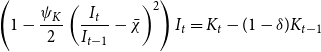
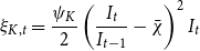 \begin{equation} \xi _{K,t}=\frac{\psi _{K}}{2}\left ( \frac{I_{t}}{I_{t-1}}-\bar{\chi }\right ) ^{2}I_{t} \end{equation}
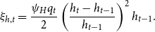 \begin{equation} \xi _{h,t}=\frac{\psi _{H}q_{t}}{2}\left ( \frac{h_{t}-h_{t-1}}{h_{t-1}}\right ) ^{2}h_{t-1}. \end{equation}
Similar to constrained borrowers, entrepreneurs can only borrow up to the expected future value of their total assets, which includes their physical capital as well as their commercial real estate. Following Liu et al. (Reference Liu, Wang and Zha2013), the borrowing constraint of the entrepreneurs is given by
 \begin{equation} R_{t}b_{t}\leq m_{t}E_t\!\left\{\left ( q_{t+1}h_{t}+u_{t+1}K_{t}\right )\pi _{t+1} \right\} \end{equation}
where $u_t$
is the shadow price of capital in consumption units. Given the assumption that
$u_t$
is the shadow price of capital in consumption units. Given the assumption that $\beta _u\gt \gamma$
, entrepreneurs’ borrowing constraint always binds.Footnote 14 There is a collateral constraint shock,
$\beta _u\gt \gamma$
, entrepreneurs’ borrowing constraint always binds.Footnote 14 There is a collateral constraint shock, $m_t,$
that allows for exogenous time variation in credit conditions. The shock is defined by the following process
$m_t,$
that allows for exogenous time variation in credit conditions. The shock is defined by the following process
 \begin{equation} \log m_t = \bar{m} +\log m_{t-1} + \sigma _m \sigma _{m,t}\varepsilon{m,t}. \end{equation}
As with other shocks in the model, the inclusion of stochastic volatility allows the standard deviation of the exogenous shock to drift over time. The process for the stochastic volatility of the shock is defined by
 \begin{equation} \log \sigma _{m,t}=\upsilon _{m}\log \sigma _{m,t-1}+(1-\upsilon _{m}^{2})^{\frac{1}{2}}\eta _{m}u_{m,t}. \end{equation}
The law of motion for capital is described in equation (13), where $ \chi$
is an investment-specific technology shock which is given in equation (14) with stochastic volatility shown in equation (15).
$ \chi$
is an investment-specific technology shock which is given in equation (14) with stochastic volatility shown in equation (15).
 \begin{equation} \left ( 1-\frac{\psi _{K}}{2}\left ( \frac{I_{t}}{I_{t-1}}-\bar{\chi }\right ) ^{2}\right ) I_{t}=K_{t}-(1-\delta )K_{t-1} \end{equation}
 \begin{equation} \log \chi _{t}=\bar{\chi }+\log \chi _{t-1}+\sigma _{\chi }\sigma _{\chi,t}\varepsilon _{\chi,t} \end{equation}
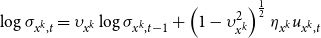 \begin{equation} \log{\sigma _{x^{k},t}}=\upsilon _{x^{k}}\log{\sigma _{x^{k},t-1}}+\left (1-\upsilon _{x^{k}}^{2}\right )^{\frac{1}{2}}\eta _{x^{k}}u_{x^{k},t} \end{equation}
The growth of the economy is defined as
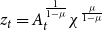 \begin{equation} z_{t}=A_{t}^{\frac{1}{1-\mu }}\chi ^{\frac{\mu }{1-\mu }} \end{equation}
where the growth rate is equal to
 \begin{equation} \bar{z}=\frac{\bar{a}+\mu \bar{\chi }}{1-\mu }. \end{equation}
3.2 Unconstrained households
There is a continuum of unconstrained households indexed by subscript $u$
, who maximize their consumption
$u$
, who maximize their consumption $c_{u,t}$
, housing services
$c_{u,t}$
, housing services $h_{u,t}$
, leisure
$h_{u,t}$
, leisure $1-l_{u,t}$
, and money holdings
$1-l_{u,t}$
, and money holdings $\frac{M_{u,t}}{P_{t}}$
subject to their budget constraint in equation (24).
$\frac{M_{u,t}}{P_{t}}$
subject to their budget constraint in equation (24).
 \begin{equation*} \underset {c_{u,t},b_{u,t},h_{u,t},L_{u,t},\frac {M_{u,t}}{P_{t}}}{\max }E_{0}\underset {t=0}{\overset {\infty }{\sum }}\varrho _{t}\beta _u ^{t}\left ( \log \left ( c_{u,t}-\zeta c_{u,t-1}\right ) +j_{u,t}\log h_{u,t}-\varphi _{t}\frac {\left ( L_{u,t}\right ) ^{\eta _u }}{\eta _u }+{\chi _u}\ln \frac {M_{u,t}}{P_{t}}\right ) \end{equation*}
Here $\beta _u$
denotes the discount factor of unconstrained households. The households face an intertemporal preference shock,
$\beta _u$
denotes the discount factor of unconstrained households. The households face an intertemporal preference shock, $\varrho _{t}$
, an intratemporal preference shock (intratemporal aggregate labor supply shock),
$\varrho _{t}$
, an intratemporal preference shock (intratemporal aggregate labor supply shock), $\varphi _{t}$
, and a housing demand shock,
$\varphi _{t}$
, and a housing demand shock, $ j_{u,t}$
, all of which follow the AR(1) processes as shown in equations (18), (19), and (20), respectively.
$ j_{u,t}$
, all of which follow the AR(1) processes as shown in equations (18), (19), and (20), respectively.
 \begin{equation} \log \varrho _{t}=\rho _{\varrho }\log \varrho _{t-1}+\sigma _{\varrho }\sigma _{\varrho,t}\varepsilon _{\varrho,t} \end{equation}
and
 \begin{equation} \log{j}_{t}=\rho _{j}\log{j}_{t-1}+\sigma _{j}\sigma _{j,t}\varepsilon _{j,t} \end{equation}
and
 \begin{equation} \log \varphi _{t}=\rho _{\varphi }\log \varphi _{t-1}+\sigma _{\varphi }\sigma _{\varphi,t}\varepsilon _{\varphi,t} \end{equation}
The standard deviation of the innovations follow:
 \begin{equation} \log \sigma _{\varrho,t}=\upsilon _{\varrho }\log \sigma _{\varrho,t-1}+(1-\upsilon _{\varrho }^{2})^{\frac{1}{2}}\eta _{\varrho }u_{\varrho,t} \end{equation}
and
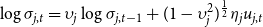 \begin{equation} \log \sigma _{j,t}=\upsilon _{j}\log \sigma _{j,t-1}+(1-\upsilon _{j}^{2})^{\frac{1}{2}}\eta _{j}u_{j,t} \end{equation}
and
 \begin{equation} \log \sigma _{\varphi,t}=\upsilon _{\varrho }\log \sigma _{\varphi,t-1}+(1-\upsilon _{\varphi }^{2})^{\frac{1}{2}}\eta _{\varphi }u_{\varphi,t}. \end{equation}
The budget constraint is
 \begin{equation} c_{u,t}+q_{t}\left ( h_{u,t}-h_{u,t-1}\right ) +\frac{R_{t-1}}{\pi _{t}}b_{u,t-1}+\xi _{e,t}=b_{u,t}+w_{u,t}L_{u,t}+F_{t}+T_{u,t}-\frac{M_{u,t}-M_{u,t-1}}{P_{t}}. \end{equation}
where $F_{t}$
is the dividends received from retailers,
$F_{t}$
is the dividends received from retailers, $\xi _{e,t}$
is the sum of adjustment costs, and
$\xi _{e,t}$
is the sum of adjustment costs, and $\frac{M_{u,t}}{P_{t}}$
is the real money balances.
$\frac{M_{u,t}}{P_{t}}$
is the real money balances. $T_{u,t}-\frac{M_{u,t}-M_{u,t-1}}{P_{t}}$
denotes the net transfers from the central bank financed by printing money. Since the paper focuses on monetary rules that target interest rates, the quantity of money has no implications for the rest of the model, given that the utility is separable in money balances.
$T_{u,t}-\frac{M_{u,t}-M_{u,t-1}}{P_{t}}$
denotes the net transfers from the central bank financed by printing money. Since the paper focuses on monetary rules that target interest rates, the quantity of money has no implications for the rest of the model, given that the utility is separable in money balances.
3.3 Constrained households
Similar to unconstrained households, constrained households also choose their optimal consumption, $c_{c,t}$
, and leisure,
$c_{c,t}$
, and leisure, $1-L_{c,t}$
, subject to their budget constraint given in equation (25). They invest in the housing market, where they receive utility from housing services. Differently from unconstrained households, they are subject to the borrowing constraint in equation (26) and do not value the future as much. In particular,
$1-L_{c,t}$
, subject to their budget constraint given in equation (25). They invest in the housing market, where they receive utility from housing services. Differently from unconstrained households, they are subject to the borrowing constraint in equation (26) and do not value the future as much. In particular, $\beta _{u}\gt \beta _{c}$
.Footnote 15
$\beta _{u}\gt \beta _{c}$
.Footnote 15
 \begin{equation*} \underset{c_{c,t},b_{c,t},h_{c,t},L_{c,t},\frac{M_{c,t}}{P_{t}}}{\max }E_{0}\underset{t=0}{\overset{\infty }{\sum }\varrho _{t}}\beta_c^{t}\left( \log\!\left( c_{c,t}-\zeta c_{c,t-1}\right) +j_{c,t}\log h_{c,t}-\varphi _{t}\frac{\left(L_{c,t}\right) ^{\eta_c}}{\eta_c}+\chi_c\ln \frac{M_{c,t}}{P_{t}}\right) \end{equation*}
The constrained households also face an intertemporal preference shock, $\varrho _{t}$
, an intratemporal preference shock (intratemporal aggregate labor supply shock),
$\varrho _{t}$
, an intratemporal preference shock (intratemporal aggregate labor supply shock), $\varphi _{t}$
, and a housing shock
$\varphi _{t}$
, and a housing shock $j_{c,t}$
which follow the same processes as in the case for the unconstrained households. Constrained households pay for their consumption, housing investment, and debt payment from previous period using their labor income and borrowings from the current period, as shown in equation (25).
$j_{c,t}$
which follow the same processes as in the case for the unconstrained households. Constrained households pay for their consumption, housing investment, and debt payment from previous period using their labor income and borrowings from the current period, as shown in equation (25).
 \begin{equation} c_{c,t}+q_{t}\left ( h_{c,t}-h_{c,t-1}\right ) +\frac{R_{t-1}}{\pi _{t}}b_{c,t-1}+\xi _{e,t}=b_{c,t}+w_{c,t}L_{c,t}- \frac{M_{c,t}-M_{c,t-1}}{P_{t}} +T_{c,t} \end{equation}
The constrained households need some of their assets to be collateralized to purchase housing, which restrains the amount of available credit to the borrowers. The borrowing constraint in equation (26) shows that the repayment of the household’s debt cannot exceed the expected future value of the real estate bought at time $t$
.
$t$
.
 \begin{equation} R_{t}b_{c,t}\leq m_{c,t}E_{t}\!\left \{ q_{t+1}h_{c,t}\pi _{t+1}\right \} \end{equation}
3.4 Retailers
Following Bernanke et al. (Reference Bernanke, Gertler, Gilchrist, Bernanke, Gertler and Gilchrist1999) and Iacoviello (Reference Iacoviello2005), retailers transform the intermediate goods into a composite final good, $Y_{t}$
, where
$Y_{t}$
, where $ Y_{t}^{f}=\left ( \underset{0}{\overset{1}{\int }}Y_{t}(z)^\frac{\varepsilon -1}{\varepsilon }dz\right ) ^{\frac{\varepsilon }{\varepsilon -1 }}$
and sell it at the price
$ Y_{t}^{f}=\left ( \underset{0}{\overset{1}{\int }}Y_{t}(z)^\frac{\varepsilon -1}{\varepsilon }dz\right ) ^{\frac{\varepsilon }{\varepsilon -1 }}$
and sell it at the price $P_{t}(z)$
where
$P_{t}(z)$
where $P_{t}=\left ( \underset{0}{\overset{1}{\int }}P_{t}(z)^{1-\varepsilon }dz\right ) ^{\frac{1}{1-\varepsilon }}$
.
$P_{t}=\left ( \underset{0}{\overset{1}{\int }}P_{t}(z)^{1-\varepsilon }dz\right ) ^{\frac{1}{1-\varepsilon }}$
.
Each retailer faces the following individual demand curve:
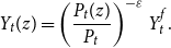 \begin{equation*} Y_{t}(z)=\left ( \frac {P_{t}(z)}{P_{t}}\right ) ^{-\varepsilon }Y_{t}^{f}. \end{equation*}
The sale price, $P_{t}(z)$
, can be changed in every period with a probability of
$P_{t}(z)$
, can be changed in every period with a probability of $1-\theta .$
The optimal price
$1-\theta .$
The optimal price $P_{t}^{\ast }(z)$
solves
$P_{t}^{\ast }(z)$
solves
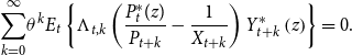 \begin{equation*} \underset {k=0}{\overset {\infty }{\sum }}\theta ^{k}E_{t}\left \{ \Lambda _{t,k}\left ( \frac {P_{t}^{\ast }(z)}{P_{t+k}}-\frac {1}{X_{t+k}}\right ) Y_{t+k}^{\ast }\left ( z\right ) \right \} =0. \end{equation*}
where $\Lambda _{t,k}=\beta _u ^{^k}\frac{\lambda _{u,t+k}}{\lambda _{u,t}}$
is the patient households’ relevant discount factor and
$\Lambda _{t,k}=\beta _u ^{^k}\frac{\lambda _{u,t+k}}{\lambda _{u,t}}$
is the patient households’ relevant discount factor and $X_{t}$
is the markup. The evolution of prices are as follows:
$X_{t}$
is the markup. The evolution of prices are as follows:
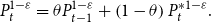 \begin{equation} P_{t}^{1-\varepsilon }=\theta P_{t-1}^{1-\varepsilon }+\left ( 1-\theta \right ) P_{t}^{*1-\varepsilon }. \end{equation}
3.5 Central bank
The central bank adjusts the nominal interest rate using the following Taylor rule.
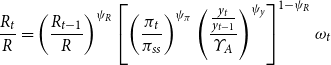 \begin{equation} \frac{R_{t}}{R}=\left (\frac{R_{t-1}}{R}\right )^{\psi _{R}}\left [\left (\frac{\pi _{t}}{\pi _{ss}}\right )^{\psi _{\pi }}\left (\frac{\frac{y_{t}}{y_{t-1}}}{\varUpsilon _{A}}\right )^{\psi _{y}}\right ]^{1-\psi _{R}}\omega _{t} \end{equation}
where $\omega _{t}$
represents the monetary policy shock which can be shown as
$\omega _{t}$
represents the monetary policy shock which can be shown as
 \begin{equation} \log{\omega _{t}}=\sigma _{\omega }\sigma _{\omega,t}\varepsilon _{\omega,t} \end{equation}
where $\sigma _{\omega,t}$
follows
$\sigma _{\omega,t}$
follows
 \begin{equation} \log{\sigma _{\omega,t}}=\varrho _{\omega }\log{\sigma _{\omega,t-1}}+\left (1-\upsilon _{\omega }^{2}\right )^{\frac{1}{2}}\eta _{\omega }u_{\omega,t}. \end{equation}
3.6 Market equilibrium
The resource constraint is shown in equation (31).
 \begin{equation} Y_{t}=c_{t}+c_{u,t}+c_{c,t}+\frac{I_{t}}{\chi _{t}}+\xi _{e,t} \end{equation}
Additionally, labor and loans markets clear when supply is equal to demand in respective markets.
 \begin{equation} b_{t}+b_{u,t}+b_{c,t}=0 \end{equation}
Finally, land supply is fixed as shown in equation (33).Footnote 16
 \begin{equation} h_{t}+h_{u,t}+h_{c,t}=1 \end{equation}
4. Data and priors
The data used to estimate the model span from 1984:Q1 to 2017:Q1.Footnote 17 In particular, we use seven data series: growth rate of real output, growth rate of real per capita investment, growth rate of real per capita consumption, the log of hours worked, inflation (measured as the logged ratio of the price level of the current and previous period), the log of the gross federal funds rate, and the growth rate of house prices.Footnote 18
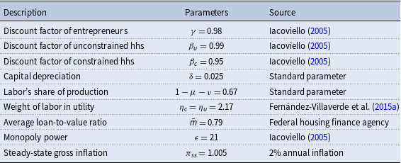
The parameters of the model are divided into estimated and fixed parameters. The priors of the estimated parameters are described in Table 5. These priors are similar to those that are used by Christiano et al. (Reference Christiano, Motto and Rostagno2014) and Del Negro et al. (Reference Del Negro, Giannone, Giannoni and Tambalotti2017). As discussed in Fernández-Villaverde et al. (Reference Fernández-Villaverde, Guerrón-Quintana, Kuester and Rubio-Ramírez2015a), it is difficult to determine appropriate priors for the stochastic volatility parameters, therefore, we use uninformative priors for them. To avoid potential identification issues and ease the computational burden, we fix some parameters to certain values which are described in Table 6. Among these parameters, capital depreciation, labor share of production, average loan to value (LTV) ratio, and steady-state gross inflation rate are based on US data and are commonly used in the literature as standard parameters. For instance, capital depreciation of 0.025 yields an annual depreciation of 10% as is commonly used in the literature. Labor share of production 67% matches the long-term US data obtained from the U.S. Bureau of Labor Statistics. Average LTV ratios of 79% is obtained from Federal Housing Agency’s Fannie Mae and Freddie Mac Public Dataset. The average LTV ratio is calibrated to many different values in the literature; however, the value we use is between 0.75 used by Liu et al. (Reference Liu, Wang and Zha2013) and 0.9 used by Guerrieri and Iacoviello (Reference Guerrieri and Iacoviello2017b). However, we change the value of the LTV ratio in Section 6.6.1 “The Role of the Credit Channel” to demonstrate the effects of this parameter on the economy. Lastly, steady state gross inflation of 1.005 yields a 2% annual inflation rate which has been a long-term target of the FED.Footnote 19
Table 5. Prior distributions
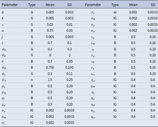
Table 6. Calibration
5. Estimation
While DSGE models have historically been solved using linear approximations, the nonlinear features of the model require a nonlinear approximation. A second-order approximation allows for clean identification of the parameters governing stochastic volatility and the shocks to stochastic volatility, without the need for measurement error as shown by Fernández-Villaverde et al. (Reference Fernández-Villaverde, Guerrón-Quintana, Kuester and Rubio-Ramírez2015a). While a third-order approximation has advantages over a second-order approximation, third-order approximation would require the addition of measurement errors. Measurement errors can have detrimental effects when estimating DSGE models (Canova et al. (Reference Canova, Ferroni and Matthes2014)) and can make identification of the stochastic volatility shocks difficult or impossible.Footnote 20 Additionally, using a third-order approximation or global approximation is not computationally feasible for a model this size.Footnote 21 The approximation of the model is then estimated using a particle filter and Metropolis–Hastings algorithm.
The estimation follows Fernández-Villaverde et al. (Reference Fernández-Villaverde, Guerrón-Quintana, Kuester and Rubio-Ramírez2015a), who show that many dynamic equilibrium models can be written as
 \begin{equation} \mathbb{E}_t f \left ( \mathcal{Y}_{t+1}, \mathcal{Y}_t,\mathcal{S}_{t+1}, \mathcal{S}_{t},\mathcal{Z}_{t+1}, \mathcal{Z}_t;\;\gamma \right )=0 \end{equation}
where $\mathbb{E}_t$
represents the conditional expectation operator at time t,
$\mathbb{E}_t$
represents the conditional expectation operator at time t, $\mathcal{Y}_t$
represents the
$\mathcal{Y}_t$
represents the $k$
x
$k$
x $1$
vector of observables at time
$1$
vector of observables at time $t,$
$t,$ $\mathcal{S}_{t}$
represents the
$\mathcal{S}_{t}$
represents the $n$
x
$n$
x $1$
vector of endogenous states at time time
$1$
vector of endogenous states at time time $t,$
$t,$ $\mathcal{Z}_{t}$
represents the
$\mathcal{Z}_{t}$
represents the $m$
x
$m$
x $1$
vector of structural shocks at time
$1$
vector of structural shocks at time $t$
,
$t$
, $\gamma$
represents the vector of parameters in the model, and f maps
$\gamma$
represents the vector of parameters in the model, and f maps $\mathbb{R}^{2(k+n+m)}$
into
$\mathbb{R}^{2(k+n+m)}$
into $\mathbb{R}^{k+n+m}.$
In this model, the endogenous state is defined as
$\mathbb{R}^{k+n+m}.$
In this model, the endogenous state is defined as
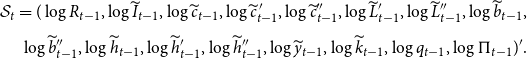 \begin{align} \mathcal{S}_{t}= (\log R_{t-1}, \log \widetilde{I}_{t-1},\log \widetilde{c}_{t-1},\log \widetilde{c}^{\,\prime}_{t-1},\log \widetilde{c}^{\prime\prime}_{t-1},\log \widetilde{L}^{\prime}_{t-1},\log \widetilde{L}^{\prime\prime}_{t-1},\log \widetilde{b}_{t-1}, \\[5pt] \nonumber \log \widetilde{b}^{\prime\prime}_{t-1},\log \widetilde{h}_{t-1},\log \widetilde{h}^{\prime}_{t-1},\log \widetilde{h}^{\prime\prime}_{t-1},\log \widetilde{y}_{t-1},\log \widetilde{k}_{t-1},\log q_{t-1},\log \Pi _{t-1})'. \end{align}
The observables are defined as
 \begin{equation*} \mathcal {Y}_t = \left ( \Delta \log \widetilde {y}_t, \Delta \log \widetilde {I}_t, \Delta \log \widetilde {c}_t, \Delta \log \widetilde {w}_t, \Delta \log \widetilde {q}_t, \Pi _t, R_t, \right )^{\prime}. \end{equation*}
The structural shocks are defined as
 \begin{equation*}\mathcal {Z}_{t} = ( \log \widetilde {\chi }_t, \log j_t, \log m_t, \log \widetilde {A}_t, \log {\omega,t}, \log \varrho _{t}, \log \varphi _{t})^{\prime}. \end{equation*}
The structural shocks are assumed to follow the process below.
 \begin{equation} \mathcal{Z}_{it+1}=\rho _i \mathcal{Z}_{it}+ \Lambda \sigma _i \sigma _{it+1}\epsilon _{it+1} \end{equation}
for all $i \in{1,\ldots,m}$
where
$i \in{1,\ldots,m}$
where $\sigma _{it+1}$
denotes the stochastic volatility shock and
$\sigma _{it+1}$
denotes the stochastic volatility shock and $\Lambda$
represents the perturbation parameter.Footnote 22 The stochastic volatility shocks evolve as
$\Lambda$
represents the perturbation parameter.Footnote 22 The stochastic volatility shocks evolve as
 \begin{equation} \log \sigma _{it+1}=\rho _{\sigma _i} \log \sigma _{it}+ \Lambda \left ( 1- \rho _{\sigma _i}^2 \right )^{\frac{1}{2}}\eta _i u_{it+1}. \end{equation}
Since there are an equal number of stochastic volatility shocks and observables, the particle filter described in Fernández-Villaverde et al. (Reference Fernández-Villaverde, Guerrón-Quintana, Kuester and Rubio-Ramírez2015a) can be applied directly to calculate the likelihood. In our analysis, we used 15,000 particles. As described in Herbst and Schorfheide (Reference Herbst and Schorfheide2015), the particle filter is modified to include a mutation resample-move step. The likelihood is combined with the prior in order to calculate the posterior needed for the Metropolis–Hastings algorithm which is run for 170,000 draws with the first 30,000 dropped as a burn-in sample.Footnote 23 Every 40th draw is kept; the remaining 3500 draws are used to calculate the posterior distribution and the model fit.Footnote 24
6. Results
6.1 Posterior distribution
Table 7 presents the posterior mode and standard deviations for each parameter.Footnote 25 One interesting result is the adjustment cost parameter for capital, $\psi _k$
, which is 4.403 at the posterior mode. Larger values associate with higher cost of adjusting investment, which might cause firms to reduce investment when they are less certain about future. Most of our estimates are at or near standard values, but the response of policy to output and inflation,
$\psi _k$
, which is 4.403 at the posterior mode. Larger values associate with higher cost of adjusting investment, which might cause firms to reduce investment when they are less certain about future. Most of our estimates are at or near standard values, but the response of policy to output and inflation, $\psi _y$
and
$\psi _y$
and $\psi _\pi$
, are higher than typical, but are similar to the values found by Plante et al. (Reference Plante, Richter and Throckmorton2017).
$\psi _\pi$
, are higher than typical, but are similar to the values found by Plante et al. (Reference Plante, Richter and Throckmorton2017).
Table 7. Posterior distribution
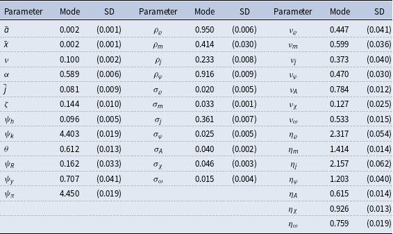
The third set of columns in Table 7 show the posteriors for the persistence, $\nu,$
and standard deviations,
$\nu,$
and standard deviations, $\eta,$
of the stochastic volatility processes.Footnote 26 All the values of the posterior modes are far from zero and are tightly identified, which suggests that stochastic volatility plays an important role in fitting the data.Footnote 27 The standard deviations of the stochastic volatility shocks for the intertemporal preference shock
$\eta,$
of the stochastic volatility processes.Footnote 26 All the values of the posterior modes are far from zero and are tightly identified, which suggests that stochastic volatility plays an important role in fitting the data.Footnote 27 The standard deviations of the stochastic volatility shocks for the intertemporal preference shock $\eta _\varrho$
, the housing demand shock
$\eta _\varrho$
, the housing demand shock $\eta _j$
, and the collateral shock
$\eta _j$
, and the collateral shock $\eta _m$
are the three largest of the stochastic volatility shocks. This finding is not surprising, because these shocks affect the demand for housing more directly than the rest (housing demand being the most direct driver) which can be helpful in explaining the observed time-varying volatility of house prices.
$\eta _m$
are the three largest of the stochastic volatility shocks. This finding is not surprising, because these shocks affect the demand for housing more directly than the rest (housing demand being the most direct driver) which can be helpful in explaining the observed time-varying volatility of house prices.
6.2 Model fit
We calculate the log marginal data densities (log MDD) of the model with and without stochastic volatility to compare the model fit.Footnote 28 Model comparison is difficult when comparing models with and without stochastic volatility.Footnote 29 One concern is that the alternative models need to assume there are measurement errors for all observables, while the model with stochastic volatility has no measurement error. To assuage concerns about measurement error, we calculate the model fit for the full model with and without measurement error. As in Gust et al. (Reference Gust, Herbst, López-Salido and Smith2017), the measurement error is assumed to be i.i.d. with a mean of zero and a normal distribution with a standard deviation set to 20% of the standard deviation of the actual data. As can be seen in Table 8, the baseline model with stochastic volatility fits the data far better than the model without stochastic volatility. The difference between the values gives a log Bayes factor of 304 when comparing the model without measurement error and 156 when comparing the model with measurement error.Footnote 30 This finding provides decisive evidence that including stochastic volatility allows the model to fit the data substantially better.
Table 8. Model fit
6.3 Underlying states
To better understand how the shocks of the model evolve over time, we measure the filtered states of the model.Footnote 31 Figure 5 shows the filtered underlying states of the traditional shocks in log deviation from the mean form. All the shocks, except technology shocks, show dramatic fluctuations during the Great Recession. In particular, the collateral constraint shock, $m$
, increases pre-recession, indicating the lax credit conditions during the housing boom and starts to decrease in early 2007 as credit conditions tightened during the financial crisis. The housing demand shock,
$m$
, increases pre-recession, indicating the lax credit conditions during the housing boom and starts to decrease in early 2007 as credit conditions tightened during the financial crisis. The housing demand shock, $j,$
steadily increases until the third quarter of 2006 when it begins to fall, reaching a trough in the first quarter of 2008, representing the bust in the housing market. Another shock with dramatic fluctuations is the intertemporal preference shock,
$j,$
steadily increases until the third quarter of 2006 when it begins to fall, reaching a trough in the first quarter of 2008, representing the bust in the housing market. Another shock with dramatic fluctuations is the intertemporal preference shock, $\varrho,$
which fell during the first part of the 2000s before hitting a trough in the fourth quarter of 2006 and increasing significantly in the following quarters. This is important for explaining the increase in lending and housing demand during the early 2000s when the intertemporal preference shock was low. The increase in the intertemporal preference shock in later periods, however, causes a decline in lending and house prices. We can also observe loose monetary policy during the early 2000s as the housing bubble formed, since the monetary policy shock,
$\varrho,$
which fell during the first part of the 2000s before hitting a trough in the fourth quarter of 2006 and increasing significantly in the following quarters. This is important for explaining the increase in lending and housing demand during the early 2000s when the intertemporal preference shock was low. The increase in the intertemporal preference shock in later periods, however, causes a decline in lending and house prices. We can also observe loose monetary policy during the early 2000s as the housing bubble formed, since the monetary policy shock, $\omega$
, was negative for multiple quarters in a row.
$\omega$
, was negative for multiple quarters in a row.
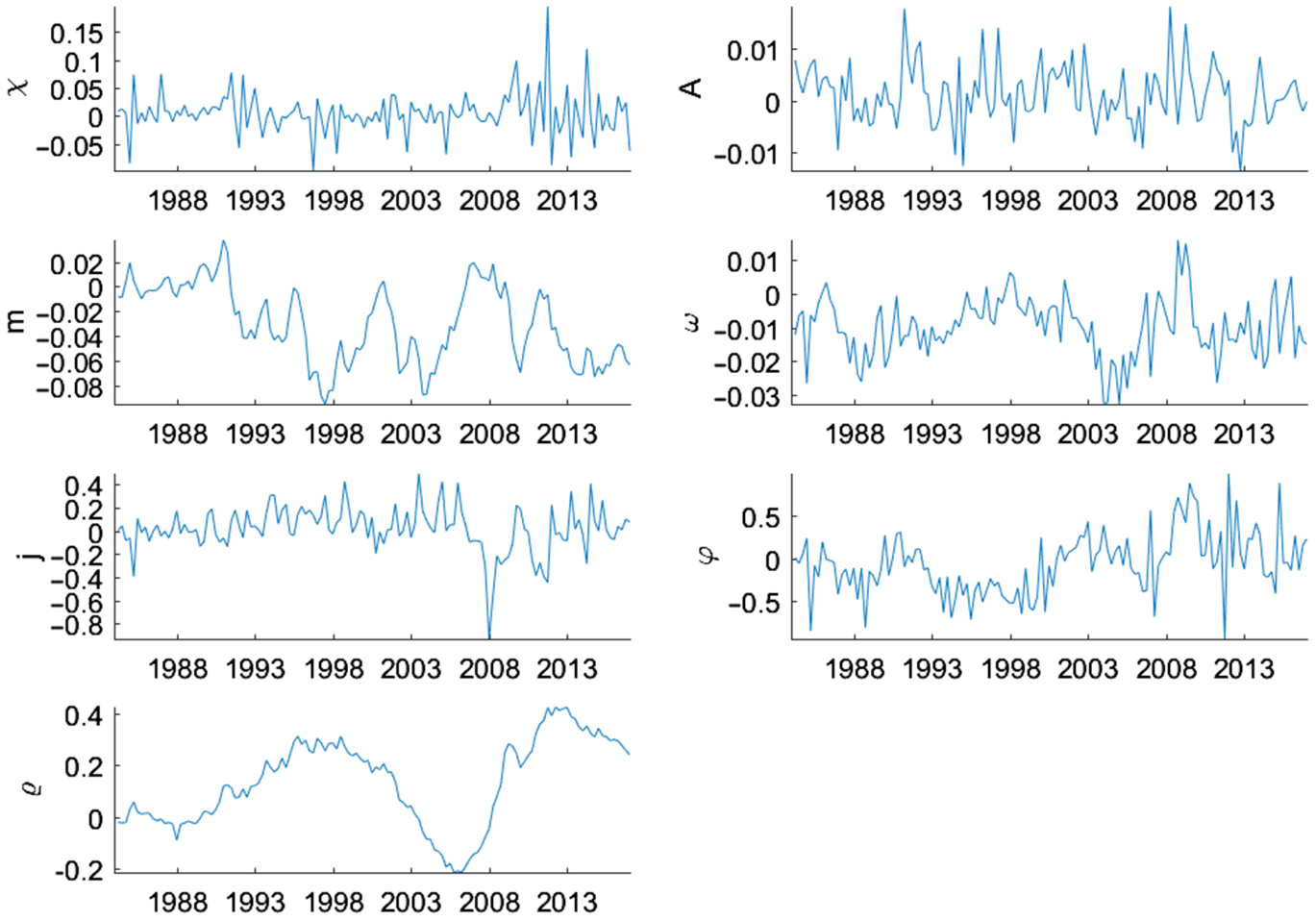
Figure 5. Underlying states: level shocks.
Note: Smoothed underlying states of the level shocks in log deviation from the mean form. They are calculated at the posterior mode. The median filtered states are shown.
Similarly, Figure 6 presents the smoothed underlying states of the stochastic volatility shocks in log deviation from the mean. Of particular interest are the large increases in the volatility of the housing demand, $j,$
and intertemporal preference,
$j,$
and intertemporal preference, $\varrho,$
shocks. The volatility of housing demand peaks in the fourth quarter of 2007, while intertemporal preference shock volatility has twin peaks in the first and fourth quarter of 2008, at the height of the financial crisis. Both shocks affect house prices more directly, therefore elevated volatility of these shocks would increase house price volatility. Interestingly, the volatility of the collateral constraint shock,
$\varrho,$
shocks. The volatility of housing demand peaks in the fourth quarter of 2007, while intertemporal preference shock volatility has twin peaks in the first and fourth quarter of 2008, at the height of the financial crisis. Both shocks affect house prices more directly, therefore elevated volatility of these shocks would increase house price volatility. Interestingly, the volatility of the collateral constraint shock, $m,$
increases slightly starting in 2007 before falling dramatically in 2009, which suggests that financial sector risk management measures were effective during that time period. The other shocks do not show much evidence of increased volatility during the Great Recession time period, with the volatility of the monetary policy shock,
$m,$
increases slightly starting in 2007 before falling dramatically in 2009, which suggests that financial sector risk management measures were effective during that time period. The other shocks do not show much evidence of increased volatility during the Great Recession time period, with the volatility of the monetary policy shock, $\omega,$
actually falling in 2007.
$\omega,$
actually falling in 2007.
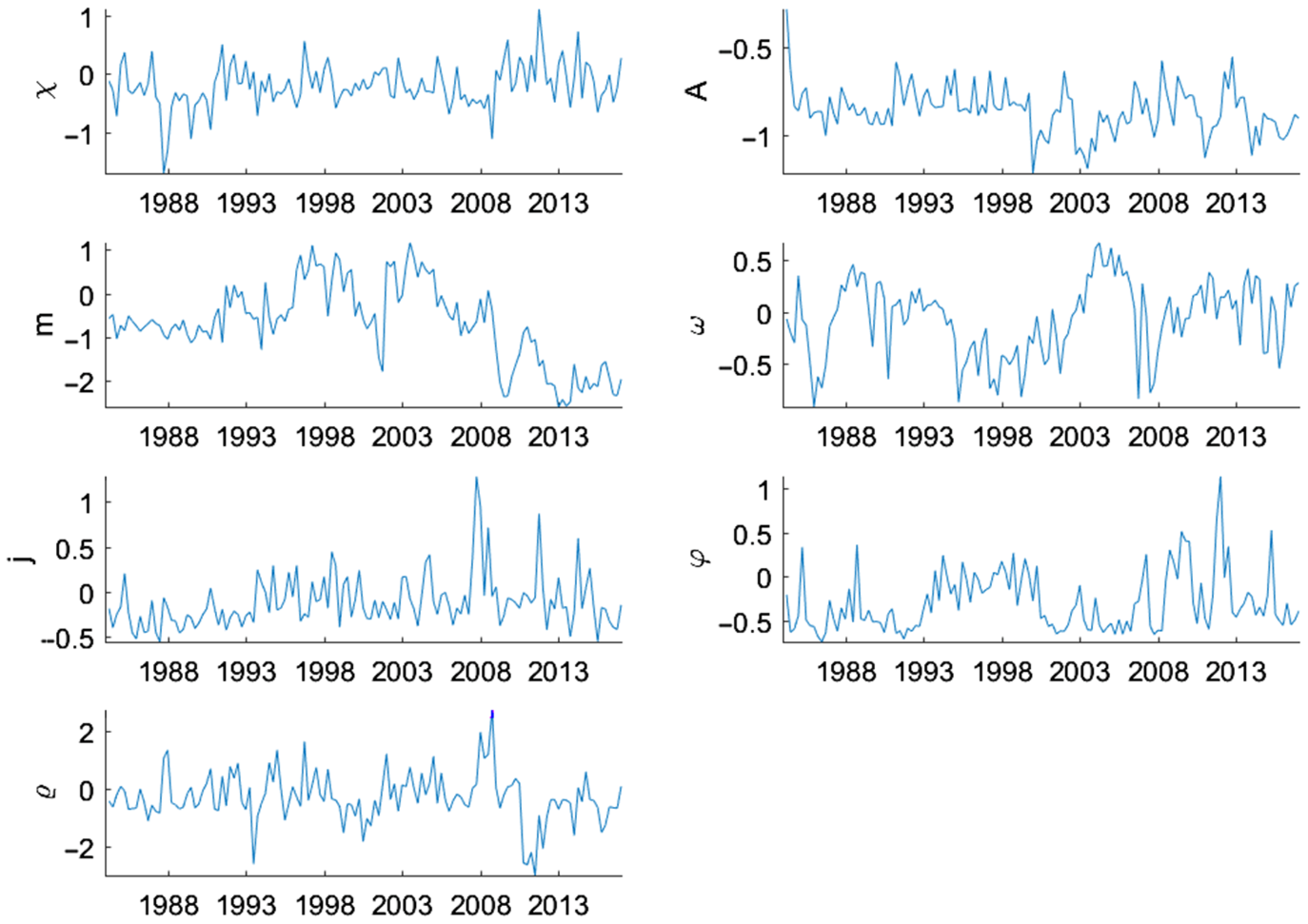
Figure 6. Underlying states: stochastic volatility.
Note: Smoothed underlying states of the stochastic volatility shocks in log deviation from the mean form. They are calculated at the posterior mode. The median filtered states are shown.
6.4 House price volatility
As the empirical analysis in Section 2 shows, there is a large increase in the volatility of house prices that began in 2008. We conduct a counterfactual study to better understand whether stochastic volatility shocks can explain the observed increase in house price volatility during the Great Recession. Therefore, the model is simulated with all the underlying states except the stochastic volatility shocks, which are all set to zero from the start of 2007 to the end of 2010. If the stochastic volatility shocks are not important for explaining the increase in house price volatility during this time, we should observe a negligible difference between the data and the counterfactual study.
Figure 7 shows how volatile house prices would have been during the Great Recession period if there were no stochastic volatility shocks from 2007 to 2010. As the comparison of the data and counterfactual study indicate, without stochastic volatility, house prices would have been much less volatile during this time. This analysis shows that stochastic volatility shocks played an important role in explaining the house price volatility during the Great Recession.
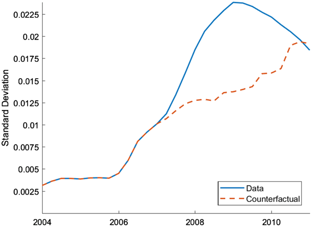
Figure 7. Counterfactual study: stochastic volatility.
Note: Rolling 6-year standard deviation of house price growth. The blue, solid line represents the actual data. The red, dashed line is generated from the simulated model using the underlying filtered shocks, except the stochastic volatility shocks, which are set to zero from 2007Q1 to 2010Q4.
6.5 Impulse responses
As shown in the above results, stochastic volatility is particularly important in fitting the model to data and largely contributes to the increase in house price volatility observed during the Great Recession. A natural question follows: how do these stochastic volatility shocks affect the economy? To answer this question, we obtain the generalized impulse response functions (GIRFs) using a third-order approximation as detailed in Andreasen et al. (Reference Andreasen, Fernández-Villaverde and Rubio-Ramírez2017) and calculate them using the posterior mode described in Section 6.1.
In this section, we first present the responses to level shocks to shed some light on the role the housing market plays as a propagation mechanism. We then answer the question about the impact of stochastic volatility on the economy.
6.5.1 Level shocks
To better understand the features of the model and the role of housing as a propagation mechanism, it is helpful to first look at the GIRFs for the level shocks in the model. Figure 8 presents the GIRFs of output, investment, house prices, and total loans to a one standard deviation increase in the innovations of the housing demand ( $j$
), collateral constraint (
$j$
), collateral constraint ( $m$
), intertemporal preference (
$m$
), intertemporal preference ( $\varrho$
), and monetary policy (
$\varrho$
), and monetary policy ( $\omega$
) shocks. The GIRFs for all other shocks can be seen in Figure A1 in Appendix A.5.
$\omega$
) shocks. The GIRFs for all other shocks can be seen in Figure A1 in Appendix A.5.
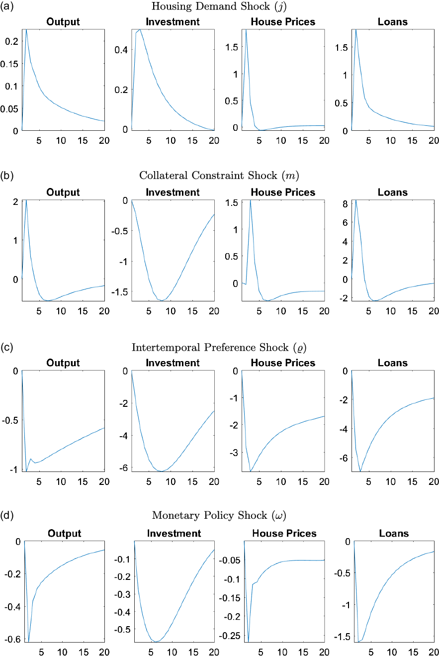
Figure 8. Responses of macroeconomic variables to select level shocks.
Note: The figure plots the generalized impulse responses of selected variables to a one standard deviation increase in innovation of correspondent shocks. The responses are calculated at the unconditional mean of the states. All responses are normalized so that the units of the vertical axis are percentage deviations from the steady-state.
A positive housing demand shock ( $j$
) causes households to receive higher utility from housing services, which in turn increases their demand and prices. Given that housing is used as collateral, higher prices increase the collateral value, creating more lax credit conditions for everyone. Better credit conditions allow borrowers to obtain more loans which helps increase their demand for housing, positively affecting prices further. The lax credit conditions also help entrepreneurs, who can now borrow more, and therefore, afford more capital goods. Overall, the positive effects coming from high house prices spill over to the real economy, increasing investment and output.
$j$
) causes households to receive higher utility from housing services, which in turn increases their demand and prices. Given that housing is used as collateral, higher prices increase the collateral value, creating more lax credit conditions for everyone. Better credit conditions allow borrowers to obtain more loans which helps increase their demand for housing, positively affecting prices further. The lax credit conditions also help entrepreneurs, who can now borrow more, and therefore, afford more capital goods. Overall, the positive effects coming from high house prices spill over to the real economy, increasing investment and output.
With a positive collateral constraint shock ( $m$
), borrowers can obtain loans using a larger portion of their house value (or lower down payment). Better credit conditions increase the demand for houses, and therefore, their prices. The higher demand for borrowing, however, increases the real interest rates which affects capital investment negatively. Given that housing is also used in production, the positive effects outweigh the negative ones and output increases.
$m$
), borrowers can obtain loans using a larger portion of their house value (or lower down payment). Better credit conditions increase the demand for houses, and therefore, their prices. The higher demand for borrowing, however, increases the real interest rates which affects capital investment negatively. Given that housing is also used in production, the positive effects outweigh the negative ones and output increases.
A shock that causes an increase in intertemporal preferences ( $\varrho$
) leads to a tradeoff between consumption and housing. While households increase their consumption demand, they save less, decreasing the available credit in the economy. The credit channel force households to lower their housing demand, affecting house prices, and therefore, the collateral value negatively. Tighter credit conditions lead to a decrease in capital investment and finally a decrease in output.
$\varrho$
) leads to a tradeoff between consumption and housing. While households increase their consumption demand, they save less, decreasing the available credit in the economy. The credit channel force households to lower their housing demand, affecting house prices, and therefore, the collateral value negatively. Tighter credit conditions lead to a decrease in capital investment and finally a decrease in output.
Lastly, as expected, an adverse monetary policy shock ( $\omega$
) that increases the interest rates affects the economy negatively. Since both households and entrepreneurs lower their demand for borrowing, house prices and capital investment decrease. Overall, the economy experiences deflation and a decrease in output.
$\omega$
) that increases the interest rates affects the economy negatively. Since both households and entrepreneurs lower their demand for borrowing, house prices and capital investment decrease. Overall, the economy experiences deflation and a decrease in output.
6.5.2 Uncertainty shocks
We have already established the importance of stochastic volatility in the earlier sections. Now we turn to the effects of stochastic volatility shocks on the economy. Since stochastic volatility changes the standard deviations of exogenous shocks, we will consider the impulse response functions in this section to be due to changes in uncertainty, which is commonly done in the literature as explained by Fernández-Villaverde and Guerrón-Quintana (Reference Fernández-Villaverde and Guerrón-Quintana2020).
Figure 9 presents the GIRFs of output, investment, house prices, and total loans to a positive, one standard deviation shock to the stochastic volatility of the housing demand ( $j$
), collateral constraint (
$j$
), collateral constraint ( $m$
), and intratemporal (
$m$
), and intratemporal ( $\varrho$
) uncertainty shocks. Due to the large number of shocks, we only include the uncertainty shocks that have important changes during the 2007–2010 time period, as shown in Section 6.3.Footnote 32 All other GIRFs can be seen in Figure A2 in Appendix A.5.
$\varrho$
) uncertainty shocks. Due to the large number of shocks, we only include the uncertainty shocks that have important changes during the 2007–2010 time period, as shown in Section 6.3.Footnote 32 All other GIRFs can be seen in Figure A2 in Appendix A.5.
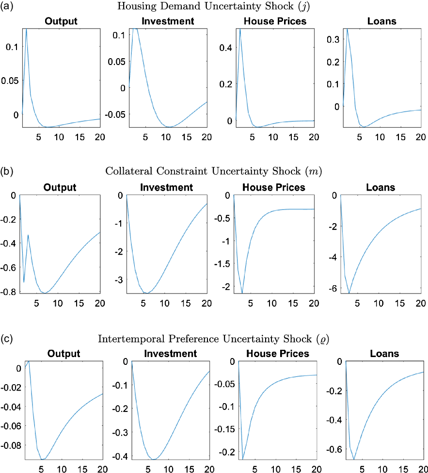
Figure 9. Responses of macroeconomic variables to uncertainty shocks.
Note: The figure plots the generalized impulse responses of selected variables to a one standard deviation increase in innovation of correspondent shocks. The responses are calculated at the unconditional mean of the states. All responses are normalized so that the units of the vertical axis are percentage deviations from the steady-state.
Almost all uncertainty shocks have negative effects on the output, house prices, and capital investment, showing the unfavorable economic conditions that high uncertainty creates. We investigate the transmission mechanisms of these shocks in more detail in Section 6.6, however, in general increases in uncertainty triggers precautionary savings, which reduces demand for consumption and housing. The precautionary saving motive also leads to an increase in labor supply but the positive effects of this increase are almost always outweighed by the negative impact of the precautionary savings. The economy particularly reacts to uncertainty in the financial sector through collateral constraints, while uncertainty about intertemporal preferences and housing demand have smaller but important effects on the economy.
A positive uncertainty shock for housing demand is an exception among the uncertainty shocks since it actually has a positive effect on output, as shown in Figure 9a. The housing demand uncertainty directly affects the utility that households receive from housing services. When there is housing demand uncertainty, households do not know if they will receive higher or lower utility from housing services, therefore the precautionary saving motive is not triggered. In particular, households would not decrease their consumption today to save more if they have low utility from housing services. If they have high utility, they would buy more housing now which would increase house prices, starting a positive spillover due to the collateral channel. Moreover, entrepreneurs do not face a similar uncertainty since they do not receive utility from housing services. If the households have high utility, then house prices would increase which would increase their collateral value as well. But if the households have lower utility, then house prices would decrease which would be a good time to invest in housing for entrepreneurs as it is used in production. Overall, entrepreneurs buy more housing regardless of the outcome of the housing uncertainty shock, which increases the house prices, creating the positive spillover in the economy.
On the other hand, an increase in uncertainty about collateral constraints raises concerns about how much households will be able to borrow in the future. As a result, households decrease their consumption due to a precautionary saving motive, as can be seen in Figure 9b. Lower credit availability combined with the direct effects of collateral uncertainty leads to a reduction in borrowing, and therefore, a reduction in demand for and the price of housing. Low house prices decrease the collateral value, which lowers investment by entrepreneurs. All of these changes result in a decrease in output.
An intertemporal preference uncertainty shock, as shown in Figure 9c, creates uncertainty about future consumption, which leads to precautionary savings. As households save more instead of investing in housing, house prices decrease. Lower consumption and house prices along with lack of credit availability lead to a decrease in output, loans, and investment.
6.6 Transmission mechanisms of uncertainty shocks
In this section, we investigate the transmission mechanisms of uncertainty shocks in more detail. In particular, we compare impulse responses to uncertainty shocks under different calibrations for the credit channel, adjustment costs, and monetary policy.
6.6.1 The role of the credit channel
The first set of alternative GIRFs shown in Figure 10 helps us understand the role of the credit channel in transmitting uncertainty shocks to the economy. Responses are calibrated with lax collateral constraints, where we set the LTV ratio higher than the benchmark model. In particular, the blue line shows the responses of output, investment, house prices, and total loans, when the LTV ratio is 0.79 (benchmark) and the black dashed line represents the case in which LTV is equal to 0.9 (lax credit conditions). Higher LTV ratios result in better access to credit because borrowers can use a larger fraction of their house value as collateral.
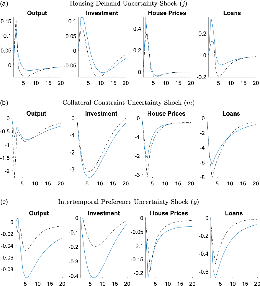
Figure 10. Responses of macroeconomic variables to uncertainty shocks under different LTVs.
Note: The figure plots the generalized impulse responses of selected variables to a one standard deviation increase in innovation of correspondent shocks. The responses are calculated at the unconditional mean of the states. The black, dashed line is calculated with the LTV ratio, $m=0.9$
, whereas the blue line shows the benchmark case where
$m=0.9$
, whereas the blue line shows the benchmark case where $m=0.79$
. All responses are normalized so that the units of the vertical axis are percentage deviations from the steady-state.
$m=0.79$
. All responses are normalized so that the units of the vertical axis are percentage deviations from the steady-state.
As Figure 10a shows, when there are lax credit conditions, the effects of housing demand uncertainty decrease for investment, house prices, and loans while increasing the response of output. The output response increases under lax credit conditions because of an increase in consumption. When borrowers have better credit access, they do not need to worry as much about the uncertainty or take strict precautionary actions. They can cope with the negative effects by borrowing in the future as they have better access to credit, which leads to an increase in their consumption. Although there are significant increases in the consumption of entrepreneurs and constrained households, there is not much change in the consumption of unconstrained households, as they are not subject to borrowing constraints. Lax credit conditions also mute the effects of the changes in the collateral value, which decreases the responses in other macroeconomic aggregates. For instance, the high LTV ratio makes the gains from increases in house prices smaller and offsets the negative effects from a decrease in house prices.
Figure 10b shows that the responses to uncertainty about the tightness of the collateral constraints have a more pronounced effect on output when access to credit is better. Under good credit access, constrained households become highly levered and more susceptible to the tightness of the collateral constraint. Therefore, uncertainty about collateral constraints leads to bigger decreases in consumption and housing services purchased by constrained households due to the precautionary saving motive. As the housing demand decreases, so do house prices and output, leading to larger changes compared to normal credit conditions. While entrepreneurs are also affected by the uncertainty, the differing levels of LTV do not significantly change the path of investment.
As can be seen in Figure 10c, increasing the LTV level dampens the effects of the intertemporal preference uncertainty shock. This result is due to the looser credit conditions reducing the need to worry about precautionary savings. Therefore, the demand reduces less, which results in smaller changes to all variables of interest.
6.6.2 The role of adjustment costs
The counterfactuals in this section aim to show the role of adjustment costs in promoting the effects of uncertainty in the economy. In particular, the GIRFs are calibrated with no housing adjustment costs in Figure 11 and with no capital adjustment costs in Figure 12.
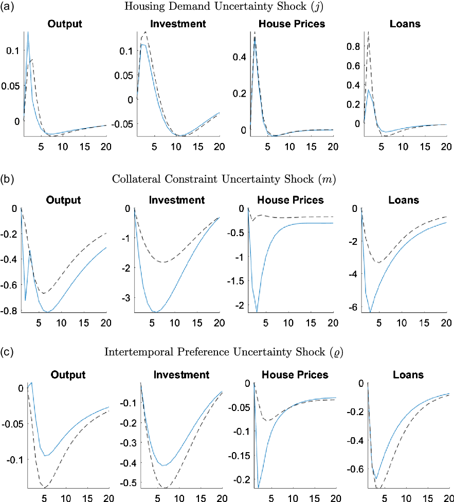
Figure 11. Responses of macroeconomic variables to uncertainty shocks without housing adjustment costs.
Note: The figure plots the generalized impulse responses of selected variables to a one standard deviation increase in innovation of correspondent shocks. The black, dashed line is calculated with $\psi _h = 0$
and the blue line shows the benchmark case where
$\psi _h = 0$
and the blue line shows the benchmark case where $\psi _h = 0.096$
. The responses are calculated at the unconditional mean of the states. All responses are normalized so that the units of the vertical axis are percentage deviations from the steady-state.
$\psi _h = 0.096$
. The responses are calculated at the unconditional mean of the states. All responses are normalized so that the units of the vertical axis are percentage deviations from the steady-state.
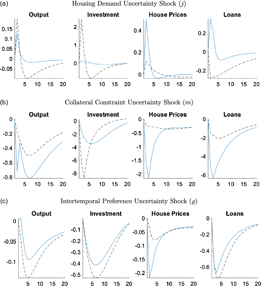
Figure 12. Responses of macroeconomic variables to uncertainty shocks without capital adjustment costs.
Note: The figure plots the generalized impulse responses of selected variables to a one standard deviation increase in innovation of correspondent shocks. The black, dashed line is calculated with $\psi _k = 0$
and the blue line shows the benchmark case where
$\psi _k = 0$
and the blue line shows the benchmark case where $\psi _k = 4.403$
. The responses are calculated at the unconditional mean of the states. All responses are normalized so that the units of the vertical axis are percentage deviations from the steady-state.
$\psi _k = 4.403$
. The responses are calculated at the unconditional mean of the states. All responses are normalized so that the units of the vertical axis are percentage deviations from the steady-state.
Figure 11 compares the case in which it is costless for households and entrepreneurs to change their housing stock ( $\psi _h = 0$
) to the benchmark case (
$\psi _h = 0$
) to the benchmark case ( $\psi _h = 0.096$
), which is calibrated at the posterior mode. As Figure 11b shows, the removal of the housing adjustment cost particularly dampens the effects of the collateral constraint uncertainty shock. An increase in collateral constraint uncertainty increases the risk entrepreneurs face of not being able to borrow as much as they would like the next period, which can lead to changes in their housing stock. However, when the housing adjustment costs are zero, it becomes less of a concern as changing the housing stock to cope with the negative effects of uncertainty is costless. The removal of the housing adjustment cost has a negligible effect on the responses to the housing demand uncertainty, however, it magnifies the effects of intertemporal preference uncertainty. This amplification arises from the larger decrease in investment. Since there are still capital adjustment costs, housing becomes less risky for entrepreneurs. Therefore, they substitute away from capital to housing, which reduces investment. However, the increase of the housing demand by entrepreneurs is offset by the decrease in housing demand by the households, which leads to an overall decrease in house prices at the end. Depressed house prices combined with low investment results in a decrease in output in the economy.
$\psi _h = 0.096$
), which is calibrated at the posterior mode. As Figure 11b shows, the removal of the housing adjustment cost particularly dampens the effects of the collateral constraint uncertainty shock. An increase in collateral constraint uncertainty increases the risk entrepreneurs face of not being able to borrow as much as they would like the next period, which can lead to changes in their housing stock. However, when the housing adjustment costs are zero, it becomes less of a concern as changing the housing stock to cope with the negative effects of uncertainty is costless. The removal of the housing adjustment cost has a negligible effect on the responses to the housing demand uncertainty, however, it magnifies the effects of intertemporal preference uncertainty. This amplification arises from the larger decrease in investment. Since there are still capital adjustment costs, housing becomes less risky for entrepreneurs. Therefore, they substitute away from capital to housing, which reduces investment. However, the increase of the housing demand by entrepreneurs is offset by the decrease in housing demand by the households, which leads to an overall decrease in house prices at the end. Depressed house prices combined with low investment results in a decrease in output in the economy.
The next alternative GIRFs in Figure 12 are calibrated with no capital adjustment costs, $\psi _k=0$
, making it costless for entrepreneurs to change their level of capital investment. The absence of capital adjustment costs allows entrepreneurs to quickly adjust their capital stock in response to an uncertainty shock. This ability leads to a large increase in investment after a housing demand uncertainty shock, as entrepreneurs substitute away from housing to capital. As can be seen in Figure 12a, the housing uncertainty shock still has a positive effect on house prices, as described in Section 6.5.2 even when the capital adjustment costs are removed. However, compared to the benchmark case, such positive effects are much smaller. Overall, the increases in both investment and house prices lead to an expansion in output.
$\psi _k=0$
, making it costless for entrepreneurs to change their level of capital investment. The absence of capital adjustment costs allows entrepreneurs to quickly adjust their capital stock in response to an uncertainty shock. This ability leads to a large increase in investment after a housing demand uncertainty shock, as entrepreneurs substitute away from housing to capital. As can be seen in Figure 12a, the housing uncertainty shock still has a positive effect on house prices, as described in Section 6.5.2 even when the capital adjustment costs are removed. However, compared to the benchmark case, such positive effects are much smaller. Overall, the increases in both investment and house prices lead to an expansion in output.
The absence of capital adjustment costs results in smaller changes to output for the uncertainty shock to collateral constraints, as can be seen in Figure 12b. Entrepreneurial demand for housing and capital declines in response to these uncertainty shocks. In the counterfactual GIRF, it is costless for them to adjust their capital stock but costly to adjust housing. Therefore, their demand for housing stays stable while they greatly reduce their investment. Stable house prices allow constrained households to still borrow since their collateral value has not changed significantly. Because they can continue to borrow, uncertainty shocks have a smaller affect on consumption, which also results in a smaller decline in output.
The interetemporal preference uncertainty shock causes larger declines in output and investment when there are no capital adjustment shocks, as can be seen in Figure 12c. Similar to the collateral constraint uncertainty shock, the intertemporal preference uncertainty shock reduces entrepreneurial demand for housing and capital. Since entrepreneurs can freely adjust their capital holdings, they change their housing demand less, stabilizing house prices. However, uncertainty about intertemporal preferences also directly affects demand for households, as they are not sure about their future consumption decisions. Therefore, the smaller decline in house prices is not enough to stabilize consumption and offset the bigger decline in investment, which results in a bigger decrease in output.
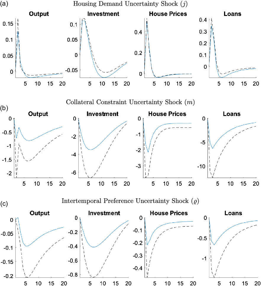
Figure 13. Responses of macroeconomic variables to uncertainty shocks with passive monetary policy.
Note: The figure plots the generalized impulse responses of selected variables to a one standard deviation increase in innovation of correspondent shocks. The black, dashed line is calculated with $\psi _\Pi = 2.2$
and
$\psi _\Pi = 2.2$
and $\psi _Y=0.35$
and the blue line shows the benchmark case where
$\psi _Y=0.35$
and the blue line shows the benchmark case where $\psi _\Pi = 4.45$
and
$\psi _\Pi = 4.45$
and $\psi _Y=0.71$
. The responses are calculated at the unconditional mean of the states. All responses are normalized so that the units of the vertical axis are percentage deviations from the steady-state.
$\psi _Y=0.71$
. The responses are calculated at the unconditional mean of the states. All responses are normalized so that the units of the vertical axis are percentage deviations from the steady-state.
6.6.3 The role of monetary policy
In this section, we try to understand the role of monetary policy in the transmission mechanism of uncertainty shocks by comparing a more passive monetary policy to our benchmark model. This counterfactual gives a glimpse into the potential effects of reaching the zero lower bound.
The GIRFs in Figure 13 are calibrated so that in the passive monetary policy the reaction to inflation is 2.2 and to output is 0.35 (black dashed line) which are then compared to the benchmark (blue line) where the inflation reaction is 4.45 and output reaction is 0.71 following the posterior modes of our estimation.
Monetary policy does not have a significant effect on the GIRFs for the housing demand uncertainty shock; however, it amplifies all the macroeconomic responses to the collateral and intertemporal preference uncertainty shocks. As expected, a passive monetary policy cannot guard the economy against negative impacts of uncertainty shocks effectively, decreasing output and inflation. Given that the interest rates do not fall by as much, output and investment decrease even further. These negative effects spill over to the housing and financial sector simultaneously, causing a credit crunch and low house prices, and therefore, deepening the recession.
7. Conclusion
This paper analyzes the importance of stochastic volatility and its role in the economy in a setting that allows for time-varying volatility in house prices. We first show that house prices have significant time-varying volatility by using rolling standard deviations of house prices, estimating a stochastic volatility reduced form model, and analyzing the underlying states of the stochastic volatility shock to house prices. We then estimate a DSGE model with housing, financial frictions, and stochastic volatility using a nonlinear approximation and Bayesian econometric techniques.
Our results confirm the importance of the housing market in generating and amplifying the economic activity. In particular, any level or uncertainty shock that causes an increase in the house prices generates a positive spillover to the economy through the financial sector. On the other hand, uncertainty, regardless of which market it comes from, provokes recessions in general. The results also highlight the importance of financial frictions in amplifying uncertainty shocks. We find that uncertainty about financial conditions has economically important effects. These findings complement the empirical research that has stressed the importance of financial uncertainty (Caldara et al. (Reference Caldara, Fuentes-Albero, Gilchrist and Zakrajšek2016), Ludvigson et al. (Reference Ludvigson, Ma and Ng2021)) and the theoretical literature considering other types of financial frictions (Christiano et al. (Reference Christiano, Motto and Rostagno2014), Higgins (Reference Higgins2023)).
We also show that stochastic volatility shocks improve model fit and contribute to generating house price volatility. In fact, stochastic volatility shocks create almost half of the house price volatility during the Great Recession. The three most important uncertainty shocks that affect the economy are the stochastic volatility shocks to collateral constraints, housing demand, and intertemporal preferences. For instance, collateral constraint uncertainty raises concerns about how much households will be able to borrow in the future which triggers precautionary savings. A decrease in the demand, in return, lowers house prices, making collateral constraints tighter for everyone. Adverse credit conditions cause a negative feedback loop in the economy, which decreases output. These negative effects on macroeconomic variables range between 1 and 6%. Moreover, we find that credit conditions, adjustment costs of capital and housing, and monetary policy seem to be important transmission mechanisms for the uncertainty shocks.
Supplementary material
To view supplementary material for this article, please visit https://doi.org/10.1017/S136510052300010X.
Acknowledgements
A previous version circulated as “House Price Uncertainty.” We wish to thank Dean Scrimgeour, Nicole Simpson and participants at the Utah Macro Workshop (Utah State University, 2019) and the Workshop in Macroeconomic Research at Liberal Arts Colleges (Macalester College, 2019) for comments. Richard Higgins would like to thank the Colgate Faculty Research Council for financial support.
Conflicts of interest
None.
A. Appendix
A.1 GARCH estimation
In this section, we estimate an AR(1)/GARCH(1,1) model using the house price growth data. GARCH(1,1) model is commonly used in the literature to analyze high volatility time series data (for instance, Cunningham (Reference Cunningham2006), Han (Reference Han2010, Reference Han2013), among others). The model allows the conditional variance of house prices to depend on the past realizations of the error process while modeling the time dependent mean and variance.
Table A1. AR(1)/GARCH(1,1) house price growth
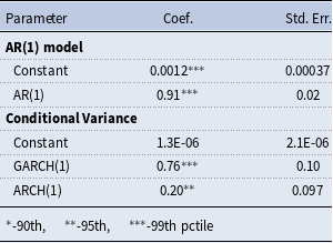
Note: The optimal lags are chosen by the Akaike and Bayesian information criteria.
The results are presented in Table A1 showing that the AR(1) process is heteroskedastic. The estimated coefficients of ARCH and GARCH terms are significant, suggesting that the volatility of house prices change over time. Moreover, the sum of these two terms are close to one which indicates covariance stationary model with a high degree of persistence and long memory of conditional variance. The GARCH term is greater than the ARCH term which shows that the old information on house price changes are very important for the current and future house prices which is consistent from the evidence of Case and Shiller (Reference Case and Shiller1988). The AR(1)/GARCH(1,1) was picked by both Akaike (AIC) and Bayesian (BIC) information criteria over several competing models. These values can be seen in Table A2.
Table A2. GARCH estimation: information criteria
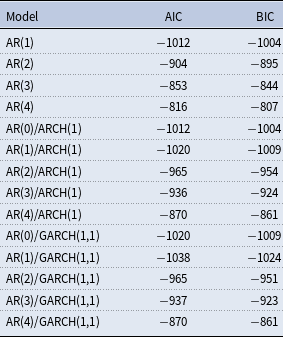
A.2 The role of the Great Recession on house price volatility
The Great Recession, which was caused by a housing bust, was a significant source of house price volatility. Therefore, it is important to understand whether time-varying volatility that we observe in data is driven by that period. To study the role of this period and show the existence of the house price volatility in other time periods, we first exclude the Great Recession in Figure 1. Removing the high uncertainty period due to the Great Recession makes it easier to see the time-variation in the standard deviation for the earlier periods. As can bee seen from Figure A1, there is still a significant variation in the volatility of house prices even when the Great Recession is excluded. Despite being lower in magnitude than the Great Recession, early and late 90s still exhibit sharp increases in house price volatility.
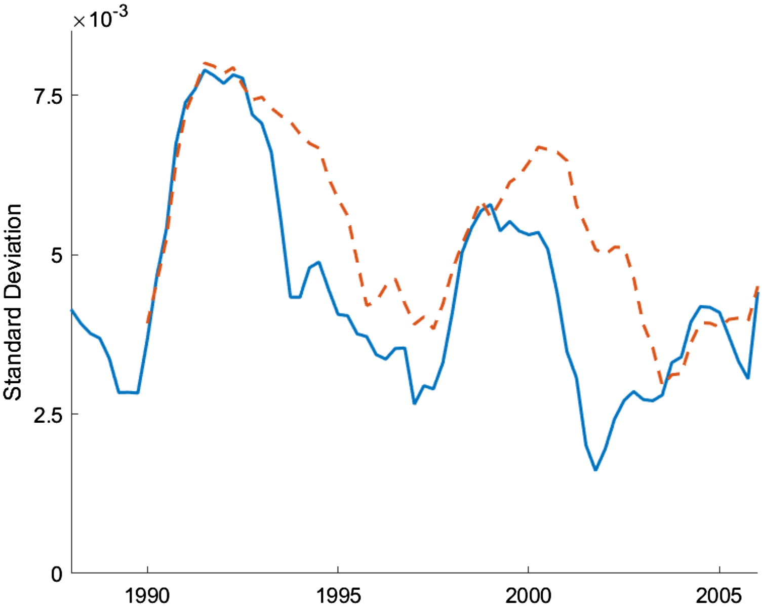
Figure A1. Rolling standard deviations of house price growth.
Note: The figure plots 4-yr (solid, blue line) and 6-yr (dashed, orange line) rolling standard deviations of house price growth which is defined as the log differences in the quarterly averages of monthly fannie mac house price. The data are seasonally adjusted and deflated by the GDP deflator.
To understand whether time-varying volatility is driven by the Great Recession more formally, we consider three specifications. First, we run the reduced-form regression with the sample ending in 2007Q4, at the start of the Great Recession. Second, we allow for a structural break starting in 2007Q4 in the steady state standard deviation. The final specification allows for the steady state standard deviation to change from 2007Q4 to 2010Q4 (this differs from the previous specification since the model reverts back to the original steady state standard deviation in 2011Q1). If the time-varying volatility only picks up changes in volatility due to the Great Recession, these exercises will greatly reduce the importance of stochastic volatility.
The results from the estimates of the alternative specifications are presented in two tables. The posterior mode under different specifications can be seen in Table A3. The results are similar both quantitatively and qualitatively to the results from the baseline estimation of the paper. Table A4 shows the log marginal data density (MDD) of the reduced form estimates. The inclusion of stochastic volatility greatly improves model fit in all specifications.
The underlying state of the time-varying standard deviation from the reduced form estimates can be seen in Figure A2. Each specification shows very similar results to those from the baseline specification from the paper. Overall, we can conclude that while the Great Recession is an important source of variation in house prices, it is not the only period where prices exhibit time-varying volatility. House price volatility seems to persist even after we control for the Great Recession.
A.3 First order conditions of the model
A.3.1 Entrepreneurs
The optimization problem of entrepreneurs yields the following first order conditions where $g_{I}$
is the growth rate of investment,
$g_{I}$
is the growth rate of investment, $\lambda _t$
,
$\lambda _t$
, $\lambda _{b,t}$
, and
$\lambda _{b,t}$
, and $\lambda _{k,t}$
are the Lagrangian multipliers for the flow of funds, borrowing constraint, and the law of capital motion, respectively.
$\lambda _{k,t}$
are the Lagrangian multipliers for the flow of funds, borrowing constraint, and the law of capital motion, respectively.
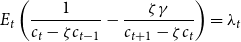 \begin{equation} E_t\left ( \frac{1}{c_{t}-\zeta c_{t-1}}-\frac{\zeta \gamma }{c_{t+1}-\zeta c_{t}}\right ) =\lambda _{t} \end{equation}
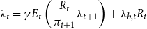 \begin{equation} \lambda _{t}=\gamma E_{t}\left ( \frac{R_{t}}{\pi _{t+1}}\lambda _{t+1}\right ) +\lambda _{b,t}R_{t} \end{equation}
Table A3. Prior and posterior distribution: alternative reduced form estimates
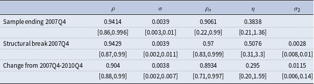
Note: 95% credible set centered around the median is quoted underneath the posterior mode.
Table A4. Model fit: reduced form estimate
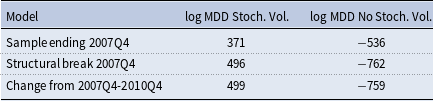
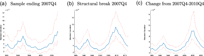
Figure A2. Underlying states: alternative reduced form estimation.
Note: Smoothed underlying states are calculated at the posterior mode and are transformed to show the standard deviation of the innovation to the level shock. The median filtered states are shown along with the 5th and 95th percentiles.
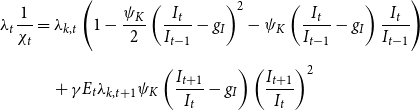 \begin{align} \lambda _{t}\frac{1}{\chi _{t}}&=\lambda _{k,t}\left ( 1-\frac{\psi _{K}}{2}\left ( \frac{I_{t}}{I_{t-1}}-g_{I}\right ) ^{2}-\psi _{K}\left ( \frac{I_{t}}{I_{t-1}}-g_{I}\right ) \frac{I_{t}}{I_{t-1}}\right )\nonumber \\[5pt] & \quad +\gamma E_t\lambda _{k,t+1}\psi _{K}\left ( \frac{I_{t+1}}{I_{t}}-g_{I}\right ) \left ( \frac{I_{t+1}}{I_{t}}\right ) ^{2} \end{align}
 \begin{equation} E_t\left\{\lambda _{t}\gamma \frac{\mu Y_{t+1}}{X_{t+1}K_{t}}+\lambda _{b,t}m_{t}u_{t+1}\pi _{t+1}-\lambda _{k,t}+\lambda _{k,t+1}\gamma (1-\delta )\right\}=0 \end{equation}
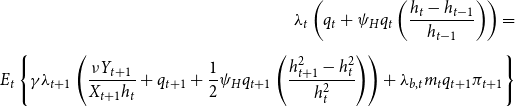 \begin{equation} \begin{split} \lambda _{t}\left ( q_{t}+\psi _{H}q_{t}\left ( \frac{h_{t}-h_{t-1}}{h_{t-1}}\right ) \right ) =\\[5pt] E_t\left \{ \gamma \lambda _{t+1}\left ( \frac{\nu Y_{t+1}}{X_{t+1}h_{t}}+q_{t+1}+\frac{1}{2}\psi _{H}q_{t+1}\left ( \frac{h_{t+1}^{2}-h_{t}^{2}}{h_{t}^{2}}\right ) \right ) +\lambda _{b,t}m_{t}q_{t+1}\pi _{t+1}\right \} \end{split} \end{equation}
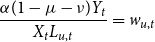 \begin{equation} \frac{\alpha (1-\mu -\nu )Y_{t}}{X_{t}L_{u,t}}=w_{u,t} \end{equation}
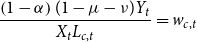 \begin{equation} \frac{\left ( 1-\alpha \right ) (1-\mu -\nu )Y_{t}}{X_{t}L_{c,t}}=w_{c,t} \end{equation}
A.3.2 Unconstrained households
The optimization problem for the unconstrained households yields the following first order conditions.
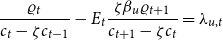 \begin{equation} \frac{\varrho _{t}}{c_{t}-\zeta c_{t-1}}-E_t\frac{\zeta \beta _u\varrho _{t+1}}{c_{t+1}-\zeta c_{t}}=\lambda _{u,t} \end{equation}
 \begin{equation} \lambda _{u,t}-E_t\beta _u\lambda _{u,t+1}\frac{R_{t}}{\pi _{t+1}}=0 \end{equation}
 \begin{equation} \lambda _{u,t}\left ( q_{t}+\psi _{u,H}q_{t}\frac{h_{u,t}-h_{u,t-1}}{h_{u,t-1}}\right ) =\varrho _{t}\frac{j_u}{h_{u,t}}+E_t\beta _u \lambda _{u,t+1}\left ( \frac{\psi _{u,H}q_{t+1}}{2}\left ( \frac{h_{u,t+1}^{2}-h_{u,t}^{2 }}{h_{u,t}^{2}}\right ) +q_{t+1}\right ) \end{equation}
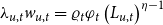 \begin{equation} \lambda _{u,t}w_{u,t}=\varrho _{t}\varphi _{t}\left ( L_{u,t}\right ) ^{\eta -1} \end{equation}
where $\lambda _{u,t}$
is the Lagrangian multiplier of the budget constraint.
$\lambda _{u,t}$
is the Lagrangian multiplier of the budget constraint.
A.3.3 Constrained households
The first order conditions to the optimization problem of constrained households are as follows:
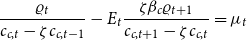 \begin{equation} \frac{\varrho _{t}}{c_{c,t}-\zeta c_{c,t-1}}-E_t\frac{\zeta \beta _c\varrho _{t+1}}{c_{c,t+1}-\zeta c_{c,t}}=\mu _{t} \end{equation}
 \begin{equation} \mu _{t}-E_t\beta _c \mu _{t+1}\frac{R_{t}}{\pi _{t+1}}-\lambda _{c,t}R_{t}=0 \end{equation}
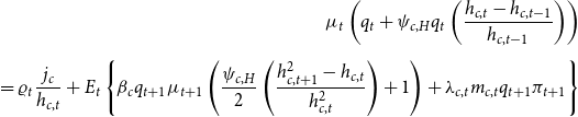 \begin{equation} \begin{split} \mu _{t}\left ( q_{t}+\psi _{c,H}q_{t}\left ( \frac{h_{c,t}-h_{c,t-1}}{h_{c,t-1}}\right ) \right ) \\[5pt] =\varrho _{t}\frac{j_c}{h_{c,t}}+E_{t}\left \{ \beta _cq_{t+1}\mu _{t+1}\left ( \frac{\psi _{c,H}}{2}\left ( \frac{h_{c,t+1}^{2}-h_{c,t}}{h_{c,t}^{2}}\right ) +1\right ) +\lambda _{c,t}m_{c,t}q_{t+1}\pi _{t+1}\right \} \end{split} \end{equation}
 \begin{equation} w_{c,t}\mu _{t}=\varrho _{t}\varphi _{t}\left ( L_{c,t}\right ) ^{\eta _c -1} \end{equation}
where $\lambda _{c,t}$
and
$\lambda _{c,t}$
and $\mu _{t}$
are Lagrangian multipliers for the budget constraint and borrowing constraint, respectively.
$\mu _{t}$
are Lagrangian multipliers for the budget constraint and borrowing constraint, respectively.
A.3.4 Retailers
The optimization problem yields the demand curve in equation (53) as well as equations (54)–(56).
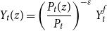 \begin{equation} Y_{t}(z)=\left ( \frac{P_{t}(z)}{P_{t}}\right ) ^{-\varepsilon }Y_{t}^{f} \end{equation}
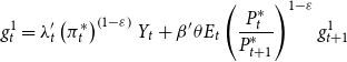 \begin{equation} g_{t}^{1}=\lambda _{t}^{\prime }\left ( \pi _{t}^{\ast }\right ) ^{\left ( 1-\varepsilon \right ) }Y_{t}+\beta ^{\prime }\theta E_{t}\left ( \frac{P_{t}^{\ast }}{P_{t+1}^{\ast }}\right ) ^{1-\varepsilon }g_{t+1}^{1} \end{equation}
 \begin{equation} g_{t}^{2}=\lambda _{t}^{\prime }\left ( \pi _{t}^{\ast }\right ) ^{-\varepsilon }\frac{Y_{t}}{X_{t}}+\beta ^{\prime }\theta E_{t}\left ( \frac{P_{t}^{\ast }}{P_{t+1}^{\ast }}\right ) ^{-\varepsilon }g_{t+1}^{2} \end{equation}
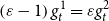 \begin{equation} \left ( \varepsilon -1\right ) g_{t}^{1}=\varepsilon g_{t}^{2} \end{equation}
A.4 Data
Data are obtained from NIPA-BEA, CPS-BLS, the FRED database, and the Flow of Funds accounts from the Federal Reserve Board for the period of 1984:Q1 to 2017:Q1. The following list documents the data used in the paper.
• Real output: quarterly real GDP divided by the civilian non-institutional population aged 16 and over from the BLS. It is log differenced from the quarter before.
• Real investment: the sum of personal consumption expenditures of durables, gross private domestic investment minus private fixed investment of residential and nonresidential structures deflated by their associated deflators (gross private domestic investment implicit price deflator, private fixed investment of residential implicit price deflator, private fixed investment of nonresidential structures implicit price deflator). It is divided by the civilian non-institutional population aged 16 and over from the BLS and is log differenced from the quarter before.
• Real consumption: the sum of personal consumption expenditures of non-durables and services deflated by their associated deflators. It is divided by the civilian non-institutional population aged 16 and over from the BLS and is log differenced from the quarter before.
• Hours: hours of all persons from the non-farm business sector divided by the non-institutional population aged 16 and over from the BLS. We take the log and demean the data.
• Inflation: the log difference (period t vs. t-1) of the GDP deflator.
• Federal funds rate: data are from the FRED database and are converted to quarterly rates using the average rate for each quarter.
• House prices: the quarterly average of the monthly Freddie Mac House Price Index which are seasonally adjusted and divided by the GDP deflator. It is log differenced from the quarter before.
A.5 Impulse responses
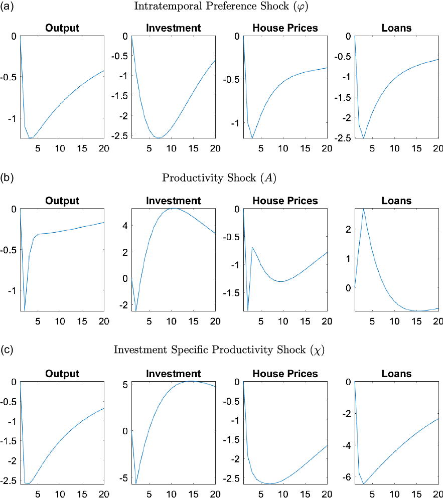
Figure A3. Responses of macroeconomic variables to other level shocks.
Note: The figure plots the generalized impulse responses of selected variables to a one standard deviation increase in innovation of correspondent shocks. The responses are calculated at the unconditional mean of the states. All responses are normalized so that the units of the vertical axis are percentage deviations from the steady-state. Output and investment are normalized by $A$
and
$A$
and $\chi$
, so they show increases when
$\chi$
, so they show increases when $A$
and
$A$
and $\chi$
are shocked, despite the levels increasing.
$\chi$
are shocked, despite the levels increasing.
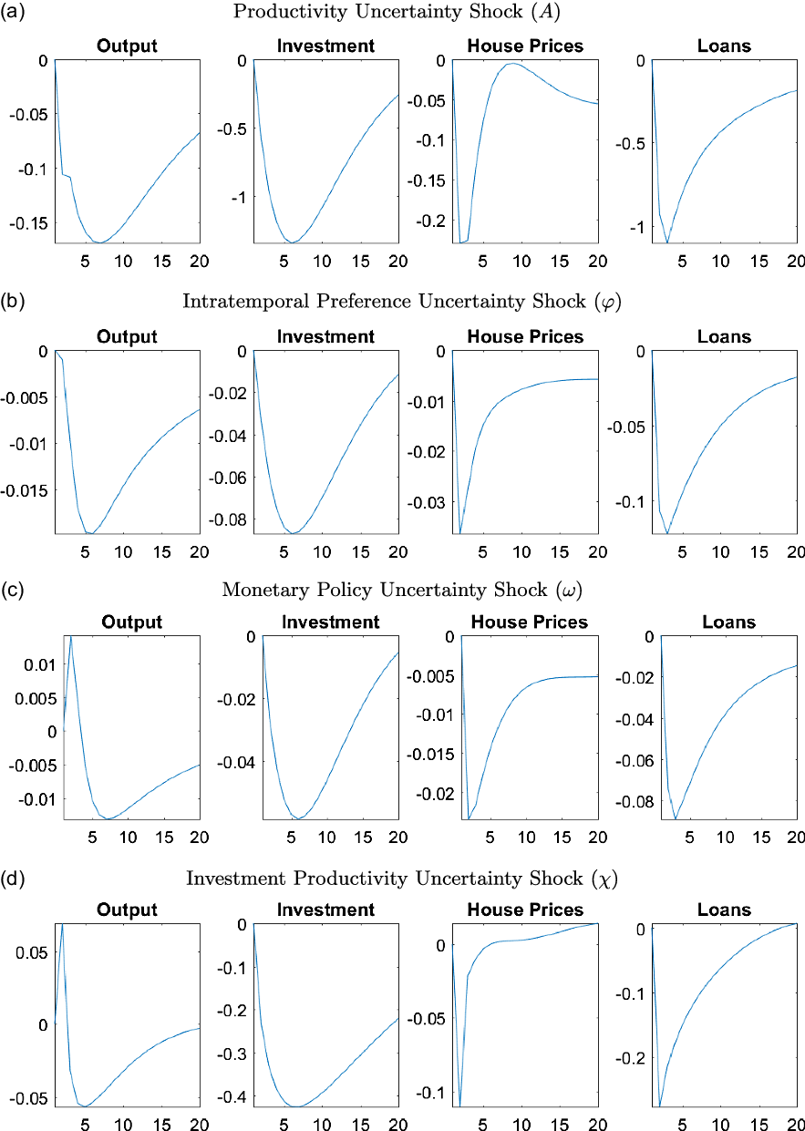
Figure A4. Responses of macroeconomic variables to other uncertainty shocks.
Note: The figure plots the generalized impulse responses of selected variables to a one standard deviation increase in innovation of correspondent shocks. The responses are calculated at the unconditional mean of the states. All responses are normalized so that the units of the vertical axis are percentage deviations from the steady-state.


