


1. Introduction
Although macroeconomic models with financial frictions were major workhorses in business cycle studies even before the 2008–2009 global financial crisis, most of them focused on the role of financial frictions only in propagating and amplifying shocks originating in firms’ productivity, households’ preferences, or economic policies. After the crisis, some studies shed light on the shocks affecting agents’ ability to borrow as a key influence on business cycles. Shocks to financial constraints are referred to as “financial shocks,” of which there are two main classes: a credit crunch that affects agents’ borrowing capacity (Jermann and Quadrini (Reference Jermann and Quadrini2012), Kahn and Thomas (Reference Kahn and Thomas2013), Buera and Moll (Reference Buera and Moll2015)), and a liquidity shortage that affects agents’ ability to issue and resell equity (Shi (Reference Shi2015), Kiyotaki and Moore (Reference Kiyotaki and Moore2019)). These theoretical studies show that adverse financial shocks induce a fall in GDP, aggregate consumption, investment, and employment.
Despite their successful explanation of realistic co-movements among major macroeconomic variables, some researchers have criticized these models. In particular, Shi (Reference Shi2015) points out that an adverse financial shock in such models, be it a credit crunch or a liquidity shortage, induces a rise in stock prices. Obviously, this theoretical prediction is not consistent with observations; instead, the opposite is true. Fig. 1 plots the movements of the GDP per capita and stock prices in the US before and after the 2008–2009 financial crisis.Footnote 1 As this figure shows, their movements are quite synchronized. As Shi (Reference Shi2015) notes, this problem is important and must be addressed, because a fall in stock prices is thought to be the prime transmission channel of financial shocks to the aggregate economy.
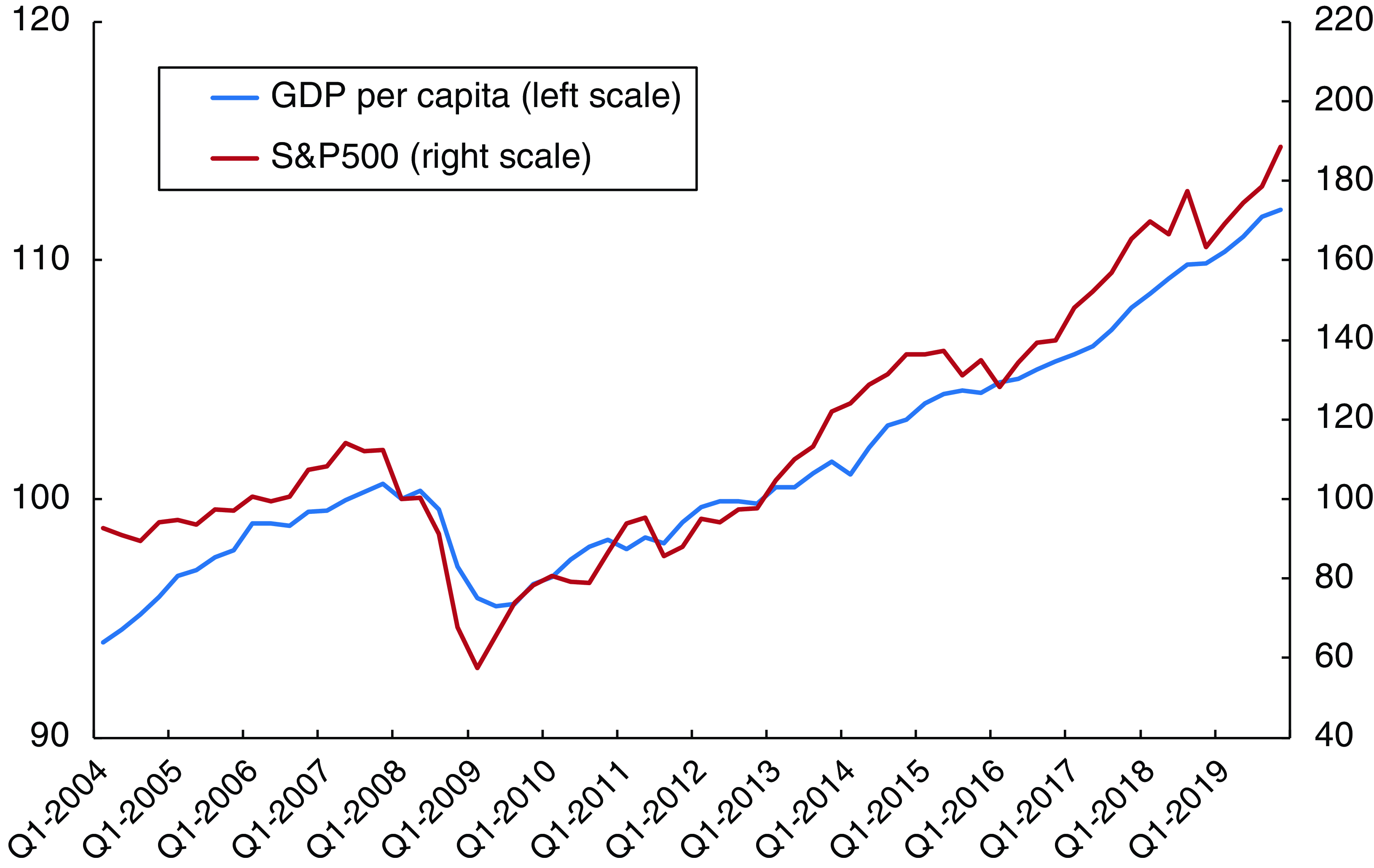
Figure 1. GDP per capita and the stock prices in the US.
How can we resolve this problem? Several studies have addressed this issue. Among others, using numerical analysis, Guerron-Quintana and Jinnai (Reference Guerron-Quintana and Jinnai2022) show that connecting a financial shock and endogenous growth can resolve the problem of the counterfactual stock price movement. They build on Shi (Reference Shi2015) and Kiyotaki and Moore (Reference Kiyotaki and Moore2019). Household members are classified into workers and entrepreneurs who accumulate physical capital through investment. Entrepreneurs can sell their own capital to finance investments, but there is an upper limit to the amount of capital that can be sold in one period. This creates a liquidity constraint for entrepreneurs, which in turn generates an upper limit on the amount of investments.
In their model, a negative financial shock is formulated so that the liquidity constraint becomes tighter and entrepreneurs become more cash-strapped. Because of such a shock, entrepreneurs’ capital investment decreases. This itself has the effect of raising the stock price of capital.Footnote 2 However, if technological progress is determined by learning-by-doing externalities à la Romer (Reference Romer1986), that is, labor productivity improves as the capital stock increases, then a decline in investment also has the additional effect of a subsequent deterioration in labor productivity. This deterioration in future productivity is then reflected in stock prices at the time of the shock, and thus, the financial shock causes a decline in stock prices. By using an endogenous growth model, they also succeeded in providing a theoretical explanation for why temporary negative financial shocks have lasting effects on the real economy.
However, the relationship between financial shocks and stock prices still needs to be analyzed for the following two reasons. First, Guerron-Quintana and Jinnai (Reference Guerron-Quintana and Jinnai2022) do not explicitly introduce a financial intermediary sector, such as banks, into their model. As seen with the bankruptcy of Lehman Brothers, the event triggering the financial crisis is often a negative shock to the banking sector. Therefore, it is important to introduce banks explicitly into the model and then analyze the stock price reaction to shocks affecting the banking sector. Second, they employ learning-by-doing externalities as the mechanism for endogenous growth. Indeed, by doing so they succeed in making the model concise. However, firms’ R&D activities are thought to be the main source of economic growth, as first stressed by Romer (Reference Romer1990), Grossman and Helpman (Reference Grossman and Helpman1991a), Aghion and Howitt (Reference Aghion and Howitt1992), and so on. Although Guerron-Quintana and Jinnai (Reference Guerron-Quintana and Jinnai2022) note that their results would be robust to the use of R&D-based endogenous growth models, they did not conduct this type of analysis. Therefore, the mechanism of how financial shocks affect R&D activities remains unclear. Fig. 2 illustrates how R&D spending in the US has evolved over time.Footnote 3 Over the ten years from 1998 to 2008, R&D spending grew at an annual rate of 3.6%. In this figure, the dashed line represents the counterfactual amount of spending if this growth rate had continued after 2008. As can be seen from this figure, R&D spending was below this counterfactual trend after 2008 until it recovered in 2021. Thus, the financial crisis has had a negative impact on R&D investment, and it is important to explicitly incorporate R&D activities into the model.

Figure 2. R&D spending in the US.
Against this background, this study examines the impacts of financial shocks to the banking sector on stock prices and the real economy by incorporating the banking sector into an R&D-based endogenous growth model. I formulate the banking sector in the same way as Gertler et al. (Reference Gertler, Kiyotaki and Prestipino2020).Footnote 4 I mainly consider the quality ladder developed by Grossman and Helpman (Reference Grossman and Helpman1991a, Reference Grossman and Helpman1991b: Ch.4) as the mechanism for endogenous growth. In the model, households make deposits, entrant firms issue equities to conduct R&D activities, and banks intermediate financial funds between them. This study adopts the following two key features of banks in Gertler et al. (Reference Gertler, Kiyotaki and Prestipino2020). First, although the households can purchase equities directly, banks are more efficient in doing so. Specifically, there is a utility cost for the households directly holding equities. Second, each bank has an incentive to divert its assets for its own use. This potential moral hazard leads to a situation in which the banks’ capacity to collect deposits is limited, and they face an upper bound of their leverage ratio. Based on the presence of this upper bound, in equilibrium, both households and banks purchase equities.
In the present model, a negative financial shock is formulated so that the moral hazard problem becomes more serious and the banks’ leverage ratio decreases. Within this framework, I analytically examine the long-run effects of this financial shock when it is permanent and numerically investigate the short-run and long-run effects when it is temporary.Footnote 5 In both cases, it is shown that such a shock causes both a prolonged downward shift in real activity and a sharp decline in stock prices. The mechanism generating this result is simple and can be explained as follows. After the shock, banks face more difficulty financing their equity investments with external funds due to a reduction in their leverage ratio. Banks are, however, better at equity investment. In such a case, the household is burdened by managing more firms and, therefore, demands a high premium to hold additional equities. This is achieved through a decrease in stock acquisition costs, that is, a reduction in stock price. The decline in stock prices then makes innovation less profitable for entrants, which in turn reduces R&D activities in the economy as a whole. In the endogenous growth model, R&D is the key determinant of the growth rate (i.e. future levels) of real variables. Thus, even if the financial shock is temporary and the resulting decline in R&D is also temporary, it will have a lasting negative impact on the level of real variables. As I have explained, the mechanism that generates this result is quite different from that in Guerron-Quintana and Jinnai (Reference Guerron-Quintana and Jinnai2022). In this sense, this study complements their analysis.
This study is related to several previous studies in addition to the literature cited so far. Ajello (Reference Ajello2016) and Del Negro et al. (Reference Del Negro, Eggertsson, Ferrero and Kiyotaki2017) incorporate both nominal price and wage rigidities into the model of Kiyotaki and Moore (Reference Kiyotaki and Moore2019) and argue that such nominal frictions are important to overcoming the problem of counterfactual stock price response. By contrast, this study does not require such rigidities. I believe that the solution they propose and the one presented in this study are complementary to each other. Because of its simplicity, the proposed mechanism in this study could easily be incorporated into their model. This study is also related to the literature linking business cycles to economic growth, such as Comin and Gertler (Reference Comin and Gertler2006), Kobayashi and Shirai (Reference Kobayashi and Shirai2018), Bianchi et al. (Reference Bianchi, Kung and Morales2019), Guerron-Quintana and Jinnai (Reference Guerron-Quintana and Jinnai2019), and Ikeda and Kurozumi (Reference Ikeda and Kurozumi2019), in the sense that they pursue business cycle implications in an R&D-based endogenous growth model. They build on quantitative dynamic stochastic general equilibrium models and explore the impacts of several economic shocks on the economy. By comparison, the goal of this study is to develop a tractable macroeconomic model and examine the relationships among financial shocks, R&D investments, and firms’ stock prices. One strength of the model proposed here is its tractability, which allows us to easily characterize the equilibrium and conduct comparative statics. The tractability can provide insight into the inner workings of the model when considering the effects of financial shocks.
The rest of this paper is organized as follows. Section 2 sets up the model. Section 3 analytically characterizes the equilibrium and provides the comparative statics. Section 4 presents the numerical results of a transitory financial shock to banks. Section 5 provides further discussion. Section 6 concludes the paper.
2. Model
Time is discrete and extends from zero to infinity ( $t=0, 1, 2, \dots$
). The supply side is a discrete-time version of a quality-ladder growth model developed by Grossman and Helpman (Reference Grossman and Helpman1991a, Reference Grossman and Helpman1991b: Ch.4).Footnote
6
The economy has a single final good used for consumption. There is one primary factor, labor, which is used for production of intermediate goods and R&D activities. Households save their income in the form of deposits at banks and direct claims on equities; however, they are less efficient in the direct claims than are banks. The banks intermediate funds between the households and the firms.
$t=0, 1, 2, \dots$
). The supply side is a discrete-time version of a quality-ladder growth model developed by Grossman and Helpman (Reference Grossman and Helpman1991a, Reference Grossman and Helpman1991b: Ch.4).Footnote
6
The economy has a single final good used for consumption. There is one primary factor, labor, which is used for production of intermediate goods and R&D activities. Households save their income in the form of deposits at banks and direct claims on equities; however, they are less efficient in the direct claims than are banks. The banks intermediate funds between the households and the firms.
2.1. Firms
Final good sector. The final good is a composite of differentiated intermediate goods indexed by $\omega \in [0, 1]$
. The production technology is given by
$\omega \in [0, 1]$
. The production technology is given by
 \begin{equation*} Y_t= Z_t \exp \left [ \int _0^1 \ln \left ( \lambda ^{K_t(\omega )} x_t(\omega ) \right ) d\omega \right ]\! , \end{equation*}
where $Y_t$
is the output of the final good,
$Y_t$
is the output of the final good, $x_t(\omega )$
is the demand for variety
$x_t(\omega )$
is the demand for variety $\omega$
,
$\omega$
, $K_t(\omega ) (\!=1, 2, \ldots )$
represents the highest quality of variety
$K_t(\omega ) (\!=1, 2, \ldots )$
represents the highest quality of variety $\omega$
in period
$\omega$
in period $t$
, and
$t$
, and $\lambda \gt 1$
represents the size of the quality improvement achieved by an innovation. Without loss of generality, I assume the initial condition
$\lambda \gt 1$
represents the size of the quality improvement achieved by an innovation. Without loss of generality, I assume the initial condition $K_0(\omega )=1$
for all
$K_0(\omega )=1$
for all $\omega$
. Then,
$\omega$
. Then, $K_t(\omega )-1$
is the number of occurrences of quality-upgrading innovations for
$K_t(\omega )-1$
is the number of occurrences of quality-upgrading innovations for $\omega$
before period
$\omega$
before period $t$
. The term
$t$
. The term $Z_t$
is the exogenous technology level, growing at a constant rate of
$Z_t$
is the exogenous technology level, growing at a constant rate of $g_Z\gt 0$
. Even if this term were not present, the qualitative results would not change at all. I introduce the term
$g_Z\gt 0$
. Even if this term were not present, the qualitative results would not change at all. I introduce the term $Z_t$
to capture the fact that there are other contributing factors to productivity growth in addition to R&D activities.Footnote
7
$Z_t$
to capture the fact that there are other contributing factors to productivity growth in addition to R&D activities.Footnote
7
Following Grossman and Helpman (Reference Grossman and Helpman1991b, Ch.4), I take the final expenditure as the numeraire: $P_t Y_t=1$
, where
$P_t Y_t=1$
, where $P_t$
is the price of the final good. Thus, in this model, all prices are evaluated in terms of the final expenditure. Let
$P_t$
is the price of the final good. Thus, in this model, all prices are evaluated in terms of the final expenditure. Let $p_t(\omega )$
denote the price of variety
$p_t(\omega )$
denote the price of variety $\omega$
. Profit maximization yields the demand function for variety
$\omega$
. Profit maximization yields the demand function for variety $\omega$
:
$\omega$
: $ x_t(\omega )=1/p_t(\omega )$
and the zero-profit condition:
$ x_t(\omega )=1/p_t(\omega )$
and the zero-profit condition:
 \begin{equation} P_t= \dfrac{1}{Z_t} \exp \left [ \int _0^1 \ln \left ( \dfrac{p_t(\omega )}{ \lambda ^{K_t(\omega )}} \right )d\omega \right ]\!. \end{equation}
Intermediate good sector. Producing $x_t(\omega )$
units requires the same units of labor as inputs, implying that the wage rate
$x_t(\omega )$
units requires the same units of labor as inputs, implying that the wage rate $W_t$
is the unit cost of production. As in Grossman and Helpman (Reference Grossman and Helpman1991a, Reference Grossman and Helpman1991b: Ch.4), each variety has several potential suppliers that can produce the good with a quality of less than
$W_t$
is the unit cost of production. As in Grossman and Helpman (Reference Grossman and Helpman1991a, Reference Grossman and Helpman1991b: Ch.4), each variety has several potential suppliers that can produce the good with a quality of less than $K_t(\omega )$
. The leader firm determines its price as
$K_t(\omega )$
. The leader firm determines its price as $p_t( \omega ) =\lambda W_t$
to monopolize the market, and it sells
$p_t( \omega ) =\lambda W_t$
to monopolize the market, and it sells $x_t(\omega ) = 1/ (\lambda W_t)$
units of the good. The resulting profit is
$x_t(\omega ) = 1/ (\lambda W_t)$
units of the good. The resulting profit is $\pi _t(\omega )=\pi \equiv 1-1/\lambda$
.
$\pi _t(\omega )=\pi \equiv 1-1/\lambda$
.
Let $Q_t$
denote the end-of-period stock price of the leader firm. Here, “end-of-period” has two meanings. First,
$Q_t$
denote the end-of-period stock price of the leader firm. Here, “end-of-period” has two meanings. First, $Q_t$
is ex-dividend, that is,
$Q_t$
is ex-dividend, that is, $Q_t$
is evaluated after the dividend in period
$Q_t$
is evaluated after the dividend in period $t$
has been paid. Second,
$t$
has been paid. Second, $Q_t$
is evaluated after it turns out that the innovation did not occur in period
$Q_t$
is evaluated after it turns out that the innovation did not occur in period $t$
.Footnote
8
Let
$t$
.Footnote
8
Let $R^e_{t+1}$
denote the one-period gross rate of return from holding the equity from the end of period
$R^e_{t+1}$
denote the one-period gross rate of return from holding the equity from the end of period $t$
to
$t$
to $t+1$
.
$t+1$
.
 \begin{equation} R^e_{t+1} \equiv \dfrac{\pi +(1-I_{t+1})Q_{t+1} }{Q_t}, \end{equation}
where $I_{t+1} \in [0, 1]$
denotes the probability that an innovation by potential entrants succeeds in period
$I_{t+1} \in [0, 1]$
denotes the probability that an innovation by potential entrants succeeds in period $t+1$
and the current leader loses its market power.
$t+1$
and the current leader loses its market power. $I_t$
is determined endogenously from the resource constraint in this economy. As in the literature on quality-ladder growth,
$I_t$
is determined endogenously from the resource constraint in this economy. As in the literature on quality-ladder growth, $I_t$
is independent and identically distributed (i.i.d.) across varieties. Then, from the law of large numbers,
$I_t$
is independent and identically distributed (i.i.d.) across varieties. Then, from the law of large numbers, $I_t$
is equal to the ex-post measure of varieties in which innovation occurs.
$I_t$
is equal to the ex-post measure of varieties in which innovation occurs.
If each potential entrant hires $\kappa I_t$
units of labor in period
$\kappa I_t$
units of labor in period $t$
, then it can succeed in innovation with probability
$t$
, then it can succeed in innovation with probability $I_t$
, where
$I_t$
, where $\kappa \gt 1$
is the labor requirement to obtain 100% success in innovation. If the innovation succeeds, then the entrant becomes the new leader firm for one variety from period
$\kappa \gt 1$
is the labor requirement to obtain 100% success in innovation. If the innovation succeeds, then the entrant becomes the new leader firm for one variety from period $t+1$
. Consequently, the new leader faces the idiosyncratic risk of the next innovation and other aggregate risks. Therefore, the expected benefit of innovation in period
$t+1$
. Consequently, the new leader faces the idiosyncratic risk of the next innovation and other aggregate risks. Therefore, the expected benefit of innovation in period $t$
is given by
$t$
is given by $I_t Q_t$
. Then, the free entry condition of R&D activities for a variety is
$I_t Q_t$
. Then, the free entry condition of R&D activities for a variety is $Q_t \leq W_t \kappa$
, the equality of which holds if
$Q_t \leq W_t \kappa$
, the equality of which holds if $I_t\gt 0$
, that is, R&D is conducted. Throughout this study, I focus on the equilibrium with
$I_t\gt 0$
, that is, R&D is conducted. Throughout this study, I focus on the equilibrium with $I_t \gt 0$
.
$I_t \gt 0$
.
 \begin{equation} Q_t= W_t \kappa. \end{equation}
2.2. Households
I formulate this sector in a similar way as Gertler et al. (Reference Gertler, Kiyotaki and Prestipino2020). There is a continuum of households, and each household in turn consists of a continuum of family members with measure $1+f\gt 0$
, where
$1+f\gt 0$
, where $f\in (0, 1)$
is constant. Within a household, members are classified into workers and bankers. The measure of workers is 1, while that of bankers is
$f\in (0, 1)$
is constant. Within a household, members are classified into workers and bankers. The measure of workers is 1, while that of bankers is $f$
. I normalize the measure of households to 1 so that the total population is constant at
$f$
. I normalize the measure of households to 1 so that the total population is constant at $1+f$
.Footnote
9
Each worker supplies labor to earn wages, and each banker manages a bank. The detail of the bankers’ behavior is explained in Section 2.3.
$1+f$
.Footnote
9
Each worker supplies labor to earn wages, and each banker manages a bank. The detail of the bankers’ behavior is explained in Section 2.3.
As seen in Section 2.1, the measure of profit-earning intermediate good firms is unity. Let $S^h_t$
be the number of firms whose equities are held directly by the households and
$S^h_t$
be the number of firms whose equities are held directly by the households and $S^b_t$
be the number of firms whose equities are intermediated by the bankers. Then,
$S^b_t$
be the number of firms whose equities are intermediated by the bankers. Then,
 \begin{equation*} S^h_t+S^b_t=1. \end{equation*}
Within the household, the members consume the same amount of the final good. Let $C_t$
denote the amount of aggregate real consumption. Each member consumes
$C_t$
denote the amount of aggregate real consumption. Each member consumes $C_t/(1+f)$
. Each worker is endowed with one unit of time. Since the population of workers is normalized to 1,
$C_t/(1+f)$
. Each worker is endowed with one unit of time. Since the population of workers is normalized to 1, $L_t$
also represents the total labor supply. The representative household’s utility is given byFootnote
10
$L_t$
also represents the total labor supply. The representative household’s utility is given byFootnote
10
 \begin{equation*} E_0 \left \{ \sum _{t=0}^\infty \beta ^t \Big [ \ln C_t + \zeta \ln\! (1-L_t) - \Gamma \big(S^h_t\big) \Big ] \right \}\! , \end{equation*}
where $\beta \in (0, 1)$
is the discount factor,
$\beta \in (0, 1)$
is the discount factor, $ \zeta \gt 0$
is the weight of the utility from leisure, and
$ \zeta \gt 0$
is the weight of the utility from leisure, and $ E_t(\!\cdot\! )$
is the expectation operator conditioned on the information available in period
$ E_t(\!\cdot\! )$
is the expectation operator conditioned on the information available in period $t$
. Function
$t$
. Function $\Gamma$
represents the disutility from the household’s direct equity holding. Following Gertler et al. (Reference Gertler, Kiyotaki and Prestipino2020), I introduce this disutility function to simply capture the household’s lower efficiency in handling equity investments compared to banks.Footnote
11
I assume that function
$\Gamma$
represents the disutility from the household’s direct equity holding. Following Gertler et al. (Reference Gertler, Kiyotaki and Prestipino2020), I introduce this disutility function to simply capture the household’s lower efficiency in handling equity investments compared to banks.Footnote
11
I assume that function $\Gamma$
satisfies
$\Gamma$
satisfies
 \begin{equation*} \Gamma ^{\prime}(S^h)\gt 0, \Gamma ^{\prime\prime}(S^h)\gt 0 \text { for } S^h\gt 0, \Gamma ^{\prime}(0) = 0. \end{equation*}
By the law of large numbers, the fraction $I_t$
of the leader firms are leapfrogged at the end of period
$I_t$
of the leader firms are leapfrogged at the end of period $t$
; the stock price of these firms then becomes zero. As in the existing studies employing the quality-ladder growth model, I assume that the household can diversify equity investments. Thus, the households are not exposed to any risk other than the aggregate financial shocks that we will see in Section 2.3. Therefore, the budget constraint is given byFootnote
12
$t$
; the stock price of these firms then becomes zero. As in the existing studies employing the quality-ladder growth model, I assume that the household can diversify equity investments. Thus, the households are not exposed to any risk other than the aggregate financial shocks that we will see in Section 2.3. Therefore, the budget constraint is given byFootnote
12
 \begin{equation*} R^d_t D_{t-1}+R^e_t Q_{t-1} S^h_{t-1} +W_t L_t +\Pi ^{bank}_t -T_t = P_t C_t +D_t +Q_t S^h_t , \end{equation*}
where $D_t$
represents deposits,
$D_t$
represents deposits, $R^d_t$
is the gross rate of return on the deposits,
$R^d_t$
is the gross rate of return on the deposits, $T_t$
represents lump-sum taxes, and
$T_t$
represents lump-sum taxes, and $\Pi ^{bank}_t$
shows the transfers from bankers; how
$\Pi ^{bank}_t$
shows the transfers from bankers; how $\Pi ^{bank}_t$
is determined is explained in Section 2.3.
$\Pi ^{bank}_t$
is determined is explained in Section 2.3.
The household chooses $C_t, L_t, S^h_t$
, and
$C_t, L_t, S^h_t$
, and $D_t$
to maximize the utility subject to the budget constraint. The conditions for utility maximization are given by
$D_t$
to maximize the utility subject to the budget constraint. The conditions for utility maximization are given by
 \begin{align*} &\dfrac{\zeta }{ 1-L_t}=\dfrac{W_t}{P_t C_t},\\ &\dfrac{1}{P_t C_t}=\beta E_t \left (\dfrac{1}{P_{t+1}C_{t+1}} R^d_{t+1}\right )\!, \\ &\dfrac{\Gamma ^{\prime}\big(S^h_t\big)}{Q_t}+\dfrac{1}{P_t C_t}= \beta E_t \left ( \dfrac{1}{P_{t+1} C_{t+1} } R^e_{t+1} \right )\!. \end{align*}
Since the market equilibrium of the final good implies $P_tC_t=P_t Y_t (\!=1)$
, these conditions can be rewritten as
$P_tC_t=P_t Y_t (\!=1)$
, these conditions can be rewritten as
 \begin{align} &L_t = 1-\dfrac{\zeta }{W_t}, \end{align}
 \begin{align} &E_t R^d_{t+1} =\dfrac{1}{\beta }, \end{align}
 \begin{align} &E_t \!\left ( R^e_{t+1}-R^d_{t+1} \right )= \dfrac{\Gamma ^{\prime}\big(S^h_t\big)}{\beta Q_t}. \end{align}
2.3. Banks
Each banker manages a bank. Hereafter, I use bankers and banks interchangeably. The aggregate net revenue of bankers in period $t$
is given by
$t$
is given by $R^e_t Q_{t-1}S^b_{t-1}-R^d_t D_{t-1}$
. At the end of each period, each banker faces an idiosyncratic risk of exit that occurs with probability
$R^e_t Q_{t-1}S^b_{t-1}-R^d_t D_{t-1}$
. At the end of each period, each banker faces an idiosyncratic risk of exit that occurs with probability $1-\delta \in (0, 1)$
. Throughout this study, I assume the following inequality:
$1-\delta \in (0, 1)$
. Throughout this study, I assume the following inequality:
Assumption 1. $\delta \lt \beta .$
Each bank, if it is hit by the exit shock, gives its net revenue to the household. Since the exit probability is i.i.d. across bankers, the $1-\delta$
share of the aggregate net revenue is transferred to the household:
$1-\delta$
share of the aggregate net revenue is transferred to the household:
 \begin{equation*} \Pi ^{bank}_t= (1-\delta )\big(R^e_t Q_{t-1}S^b_{t-1}-R^d_t D_{t-1}\big). \end{equation*}
After exiting, a banker becomes a worker starting in the next period. To keep the populations of both workers and bankers constant over time, the workers with mass $(1-\delta )f \in (0, 1)$
are randomly chosen at the end of each period to act as bankers starting in the next period.
$(1-\delta )f \in (0, 1)$
are randomly chosen at the end of each period to act as bankers starting in the next period.
Consider a bank with its net revenue given by $n_t = R^e_t Q_{t-1} s^b_{t-1} -R^d_t d_{t-1}$
, where
$n_t = R^e_t Q_{t-1} s^b_{t-1} -R^d_t d_{t-1}$
, where $s^b_{t-1}$
is the measure of firms purchased by this bank and
$s^b_{t-1}$
is the measure of firms purchased by this bank and $d_{t-1}$
is the issued deposits. If this bank is not hit by the exit shock, it then finances equity purchases
$d_{t-1}$
is the issued deposits. If this bank is not hit by the exit shock, it then finances equity purchases $Q_t s^b_t$
with this revenue and newly issued deposits:
$Q_t s^b_t$
with this revenue and newly issued deposits:
 \begin{equation} Q_t s^b_t=n_t+d_t. \end{equation}
Then, this bank’s net revenue in period $t+1$
is given by
$t+1$
is given by $n_{t+1}=R^e_{t+1}Q_t s^b_t -R^d_{t+1} d_t$
. Note that (7) represents the banker’s balance sheet and
$n_{t+1}=R^e_{t+1}Q_t s^b_t -R^d_{t+1} d_t$
. Note that (7) represents the banker’s balance sheet and $n_t$
corresponds to the banker’s net worth. Henceforth, I simply call
$n_t$
corresponds to the banker’s net worth. Henceforth, I simply call $n_t$
net worth. In Appendix A.1, it is shown that the banker’s objective function is given by
$n_t$
net worth. In Appendix A.1, it is shown that the banker’s objective function is given by
 \begin{equation*} \tilde V_t \equiv E_t\! \left \{\sum _{j=1}^\infty \beta ^j (1-\delta ) \delta ^{j-1} n_{t+j} \right \}\!. \end{equation*}
The term $(1-\delta )\delta ^{j-1}$
is the conditional probability of exit in period
$(1-\delta )\delta ^{j-1}$
is the conditional probability of exit in period $t+j$
given that the bank does not exit in period
$t+j$
given that the bank does not exit in period $t$
. Let
$t$
. Let $V_t(n_t) \equiv \max \tilde V_t$
denote the value function. The banker’s optimization problem is written as the Bellman equation:
$V_t(n_t) \equiv \max \tilde V_t$
denote the value function. The banker’s optimization problem is written as the Bellman equation:
 \begin{align*} V_t(n_t)=\max _{s^b_t, d_t} E_t \big \{ \beta \big [(1-\delta )n_{t+1}+\delta V_{t+1}(n_{t+1}) \big ] \big \}. \end{align*}
The bank faces the balance sheet condition (7) and the following constraint:
 \begin{equation} \widetilde V_t \geq \theta _t Q_t s^b_t, \end{equation}
which comes from the potential moral hazard problem. After buying equities, the bank has the following two options. One is to hold the assets, receive dividends, and then meet its deposit obligations in period $t+1$
. The other is to secretly sell the assets to obtain the funds for its own use. To remain undetected, the bank can sell only up to fraction
$t+1$
. The other is to secretly sell the assets to obtain the funds for its own use. To remain undetected, the bank can sell only up to fraction $\theta _t$
of the assets. Inequality (8) is a constraint in which the bank has no incentive to choose the latter option. In this model, a change in
$\theta _t$
of the assets. Inequality (8) is a constraint in which the bank has no incentive to choose the latter option. In this model, a change in $\theta _t$
generates a financial shock.
$\theta _t$
generates a financial shock. $\theta _t$
changes according to
$\theta _t$
changes according to
 \begin{equation*} \ln\! (\theta _{t+1}/\theta )=\rho \ln\! (\theta _t/\theta )+\varepsilon _{t+1}, \end{equation*}
where $\theta$
is the baseline value of
$\theta$
is the baseline value of $\theta _t$
,
$\theta _t$
, $\varepsilon _t$
is an i.i.d. shock, and
$\varepsilon _t$
is an i.i.d. shock, and $\rho \in (0, 1)$
is the parameter specifying the persistence of shocks.
$\rho \in (0, 1)$
is the parameter specifying the persistence of shocks.
To solve the problem, we can use the guess and verify method. Guess $V_t(n_t)$
as a linear function of
$V_t(n_t)$
as a linear function of $n_t$
:
$n_t$
: $V_t(n_t)=\psi _t n_t$
. The Bellman equation is rewritten as
$V_t(n_t)=\psi _t n_t$
. The Bellman equation is rewritten as
 \begin{equation*} \psi _t n_t = E_t \left \{ \beta (1-\delta +\delta \psi _{t+1}) \max _{s^b_t} \left [ R^d_{t+1} n_t + \left (R^e_{t+1}-R^d_{t+1}\right )Q_t s^b_t\right ] \right \}, \end{equation*}
subject to $\psi _t n_t \geq \theta _t Q_t s^b_t.$
Then, as long as
$\psi _t n_t \geq \theta _t Q_t s^b_t.$
Then, as long as $R^e_{t+1}-R^d_{t+1}\gt 0$
, the bank invests as much as it can:
$R^e_{t+1}-R^d_{t+1}\gt 0$
, the bank invests as much as it can:
 \begin{equation} Q_t s^b_t = \dfrac{\psi _t n_t}{\theta _t}. \end{equation}
Substituting this result into the Bellman equation yields the dynamic equation of $\psi _t$
:
$\psi _t$
:
 \begin{align} \psi _t= \dfrac{ \beta E_t\! \left [ (1-\delta +\delta \psi _{t+1} ) R^d_{t+1} \right ]}{\left \{ 1- \frac{\beta }{\theta _t} E_t\left [ (1-\delta +\delta \psi _{t+1} ) \left (R^e_{t+1}-R^d_{t+1}\right ) \right ] \right \} }. \end{align}
The denominator is assumed to be positive:
Assumption 2. $\theta _t \gt \beta E_t \left [ (1-\delta +\delta \psi _{t+1} ) \left (R^e_{t+1}-R^d_{t+1}\right ) \right ]$
.
$\theta _t \gt \beta E_t \left [ (1-\delta +\delta \psi _{t+1} ) \left (R^e_{t+1}-R^d_{t+1}\right ) \right ]$
.
Consider a banker that newly enters the market. Let $e_t$
denote the new banker’s initial net worth and assume that this is fully subsidized by the government. The new banker’s behavior is then given by (7) and (9), with
$e_t$
denote the new banker’s initial net worth and assume that this is fully subsidized by the government. The new banker’s behavior is then given by (7) and (9), with $n_t$
replaced by
$n_t$
replaced by $e_t$
. The same equation as (10) is then implied for the new banker. Let
$e_t$
. The same equation as (10) is then implied for the new banker. Let $N$
denote the aggregate net worth of banks. To obtain the equilibrium of the model, I assume that the subsidies to each new banker are proportional to the average net worth in the previous period. Since the measure of bankers is always
$N$
denote the aggregate net worth of banks. To obtain the equilibrium of the model, I assume that the subsidies to each new banker are proportional to the average net worth in the previous period. Since the measure of bankers is always $f$
,
$f$
,
 \begin{equation*} e_t= \mu N_{t-1}/f, \end{equation*}
where I assume that $\mu \gt 0$
is not so large:
$\mu \gt 0$
is not so large:
Assumption 3. $\mu \lt \frac{\beta -\delta }{\beta (1-\delta )} (\!\lt 1)$
.
$\mu \lt \frac{\beta -\delta }{\beta (1-\delta )} (\!\lt 1)$
.
This assumption is required to obtain the uniqueness of the equilibrium. $N_t$
is then given by the sum of the incumbent banks’ net worth as well as that of the new entrants:
$N_t$
is then given by the sum of the incumbent banks’ net worth as well as that of the new entrants:
 \begin{align*} N_t = \delta \big(R^e_t Q_{t-1} S^b_{t-1}-R^d_t D_{t-1}\big) + (1-\delta ) \mu N_{t-1}. \end{align*}
Since each bank’s decision about equity holding $Q_t s^b_t$
is linear in its state variable
$Q_t s^b_t$
is linear in its state variable $n_t$
or
$n_t$
or $e_t$
, these decisions are easily aggregated over all banks. Given
$e_t$
, these decisions are easily aggregated over all banks. Given $N_t$
,
$N_t$
, $Q_t S^b_t$
is given by
$Q_t S^b_t$
is given by
 \begin{equation*} Q_t S^b_t=\dfrac {\psi _t N_t}{\theta _t}. \end{equation*}
Thus, $\psi _t/\theta _t$
represents the banks’ leverage.
$\psi _t/\theta _t$
represents the banks’ leverage.
2.4. Government
The government’s budget constraint is given by
 \begin{equation*} T_t= (1-\delta ) \mu N_{t-1}, \end{equation*}
from which $T_t$
is determined.
$T_t$
is determined.
2.5. Market-clearing conditions
The timing of events during a given period is summarized as follows.
-
1. Aggregate financial shocks are realized. The workers determine their labor supply, the final and intermediate good firms produce the goods, and the intermediate good firms pay dividends to the equity owners.
-
2. The outcomes of R&D are realized. By the law of large numbers, the fraction $I_t$
of the leader firms is leapfrogged and the stock price of these firms becomes zero. Since the shareholders have diversified equity investments, their total values of equity change from
$Q_{t-1}S^{h(b)}_{t-1}$
to
$Q_t(1-I_t)S^{h(b)}_{t-1}$
. Their gross interest income from holding equities is
$\pi +Q_t(1-I_t)S^{h(b)}_{t-1} =R^e_t Q_{t-1}S^{h(b)}_{t-1}$
. In this stage, the households also obtain the gross interest income from their deposits,
$R^d_t D_{t-1}.$
$I_t$
of the leader firms is leapfrogged and the stock price of these firms becomes zero. Since the shareholders have diversified equity investments, their total values of equity change from
$Q_{t-1}S^{h(b)}_{t-1}$
to
$Q_t(1-I_t)S^{h(b)}_{t-1}$
. Their gross interest income from holding equities is
$\pi +Q_t(1-I_t)S^{h(b)}_{t-1} =R^e_t Q_{t-1}S^{h(b)}_{t-1}$
. In this stage, the households also obtain the gross interest income from their deposits,
$R^d_t D_{t-1}.$
-
3. Each bank exits in this stage with an i.i.d. probability of
$1-\delta \in (0, 1)$
. Upon exit, the profits of such banks,
$\Pi ^{bank}_t$
, are transferred to the households. The workers with mass
$(1-\delta )f$
become new bankers and enter the financial market with their initial net worth subsidized by the government. The households pay the lump-sum taxes
$T_t$
to the government. -
4. The asset markets open. The households consume the final good and determine their portfolios,
$Q_t S^h_t$
and
$D_t$
, respectively. The bankers buy the equities
$Q_t S^b_t.$


The market-clearing condition for the final good is $Y_t=C_t =1/P_t$
. The labor market clears as
$Y_t=C_t =1/P_t$
. The labor market clears as
 \begin{equation} L_t = \dfrac{1}{\lambda W_t}+\kappa I_t. \end{equation}
The market-clearing condition of equities is $S^h_t+S^b_t=1$
. Finally, the deposits
$S^h_t+S^b_t=1$
. Finally, the deposits $D_t$
must satisfy
$D_t$
must satisfy
 \begin{equation} D_t+N_t= Q_t S^b_t. \end{equation}
From these market-clearing conditions, together with the agents’ behavior, the household’s budget constraint is automatically satisfied from Walras’ law.
3. Equilibrium in the deterministic economy
This section analytically characterizes the equilibrium in the case of no aggregate risks by assuming $\varepsilon _t=0$
(i.e.
$\varepsilon _t=0$
(i.e. $\theta _t=\theta$
) for all
$\theta _t=\theta$
) for all $t$
. In this case, (5) and (6) are respectively reduced to
$t$
. In this case, (5) and (6) are respectively reduced to
 \begin{equation} R^d_{t+1}=1/\beta, \end{equation}
 \begin{equation} R^e_{t+1}= \dfrac{1}{\beta }\left (1+\dfrac{\Gamma ^{\prime}\big(S^h_t\big)}{ Q_t} \right ). \end{equation}
3.1. Equilibrium conditions
This subsection derives key equations in characterizing the equilibrium. Substituting (13) and (14) into (10) without the expectation operator yields
 \begin{equation} \psi _t = (1-\delta +\delta \psi _{t+1}) \left (1+ \dfrac{\psi _t}{\theta } \dfrac{\Gamma ^{\prime}\big(S^h_t\big)}{Q_t}\right ). \end{equation}
Substituting (12)–(14) and $Q_t S^b_t= \psi _t N_t/\theta$
into the banks’ aggregate net worth in period
$Q_t S^b_t= \psi _t N_t/\theta$
into the banks’ aggregate net worth in period $t+1$
, we can obtain the dynamic equation of
$t+1$
, we can obtain the dynamic equation of $N_t$
as follows:
$N_t$
as follows:
 \begin{equation} N_{t+1}= \left [ \dfrac{\delta }{\beta } \left (1+ \dfrac{\psi _t}{\theta }\dfrac{\Gamma ^{\prime}\big(S^h_t\big)}{Q_t}\right ) +(1-\delta )\mu \right ] N_t. \end{equation}
Substituting (3) and (4) into the labor market equilibrium (11) and evaluating the resulting equation in period $t+1$
,
$t+1$
,
 \begin{equation} I_{t+1}= \dfrac{1}{\kappa } -\dfrac{1+\lambda \zeta }{\lambda } \dfrac{1}{Q_{t+1}}. \end{equation}
Substituting (14) and (17) into (2), we can obtain the dynamic equation of $Q_t$
as follows:
$Q_t$
as follows:
 \begin{equation} Q_t=\beta (1-1/\kappa )Q_{t+1}+\beta (1+\zeta )-\Gamma ^{\prime}\big(S^h_t\big). \end{equation}
Equations (15), (16), and (18) include $S^h_t$
. Since
$S^h_t$
. Since $S^h_t +S^b=1$
,
$S^h_t +S^b=1$
, $S^h_t$
is given by the functions of
$S^h_t$
is given by the functions of $\psi _t$
,
$\psi _t$
, $N_t$
, and
$N_t$
, and $Q_t$
:
$Q_t$
:
 \begin{equation} S^h_t= 1- \dfrac{\psi _t N_t}{\theta Q_t}. \end{equation}
Thus, the autonomous dynamical system in the deterministic economy is given by (15), (16), and (18) together with (19). Note that $N_t$
is a state variable, whereas
$N_t$
is a state variable, whereas $\psi _t$
and
$\psi _t$
and $Q_t$
are forward-looking variables whose initial values are determined endogenously.
$Q_t$
are forward-looking variables whose initial values are determined endogenously.
3.2. Balanced growth path
In this section, I examine the equilibrium where $Q_t, \psi _t, N_t, S^h_t$
, and
$Q_t, \psi _t, N_t, S^h_t$
, and $I_t$
become stationary. I call such an equilibrium the balanced growth path (BGP) equilibrium, since in that case consumption grows at a constant rate as shown below.
$I_t$
become stationary. I call such an equilibrium the balanced growth path (BGP) equilibrium, since in that case consumption grows at a constant rate as shown below.
Equation (16) with $N_t=N_{t+1}$
implies
$N_t=N_{t+1}$
implies
 \begin{equation} 1+ \dfrac{\psi }{\theta }\dfrac{\Gamma ^{\prime}(S^h)}{Q}=B^\ast, \end{equation}
where
 \begin{equation*} B^\ast \equiv \dfrac {\beta [1-(1-\delta )\mu ]}{\delta }\gt 1. \end{equation*}
Note that $B^\ast$
depends only on the exogenous parameters and Assumption 3 ensures
$B^\ast$
depends only on the exogenous parameters and Assumption 3 ensures $B^\ast \gt 1$
. Hereafter, a superscript asterisk over a variable represents its stationary value. For example,
$B^\ast \gt 1$
. Hereafter, a superscript asterisk over a variable represents its stationary value. For example, $\psi ^*$
denotes the stationary value of
$\psi ^*$
denotes the stationary value of $\psi$
. Equation (15) with
$\psi$
. Equation (15) with $\psi _t=\psi _{t+1}$
provides
$\psi _t=\psi _{t+1}$
provides $\psi ^*$
:
$\psi ^*$
:
 \begin{equation*} \psi ^\ast =\dfrac {(1-\delta )B^\ast }{1-\delta B^\ast }\gt 0. \end{equation*}
Substituting the obtained $\psi ^\ast$
back into equation (20) yields the following relationship between the stock price
$\psi ^\ast$
back into equation (20) yields the following relationship between the stock price $Q$
and the households’ equity purchases
$Q$
and the households’ equity purchases $S^h$
:
$S^h$
:
 \begin{equation} Q = \dfrac{\delta \psi ^\ast }{\left [ \beta -\delta - \beta (1-\delta )\mu \right ] \theta }\Gamma ^{\prime}(S^h), \end{equation}
where the sign of the denominator is positive from Assumption 3. Since $\Gamma ^{\prime\prime}(S^h)\gt 0$
for
$\Gamma ^{\prime\prime}(S^h)\gt 0$
for $S^h\gt 0$
, this equation shows a positive relationship between
$S^h\gt 0$
, this equation shows a positive relationship between $q$
and
$q$
and $S^h$
. The intuition is explained as follows. When
$S^h$
. The intuition is explained as follows. When $S^h$
becomes larger, households become more reluctant to hold equities directly unless their rate of return becomes sufficiently higher. Indeed,
$S^h$
becomes larger, households become more reluctant to hold equities directly unless their rate of return becomes sufficiently higher. Indeed, $R^e-R^d=\Gamma ^{\prime}(S^h)/(\beta Q)$
experiences upward pressure. This upward pressure in turn has a positive impact on the banks’ aggregate net worth
$R^e-R^d=\Gamma ^{\prime}(S^h)/(\beta Q)$
experiences upward pressure. This upward pressure in turn has a positive impact on the banks’ aggregate net worth $N$
, and hence, they want to purchase more of these equities. In the stationary equilibrium in which
$N$
, and hence, they want to purchase more of these equities. In the stationary equilibrium in which $N$
is constant, such an increase in their equity demand puts upward pressure on the stock price
$N$
is constant, such an increase in their equity demand puts upward pressure on the stock price $Q$
. As equation (20) shows, the upward pressure on
$Q$
. As equation (20) shows, the upward pressure on $S^h$
is offset by a rise in
$S^h$
is offset by a rise in $Q$
such that
$Q$
such that $R^e-R^d$
remains constant.
$R^e-R^d$
remains constant.
There is the other relationship between $q$
and
$q$
and $S^h$
. From (18) with
$S^h$
. From (18) with $Q_t=Q_{t+1}$
, we can obtain
$Q_t=Q_{t+1}$
, we can obtain
 \begin{equation} Q= \dfrac{\beta (1+\zeta )-\Gamma ^{\prime}(S^h)}{1-\beta (1-1/\kappa )}, \end{equation}
where the sign of the denominator is positive. Since $\Gamma ^{\prime\prime}(S^h)\gt 0$
for
$\Gamma ^{\prime\prime}(S^h)\gt 0$
for $S^h\gt 0$
, this equation shows a negative relationship between
$S^h\gt 0$
, this equation shows a negative relationship between $q$
and
$q$
and $S^h$
. The intuition is straightforward. The increase in
$S^h$
. The intuition is straightforward. The increase in $S^h$
makes households less willing to hold equities unless their rate of return becomes sufficiently higher. Therefore, this unwillingness depresses the unit cost of the equity purchase, which is
$S^h$
makes households less willing to hold equities unless their rate of return becomes sufficiently higher. Therefore, this unwillingness depresses the unit cost of the equity purchase, which is $Q$
.
$Q$
.
In Fig. 3, the upward- and downward-sloping curves represent equations (21) and (22), respectively. These two curves have only one intersection. $Q^\ast$
is explicitly obtained as
$Q^\ast$
is explicitly obtained as
 \begin{equation*} Q^\ast = \dfrac { \beta (1+\zeta ) \delta \psi ^\ast }{[1-\beta (1-1/\kappa )]\delta \psi ^\ast + [\beta -\delta -\beta (1-\delta )\mu ]\theta }. \end{equation*}
By its definition, $S^{h*}$
must be in
$S^{h*}$
must be in $(0, 1)$
. Since I assume
$(0, 1)$
. Since I assume $\Gamma ^{\prime}(0)=0$
, the value of
$\Gamma ^{\prime}(0)=0$
, the value of $Q$
in (21) is necessarily smaller than
$Q$
in (21) is necessarily smaller than $Q$
in (22) for
$Q$
in (22) for $S^h=0.$
Thus,
$S^h=0.$
Thus, $S^{h*}\gt 0$
is guaranteed. Throughout this study, I also assume that
$S^{h*}\gt 0$
is guaranteed. Throughout this study, I also assume that $S^{h*}\lt 1$
is satisfied, and hence, equity holdings are diversified between banks and households. For example, given
$S^{h*}\lt 1$
is satisfied, and hence, equity holdings are diversified between banks and households. For example, given $Q^*$
,
$Q^*$
, $S^{h\ast }\lt 1$
is satisfied if
$S^{h\ast }\lt 1$
is satisfied if
 \begin{equation} \Gamma ^{\prime}(1)\gt \dfrac{Q^\ast }{\delta \psi ^\ast }[\beta -\delta -\beta (1-\delta )\mu ] \theta. \end{equation}
Substituting $Q_{t+1}=Q^*$
into (17) yields
$Q_{t+1}=Q^*$
into (17) yields $I^\ast$
:
$I^\ast$
:
 \begin{equation} I^\ast = \dfrac{1}{\kappa }-\dfrac{1+\lambda \zeta }{\lambda Q^\ast }. \end{equation}
By its definition, $I^*$
must be in (0, 1). Note that
$I^*$
must be in (0, 1). Note that $I^\ast \lt 1$
is guaranteed because of
$I^\ast \lt 1$
is guaranteed because of $\kappa \gt 1$
. From (24),
$\kappa \gt 1$
. From (24), $I^*\gt 0$
if and only if
$I^*\gt 0$
if and only if
 \begin{equation} Q^\ast \gt \dfrac{\kappa (1+\lambda \zeta )}{\lambda }. \end{equation}
The results obtained so far can be summarized as the following Proposition:

Figure 3. Determination of $S^{h*}$
and
$S^{h*}$
and $Q^*$
.
$Q^*$
.
Proposition 1. There exists a unique BGP equilibrium with a positive growth rate and diversification of equity holdings if (23) and (25) are satisfied.
Then, I derive the growth rate of consumption, which always grows at the same rate as the inverse of the final good price. Since $p_t(\omega )=\lambda W_t$
for all
$p_t(\omega )=\lambda W_t$
for all $\omega$
, equation (1) implies
$\omega$
, equation (1) implies
 \begin{equation*} P_t= \dfrac {W_t} {(1+g_Z)^t \lambda ^{\int _0^1 (K_t(\omega )-1)d\omega }}. \end{equation*}
On the BGP, the wage rate is constant at $Q^\ast/\kappa$
. Recall that
$Q^\ast/\kappa$
. Recall that $K_t(\omega )$
is the index of highest quality for variety
$K_t(\omega )$
is the index of highest quality for variety $\omega$
and increases by one for each successful innovation. Thus,
$\omega$
and increases by one for each successful innovation. Thus, $\int _0^1 (K_{t+1}(\omega )-K_t(\omega ))d\omega$
is equal to the measure of varieties in which successful innovation occurs in period
$\int _0^1 (K_{t+1}(\omega )-K_t(\omega ))d\omega$
is equal to the measure of varieties in which successful innovation occurs in period $t$
. By the law of large numbers, this is equal to
$t$
. By the law of large numbers, this is equal to $I^\ast$
. Therefore, we can obtain
$I^\ast$
. Therefore, we can obtain
 \begin{align*} \ln P^*_{t+1} - \ln P^*_t = -\ln\! (1+g_Z)- I^\ast \ln \lambda, \end{align*}
which implies that the final good price declines over time. Then, the growth rate of consumption is given by
 \begin{equation*} g^\ast = g_Z+ I^\ast \ln \lambda, \end{equation*}
where $g^\ast \simeq \ln (1+g^\ast )$
and
$g^\ast \simeq \ln (1+g^\ast )$
and $ g_Z \simeq \ln (1+g_Z)$
are used. Since the wage rate, stock price, and banks’ net worth become stationary, their real values also grow at the rate of
$ g_Z \simeq \ln (1+g_Z)$
are used. Since the wage rate, stock price, and banks’ net worth become stationary, their real values also grow at the rate of $g^*$
. Therefore, I simply call
$g^*$
. Therefore, I simply call $g^*$
the balanced growth rate.
$g^*$
the balanced growth rate.
Finally, we have to check that Assumption 2 is satisfied on the BGP. In this non-stochastic economy, this assumption is rewritten as
 \begin{equation*} \theta \gt (1-\delta +\delta \psi _{t+1}) \dfrac {\Gamma ^{\prime}\big(S^h_t\big)}{Q_t}. \end{equation*}
Since $\Gamma ^{\prime}(S^{h\ast })/Q^\ast =\theta (B^\ast-1)/\psi ^\ast$
holds from (20) and
$\Gamma ^{\prime}(S^{h\ast })/Q^\ast =\theta (B^\ast-1)/\psi ^\ast$
holds from (20) and $1-\delta +\delta \psi ^\ast =\psi ^\ast/B^\ast$
holds from (15), we can rewrite the inequality above as
$1-\delta +\delta \psi ^\ast =\psi ^\ast/B^\ast$
holds from (15), we can rewrite the inequality above as $\theta \gt \theta (B^\ast-1)/B^\ast$
, which is necessarily satisfied.
$\theta \gt \theta (B^\ast-1)/B^\ast$
, which is necessarily satisfied.
3.3. Comparative statics
Since the model is tractable, we can easily conduct a comparative statics analysis of the BGP and can gain insight on the inner workings of the model. Suppose that $\theta$
increases and, hence, the banks’ leverage ratio decreases. This decreases the equities held by banks
$\theta$
increases and, hence, the banks’ leverage ratio decreases. This decreases the equities held by banks $S^{b*}$
. Thus, as illustrated in panel (a) of Fig. 4, an increase in
$S^{b*}$
. Thus, as illustrated in panel (a) of Fig. 4, an increase in $\theta$
shifts the curve representing equation (21) to the right and increases
$\theta$
shifts the curve representing equation (21) to the right and increases $S^h$
. However, because of their utility costs, the households are less efficient at purchasing equities than are banks. Therefore, the households demand a high premium
$S^h$
. However, because of their utility costs, the households are less efficient at purchasing equities than are banks. Therefore, the households demand a high premium $R^{e*}-R^{d*}=\Gamma ^{\prime}(S^{h*})/(\beta Q^*)$
to hold additional equities. Consequently, the stock price
$R^{e*}-R^{d*}=\Gamma ^{\prime}(S^{h*})/(\beta Q^*)$
to hold additional equities. Consequently, the stock price $Q^*$
becomes low in an economy with a large
$Q^*$
becomes low in an economy with a large $\theta$
.
$\theta$
.

Figure 4. Comparative statics of the BGP equilibrium.
The decline in $Q^*$
in turn makes R&D activities less profitable for potential entrants. In fact, (24) clearly shows that
$Q^*$
in turn makes R&D activities less profitable for potential entrants. In fact, (24) clearly shows that $I^\ast$
decreases. Since
$I^\ast$
decreases. Since $g^\ast = g_Z+ I^\ast \ln \lambda$
, an increase in
$g^\ast = g_Z+ I^\ast \ln \lambda$
, an increase in $\theta$
results in a decrease in the BGP growth rate. From the above results, we can obtain the following proposition.
$\theta$
results in a decrease in the BGP growth rate. From the above results, we can obtain the following proposition.
Proposition 2.
On the BGP, a larger $\theta$
results in a lower growth rate, a lower stock price, and a larger share of households’ equity holdings.
$\theta$
results in a lower growth rate, a lower stock price, and a larger share of households’ equity holdings.
Appendix A.2 provides the results of comparative statics for other variables. It should be noted here that the result stated in Proposition 2 never occurs when R&D costs alone increase. To understand why, suppose that $\kappa$
increases. In an economy in which
$\kappa$
increases. In an economy in which $\kappa$
is large, it becomes more costly for a potential entrant to conduct R&D activities. Then, through the entrants’ free entry condition, the benefit of R&D must be high. As panel (b) of Fig. 4 shows, this induces upward shifts in the curve representing equation (22). Thus, as shown in the Appendix A.2, in this case, the stock price rises even though the innovation rate falls.
$\kappa$
is large, it becomes more costly for a potential entrant to conduct R&D activities. Then, through the entrants’ free entry condition, the benefit of R&D must be high. As panel (b) of Fig. 4 shows, this induces upward shifts in the curve representing equation (22). Thus, as shown in the Appendix A.2, in this case, the stock price rises even though the innovation rate falls.
This section concludes with an analysis of the long-run impact on the banks’ net worth. From (19), $N^\ast$
is given by
$N^\ast$
is given by
 \begin{equation*} N^\ast =\dfrac {\theta Q^\ast S^{b \ast }}{\psi ^\ast }. \end{equation*}
Suppose that $\theta$
increases. From Proposition 2, both
$\theta$
increases. From Proposition 2, both $Q^\ast$
and
$Q^\ast$
and $S^{b\ast } = 1-S^{h\ast }$
decrease while
$S^{b\ast } = 1-S^{h\ast }$
decrease while $\psi ^*$
is constant. Simultaneously, an increase in
$\psi ^*$
is constant. Simultaneously, an increase in $\theta$
has the direct effect of increasing
$\theta$
has the direct effect of increasing $N^\ast$
. The reason for this direct effect is simple: When banks are no longer able to leverage sufficiently, they must have a higher net worth to purchase equities. Appendix A.2 shows
$N^\ast$
. The reason for this direct effect is simple: When banks are no longer able to leverage sufficiently, they must have a higher net worth to purchase equities. Appendix A.2 shows
 \begin{equation*} \dfrac {dN^\ast }{N^\ast }=\dfrac {1}{1+a}\left (1 -\dfrac {\Gamma ^{\prime}}{(1-S^{h\ast }) \Gamma ^{\prime\prime} } \right ) \dfrac {d\theta }{\theta }, \end{equation*}
where $a \equiv \frac{\Gamma ^{\prime} }{\beta (1+\zeta )-\Gamma ^{\prime}}\gt 0$
. Briefly speaking, the first and second terms within the parentheses correspond to the direct and indirect effects, respectively. The magnitude of the indirect effect depends on the extent to which
$a \equiv \frac{\Gamma ^{\prime} }{\beta (1+\zeta )-\Gamma ^{\prime}}\gt 0$
. Briefly speaking, the first and second terms within the parentheses correspond to the direct and indirect effects, respectively. The magnitude of the indirect effect depends on the extent to which $S^{h*}$
and
$S^{h*}$
and $Q^*$
decrease, which further depends on the shape of the cost function of households’ equity holdings. For example, if function
$Q^*$
decrease, which further depends on the shape of the cost function of households’ equity holdings. For example, if function $\Gamma (S^h)$
is specified as
$\Gamma (S^h)$
is specified as
 \begin{equation*} \Gamma (S^h)=\frac {\gamma (S^h)^{1+\eta }}{1+\eta }, \end{equation*}
with $\eta \gt 0$
, the elasticity of marginal cost is given by
$\eta \gt 0$
, the elasticity of marginal cost is given by $\eta$
.
$\eta$
. $dN^*/N^*$
is rewritten as
$dN^*/N^*$
is rewritten as
 \begin{equation*} \dfrac {dN^\ast }{N^\ast }=\dfrac {1}{1+a}\left (1 -\dfrac {S^{h*}}{(1-S^{h\ast }) }\dfrac {1}{\eta } \right ) \dfrac {d\theta }{\theta }. \end{equation*}
If $\eta$
is small (large),
$\eta$
is small (large), $S^h$
decreases more (less) sharply. Then, given the value of
$S^h$
decreases more (less) sharply. Then, given the value of $S^{h*}$
before the change in
$S^{h*}$
before the change in $\theta$
, the banks’ net worth decreases (increases) when
$\theta$
, the banks’ net worth decreases (increases) when $\eta$
is small (large). It is worth emphasizing, however, that whichever way
$\eta$
is small (large). It is worth emphasizing, however, that whichever way $N^*$
changes, the share of banks’ equity holdings invariably declines and the stock price of intermediate goods firms drops.
$N^*$
changes, the share of banks’ equity holdings invariably declines and the stock price of intermediate goods firms drops.
4. Numerical analysis of transitory financial shocks
This section now examines how a transitory shock to $\theta _t$
influences the economy in both the short and the long runs. Hereafter, I specify the disutility function
$\theta _t$
influences the economy in both the short and the long runs. Hereafter, I specify the disutility function $\Gamma$
as that in Section 3.3. There are 10 parameters in the model. Table 1 reports the parameter values chosen in the calibration exercise. A period in the model corresponds to one quarter of a year. I set the discount factor to
$\Gamma$
as that in Section 3.3. There are 10 parameters in the model. Table 1 reports the parameter values chosen in the calibration exercise. A period in the model corresponds to one quarter of a year. I set the discount factor to $\beta =0.99$
, which is standard in the literature, and set the banks’ survival probability to
$\beta =0.99$
, which is standard in the literature, and set the banks’ survival probability to $\delta =0.93$
, as in Gertler et al. (Reference Gertler, Kiyotaki and Prestipino2020). I set the degree of quality improvement to
$\delta =0.93$
, as in Gertler et al. (Reference Gertler, Kiyotaki and Prestipino2020). I set the degree of quality improvement to $\lambda =1.15$
. From the analytical result in Section 3.3, we can expect different values of
$\lambda =1.15$
. From the analytical result in Section 3.3, we can expect different values of $\eta$
to have different impacts on the banks’ net worth. Therefore, I consider three cases: a low value (
$\eta$
to have different impacts on the banks’ net worth. Therefore, I consider three cases: a low value ( $\eta =0.8$
), an intermediate value (
$\eta =0.8$
), an intermediate value ( $\eta =1$
), and a large value (
$\eta =1$
), and a large value ( $\eta =1.2$
). In Appendix A.3, it is shown that this variation in
$\eta =1.2$
). In Appendix A.3, it is shown that this variation in $\eta$
induces only a variation in
$\eta$
induces only a variation in $\gamma$
.
$\gamma$
.
Table 1. Parameters

I set the other parameters such that some variables achieve their target values. Appendix A.3 provides the calibration details. I set the growth rate along the BGP to $g^\ast =1.02^{1/4}-1\simeq 0.005$
. I set aggregate hours of work to
$g^\ast =1.02^{1/4}-1\simeq 0.005$
. I set aggregate hours of work to $L^\ast =0.3$
and the employment share of R&D activities to 7%. Thus,
$L^\ast =0.3$
and the employment share of R&D activities to 7%. Thus, $\kappa I^\ast =0.021$
. I set the target value of
$\kappa I^\ast =0.021$
. I set the target value of $S^{h\ast }$
at 0.5 and the spread at
$S^{h\ast }$
at 0.5 and the spread at $R^{e*}-R^{d*}=1.02^{1/4}-1.$
Finally, I set the banks’ leverage to
$R^{e*}-R^{d*}=1.02^{1/4}-1.$
Finally, I set the banks’ leverage to $Q^\ast S^{b\ast }/N^\ast = 10$
, as Gertler and Kiyotaki (Reference Gertler and Kiyotaki2015) and Gertler et al. (Reference Gertler, Kiyotaki and Prestipino2020) also use this value. Table 2 reports the decomposition of the balanced growth rate.
$Q^\ast S^{b\ast }/N^\ast = 10$
, as Gertler and Kiyotaki (Reference Gertler and Kiyotaki2015) and Gertler et al. (Reference Gertler, Kiyotaki and Prestipino2020) also use this value. Table 2 reports the decomposition of the balanced growth rate.
Table 2. Balanced growth rate

Suppose that the economy is on the BGP in period 0. The objective here is to see if the mechanisms described in Section 3 work on the entire equilibrium path, not just BGP, rather than to quantitatively replicate the impact of the financial crisis on the actual economy. Therefore, I simply formulate the transitory adverse financial shock so that $\theta _1$
unanticipatedly increases by 10% relative to its baseline
$\theta _1$
unanticipatedly increases by 10% relative to its baseline $\theta$
. The economy experiences no other shocks and
$\theta$
. The economy experiences no other shocks and $\theta _t$
gradually recovers to
$\theta _t$
gradually recovers to $\theta$
according to
$\theta$
according to $\ln (\theta _t/\theta )=\rho \ln (\theta _{t-1}/\theta )$
. The reason for considering such transitory shocks is to show that even such shocks can have a lasting impact on real activity. Following the existing studies, I set the persistence of financial shocks at
$\ln (\theta _t/\theta )=\rho \ln (\theta _{t-1}/\theta )$
. The reason for considering such transitory shocks is to show that even such shocks can have a lasting impact on real activity. Following the existing studies, I set the persistence of financial shocks at $\rho =0.9$
. By replacing
$\rho =0.9$
. By replacing $\theta$
with
$\theta$
with $\theta _t$
in the dynamical system (15), (16), (18), and (19) and log-linearizing this system around
$\theta _t$
in the dynamical system (15), (16), (18), and (19) and log-linearizing this system around $( \psi ^\ast, N^\ast, Q^\ast, S^{h\ast })$
, we can compute the impulse response functions of these and other key variables. Appendix A.4 provides the log-linear approximation of the dynamical system.
$( \psi ^\ast, N^\ast, Q^\ast, S^{h\ast })$
, we can compute the impulse response functions of these and other key variables. Appendix A.4 provides the log-linear approximation of the dynamical system.
Fig. 5 illustrates the results. The horizontal and vertical axes, respectively, represent the period and percentage deviation in levels of the variables from those without the shock. The first panel shows the financial shock. The second and third panels, respectively, display the impulse response functions of $S^h_t$
and
$S^h_t$
and $Q_t$
. As can be seen from these two panels, the directions of the transitory changes for these two variables are the same as the effect of permanent change on the long-run equilibrium values analyzed in Section 3.3. The second panel shows that the shock produces a similar degree of change in the share of households’ equity holdings. As discussed in Section 3.3, a rise in
$Q_t$
. As can be seen from these two panels, the directions of the transitory changes for these two variables are the same as the effect of permanent change on the long-run equilibrium values analyzed in Section 3.3. The second panel shows that the shock produces a similar degree of change in the share of households’ equity holdings. As discussed in Section 3.3, a rise in $\theta _t$
reduces the banks’ leverage and hence increase the share of households’ equity holdings. Owing to their utility costs in doing so, they demand a higher spread between deposit and equity holdings, which results in the decline in the stock price. The free entry condition of entrants’ R&D shows
$\theta _t$
reduces the banks’ leverage and hence increase the share of households’ equity holdings. Owing to their utility costs in doing so, they demand a higher spread between deposit and equity holdings, which results in the decline in the stock price. The free entry condition of entrants’ R&D shows $W_t= Q_t/\kappa$
. Therefore, the third panel also represents the response of the wage rate. This result is intuitive given that a lower stock price harms the benefits of doing R&D, and therefore entrants will not do R&D unless its cost drops by the same amount. A natural consequence of this is a decline in employment, as represented in the fourth panel.
$W_t= Q_t/\kappa$
. Therefore, the third panel also represents the response of the wage rate. This result is intuitive given that a lower stock price harms the benefits of doing R&D, and therefore entrants will not do R&D unless its cost drops by the same amount. A natural consequence of this is a decline in employment, as represented in the fourth panel.

Figure 5. Impulse response functions.
The fifth panel depicts the rate of change in labor employment in R&D. Here it is worth noting that this rate of the labor employed in R&D decreases more significantly than does the overall employment. This occurs because the decline in the wage rate not only decreases overall employment but also causes an intersectoral shift in employment. In this model, the leader firm of each variety sets the price of $\lambda W_t$
to eliminate follower firms and produces
$\lambda W_t$
to eliminate follower firms and produces $1/(\lambda W_t)$
units of output. The decline in the wage rate thus increases production in the intermediate goods firms, which in turn increases employment in this sector. This intersectoral movement of labor results in a more severe decline in employment in the R&D sector than in overall employment. The sixth panel represents the responses of the banks’ net worth. The directions of the transitory changes are the same as the long-run changes obtained from the comparative statics. In particular, as expected, the value of
$1/(\lambda W_t)$
units of output. The decline in the wage rate thus increases production in the intermediate goods firms, which in turn increases employment in this sector. This intersectoral movement of labor results in a more severe decline in employment in the R&D sector than in overall employment. The sixth panel represents the responses of the banks’ net worth. The directions of the transitory changes are the same as the long-run changes obtained from the comparative statics. In particular, as expected, the value of $\eta$
is critical to determine the response in the banks’ net worth.Footnote
13
$\eta$
is critical to determine the response in the banks’ net worth.Footnote
13
The last three panels in the third row show responses of the variables exhibiting increasing or decreasing trends. Without shocks, the final good price would be
 \begin{equation*} P^*_t = \dfrac {W^*} {(1+g_Z)^t \lambda ^{I^* t}}, \end{equation*}
which continues to decline at the rate of $g^*$
. Due to the financial shock,
$g^*$
. Due to the financial shock, $P_t$
actually moves according to the following equation:
$P_t$
actually moves according to the following equation:
 \begin{equation*} P_t= \dfrac {W_t}{(1+g_Z)^t \lambda ^{\sum _{t=0}^{s-1}I_s}}. \end{equation*}
The seventh panel displays the movement of $100 \times (\ln P_t-\ln P^*_t)$
. As already stated, in this model, the wage rate falls in tandem with the stock price, and this further leads to a fall in the price of intermediate goods. Immediately after the shock, this effect is strong, and the economy experiences a decline in the final good price. At the same time, however, R&D investment declines, which slows the improvement in the quality of intermediate goods. Eventually, this effect becomes dominant, and the final good price becomes higher than the level that would have been reached in the absence of the shock. Here note that the right-hand side of the equation giving
$100 \times (\ln P_t-\ln P^*_t)$
. As already stated, in this model, the wage rate falls in tandem with the stock price, and this further leads to a fall in the price of intermediate goods. Immediately after the shock, this effect is strong, and the economy experiences a decline in the final good price. At the same time, however, R&D investment declines, which slows the improvement in the quality of intermediate goods. Eventually, this effect becomes dominant, and the final good price becomes higher than the level that would have been reached in the absence of the shock. Here note that the right-hand side of the equation giving $P_t$
includes the amount of R&D investment prior to period
$P_t$
includes the amount of R&D investment prior to period $t$
. Thus, even if the decrease in R&D investment is temporary and returns to its original value, this price increase will be permanent.
$t$
. Thus, even if the decrease in R&D investment is temporary and returns to its original value, this price increase will be permanent.
Once the movement of $P_t$
is obtained, the response of real activity to the shock can also be obtained. The eighth panel shows the response of the value added of real activity, which is given by
$P_t$
is obtained, the response of real activity to the shock can also be obtained. The eighth panel shows the response of the value added of real activity, which is given by
 \begin{equation*} \text {Value added of real activity}= \dfrac {1+Q_t I_t}{P_t}. \end{equation*}
In this model, all sales of the final good are used as payment for the intermediate goods. Therefore, the value added from real activity is generated from intermediate goods production and R&D activities.Footnote
14
The first and second terms in the numerator, respectively, correspond to the former and the latter. I then evaluate them in real terms by dividing them by the final goods price. The eighth panel shows the percentage deviation of this variable from what would have been seen in the absence of the shock. Since even the transitory shock has a permanent impact on $P_t$
, real activity experiences a permanent slowdown relative to the absence of shocks. This result comes from incorporating the mechanism of endogenous growth into the model and is consistent with the previous studies such as Guerron-Quintana and Jinnai (Reference Guerron-Quintana and Jinnai2022). The last panel shows the reaction of the real stock price,
$P_t$
, real activity experiences a permanent slowdown relative to the absence of shocks. This result comes from incorporating the mechanism of endogenous growth into the model and is consistent with the previous studies such as Guerron-Quintana and Jinnai (Reference Guerron-Quintana and Jinnai2022). The last panel shows the reaction of the real stock price, $Q_t/P_t$
. Since the movements of
$Q_t/P_t$
. Since the movements of $Q_t$
and
$Q_t$
and $P_t$
are comparable to each other immediately after the shock, initially there is not much of a reaction. However, a permanent decline is then seen for the real stock price, due to a permanent increase in
$P_t$
are comparable to each other immediately after the shock, initially there is not much of a reaction. However, a permanent decline is then seen for the real stock price, due to a permanent increase in $P_t$
from the initial trend.
$P_t$
from the initial trend.
Thus, the model constructed in this study, although simplified, has some success in producing theoretical results consistent with the phenomena we experienced during the financial crisis.
5. Discussion
5.1. Equity purchasing costs in terms of the final good
Thus far, the costs of households’ direct equity purchasing are modeled as disutility. This subsection examines whether the results obtained in the baseline model are robust against a change in specification of such costs. To show this, suppose that the households must pay $\Omega \big(S^h_t, t\big)$
units of the final good to obtain
$\Omega \big(S^h_t, t\big)$
units of the final good to obtain $S^h_t$
units of intermediate good firms. I consider a deterministic economy. The household’s utility maximization problem is given by
$S^h_t$
units of intermediate good firms. I consider a deterministic economy. The household’s utility maximization problem is given by
 \begin{equation*} \max _{\{C_t, L_t, D_t, S^h_t\}_{t=0}^\infty } \quad \sum _{t=0}^\infty \beta ^t \left [ \ln C_t +\zeta \ln (1-L_t) \right ], \end{equation*}
subject to
 \begin{equation*} \quad R^d_t D_{t-1}+R^e_t \big(Q_{t-1} S^h_{t-1}\big)+W_t L_t +\Pi ^{bank}_t-T_t =P_t C_t + P_t \Omega \big(S^h_t, t\big) +D_t+Q_t S^h_t. \end{equation*}
The conditions for utility maximization are given by (4) and
 \begin{equation} \dfrac{P_{t+1}C_{t+1}}{P_tC_t} =\beta R^d_{t+1}, \end{equation}
 \begin{equation} R^e_{t+1}= R^d_{t+1}\left (1+ \dfrac{P_t}{Q_t} \dfrac{\Omega \big(S^h_t, t\big)}{\partial S^h_t}\right ). \end{equation}
The market-clearing condition for the final good is now given by
 \begin{equation} Y_t=C_t+\Omega \big(S^h_t, t\big). \end{equation}
The other conditions of equilibrium are the same as those of the baseline model.
Equation (28) shows that consumption and transaction costs must grow at the same rate as the output on the BGP. Since $S^h_t$
is bounded, however, we have to assume that
$S^h_t$
is bounded, however, we have to assume that $\Omega \big(S^h_t, t\big)$
continues to grow even with
$\Omega \big(S^h_t, t\big)$
continues to grow even with $S^h_t$
being constant. Therefore, I assume
$S^h_t$
being constant. Therefore, I assume
 \begin{equation*} \Omega \big(S^h_t, t\big)= \Gamma \big(S^h_t\big) Y_t, \end{equation*}
where the properties of $\Gamma$
are the same as those of the baseline model. Then, from (28),
$\Gamma$
are the same as those of the baseline model. Then, from (28), $C_t$
grows at the same rate as
$C_t$
grows at the same rate as $Y_t$
, which in turn means
$Y_t$
, which in turn means $P_t C_t$
is constant. From (26) and (27),
$P_t C_t$
is constant. From (26) and (27),
 \begin{equation*} R^e_{t+1}=\dfrac {1}{\beta }\left (1+\dfrac {\Gamma ^{\prime}\big(S^h_t\big)}{Q_t}\right ), \end{equation*}
which is exactly the same as (14). Thus, we can obtain the same BGP equilibrium as the baseline model with the assumption of the cost function $\Omega$
.
$\Omega$
.
5.2. A Model of variety expansion
In the baseline model, I employ the quality improvement of the intermediate goods as the engine of endogenous growth. This subsection examines whether the results obtained in the baseline model are robust under the specification of variety expansion.
5.2.1. Setup
Let $M_{t-1}$
denote the total mass of varieties available in period
$M_{t-1}$
denote the total mass of varieties available in period $t$
. The production function of the final good is given by
$t$
. The production function of the final good is given by
 \begin{equation*} Y_t = Z_t \left (\int _0^{M_{t-1}} x_t(\omega )^{\frac {\sigma -1}{\sigma }} d\omega \right )^{\frac {\sigma }{\sigma -1}}, \end{equation*}
where $\sigma \gt 1$
is the elasticity of substitution between any two varieties. Because of
$\sigma \gt 1$
is the elasticity of substitution between any two varieties. Because of $P_t Y_t=1$
, the first-order conditions of profit maximization under perfect competition are given by
$P_t Y_t=1$
, the first-order conditions of profit maximization under perfect competition are given by
 \begin{align*} & x_t(\omega )=(P_t Z_t)^{\sigma -1} p_t(\omega )^{-\sigma }, \\ &P_t = \dfrac{1}{Z_t}\left ( \int _0^{M_{t-1}} p_t(\omega )^{1-\sigma } d\omega \right )^{\frac{1}{1-\sigma }}. \end{align*}
To produce $x_t(\omega )$
units of the output requires the same units of labor. The profit-maximizing price is given by
$x_t(\omega )$
units of the output requires the same units of labor. The profit-maximizing price is given by $p_t(\omega )= p_t\equiv \frac{\sigma }{\sigma -1}W_t \forall \omega$
. From this result, the output and the profit are respectively given by
$p_t(\omega )= p_t\equiv \frac{\sigma }{\sigma -1}W_t \forall \omega$
. From this result, the output and the profit are respectively given by
 \begin{align*} & x_t(\omega )= x_t \equiv \dfrac{1}{M_{t-1}}\dfrac{\sigma -1}{\sigma W_t}, \\ & \pi _t(\omega )=\pi _t \equiv \dfrac{1}{\sigma M_{t-1}}. \end{align*}
Let $v_t$
denote the stock price of an intermediate good firm. The rate of return from holding the equity
$v_t$
denote the stock price of an intermediate good firm. The rate of return from holding the equity $R^e_{t+1}$
is now defined as
$R^e_{t+1}$
is now defined as
 \begin{equation*} R^e_{t+1}\equiv \dfrac {\pi _{t+1}+v_{t+1}}{v_t}. \end{equation*}
In period $t$
, to invent one unit of idea of the intermediate goods requires
$t$
, to invent one unit of idea of the intermediate goods requires $\kappa/M_t$
units of labor, where
$\kappa/M_t$
units of labor, where $M_t$
captures the knowledge spillovers. The free entry condition with positive R
$M_t$
captures the knowledge spillovers. The free entry condition with positive R $\&$
D investment is given by
$\&$
D investment is given by
 \begin{equation*} v_t= W_t \dfrac {\kappa }{M_t}. \end{equation*}
The utility maximization problem is formulated as
 \begin{equation*} \max _{\{C_t, L_t, D_t, M^h_t\}_{t=0}^\infty } \quad \sum _{t=0}^\infty \beta ^t \left [ \ln C_t +\zeta \ln\! (1-L_t) -\widetilde \Gamma (M^h_t, M_t)\right ], \end{equation*}
subject to
 \begin{equation*} R^d_t D_{t-1}+R^e_t \big(v_{t-1} M^h_{t-1}\big)+W_t L_t +\Pi ^{bank}_t-T_t =P_t C_t +D_t+v_t M^h_t, \end{equation*}
where $M^h_t$
is the mass of intermediate good firms held by the households. Function
$M^h_t$
is the mass of intermediate good firms held by the households. Function $\widetilde \Gamma$
represents the disutility from such a direct holding. I assume
$\widetilde \Gamma$
represents the disutility from such a direct holding. I assume
 \begin{equation*} \widetilde \Gamma _1(M^h, M)\gt 0, \ \widetilde \Gamma _{11}(M^h, M)\geq 0, \ \widetilde \Gamma _2(M^h, M)\lt 0, \end{equation*}
where $\Gamma _{1(2)}$
is the partial derivative of
$\Gamma _{1(2)}$
is the partial derivative of $\Gamma$
with respect to the first (second) argument. Since
$\Gamma$
with respect to the first (second) argument. Since $P_t C_t=P_t Y_t=1$
, the conditions for maximization are given by equation (4),
$P_t C_t=P_t Y_t=1$
, the conditions for maximization are given by equation (4), $\beta R^d_{t+1}=1$
, and
$\beta R^d_{t+1}=1$
, and
 \begin{equation} R^e_{t+1}=\dfrac{1}{\beta } \left (1+ \dfrac{1}{v_t}\widetilde \Gamma _1 (M^h_t, M_t)\right ). \end{equation}
Each bank’s behavior is exactly the same as the baseline model. Equation (10) is implied for the bank. The total mass of varieties now continues to grow. The aggregation of the banks’ behavior gives
 \begin{equation} N_{t+1}= \delta \left (R^e_{t+1}v_t M^b_t-R^d_{t+1}D_t\right ) +(1-\delta )\mu N_t, \end{equation}
 \begin{equation} v_t M^b_t= \dfrac{\psi _t}{\theta } N_t, \end{equation}
where $M^b_t \equiv M_t-M^h_t$
is the mass of intermediate good firms held by the banks.
$M^b_t \equiv M_t-M^h_t$
is the mass of intermediate good firms held by the banks.
5.2.2. Equilibrium conditions
The labor market clears as
 \begin{equation} L_t= M_{t-1} x_t + \dfrac{\kappa }{M_t} (M_t-M_{t-1}). \end{equation}
I redefine $Q_t$
and
$Q_t$
and $S^h_t$
as
$S^h_t$
as $Q_t\equiv v_t M_t$
and
$Q_t\equiv v_t M_t$
and $S^h_t \equiv M^h_t/M_t$
, respectively. To obtain the BGP equilibrium, we have to make the following additional assumption.Footnote
15
$S^h_t \equiv M^h_t/M_t$
, respectively. To obtain the BGP equilibrium, we have to make the following additional assumption.Footnote
15
Assumption 4.
Function $\widetilde \Gamma$
is homogeneous of degree zero regarding
$\widetilde \Gamma$
is homogeneous of degree zero regarding $M^h_t$
and
$M^h_t$
and $M_t$
.
$M_t$
.
I redefine function $\Gamma$
as
$\Gamma$
as $\Gamma \big(S^h_t\big)\equiv \widetilde \Gamma (S^h_t, 1)$
. Then, (29) is rewritten as
$\Gamma \big(S^h_t\big)\equiv \widetilde \Gamma (S^h_t, 1)$
. Then, (29) is rewritten as
 \begin{equation*} R^e_{t+1} \equiv \dfrac {1}{\beta } \left (1+ \dfrac {1}{Q_t } \Gamma ^{\prime} \big(S^h_t\big)\right ), \end{equation*}
which is exactly the same as (14). The aggregate balance sheet of the banks is $D_t + N_t= v_t M^b_t=Q_t \big(1-S^h_t\big)$
. Then, we can easily find that (10), (30), and (31) are reduced to
$D_t + N_t= v_t M^b_t=Q_t \big(1-S^h_t\big)$
. Then, we can easily find that (10), (30), and (31) are reduced to
 \begin{align*} &\psi _t = (1-\delta +\delta \psi _{t+1}) \left (1+ \dfrac{\psi _t}{\theta } \dfrac{\Gamma ^{\prime}\big(S^h_t\big)}{Q_t}\right ), \\ &N_{t+1}= \left [ \dfrac{\delta }{\beta } \left (1+ \dfrac{\psi _t}{\theta }\dfrac{\Gamma ^{\prime}\big(S^h_t\big)}{Q_t}\right ) +(1-\delta )\mu \right ] N_t, \\ &S^h_t =1- \dfrac{\psi _t N_t}{\theta Q_t}, \end{align*}
which are exactly the same as (15), (16), and (19).
Substituting $\pi _{t+1}=1/(\sigma M_t)$
into
$\pi _{t+1}=1/(\sigma M_t)$
into $ R^e_{t+1}\equiv (\pi _{t+1}+v_{t+1})/v_t$
and using
$ R^e_{t+1}\equiv (\pi _{t+1}+v_{t+1})/v_t$
and using $Q_t\equiv v_t M_t$
, we obtain
$Q_t\equiv v_t M_t$
, we obtain
 \begin{equation} R^e_{t+1} Q_t =\dfrac{1}{\sigma } + Q_{t+1} \dfrac{M_t}{M_{t+1}}. \end{equation}
Substituting (4), the definition of $x$
, and (3) into (32) yields
$x$
, and (3) into (32) yields
 \begin{equation} \dfrac{M_{t-1}}{M_t}=1-\dfrac{1}{\kappa }+\dfrac{1}{Q_t}\left (\zeta +1-\dfrac{1}{\sigma }\right ). \end{equation}
Substituting (14) and (34) (in period $t+1$
) into (33), we obtain the dynamic equation of
$t+1$
) into (33), we obtain the dynamic equation of $Q_t$
as
$Q_t$
as
 \begin{equation*} Q_t+\Gamma ^{\prime}\big(S^h_t\big)=\beta \left [ 1+\zeta +\left (1-1/\kappa \right )Q_{t+1}\right ], \end{equation*}
which is exactly the same as (18). Thus, we can obtain the same equilibrium as the main body.
6. Conclusion
In some macroeconomic models with financial frictions, an adverse financial shock successfully explains a drop in real activity, but it is often associated with a stock price boom. This prediction is at odds with empirical observations in actual recessions. This study developed a simple theory to explain both prolonged recessions and stock price declines. My macroeconomic model features banks, financial frictions, and firms’ R&D activities to tackle this problem. Both the analytical and numerical investigations show that endogenous R&D investment and a shock hindering banks’ financial intermediary function can be key to generating both a prolonged recession and a drop in firms’ stock prices.
To obtain qualitative results, this study developed a highly stylized model. Owing to its simplicity, the mechanism proposed in this study can be easily incorporated into a more complex model for quantitative analysis. Therefore, it is a promising extension to quantitatively evaluate the effects of the financial shock considered in this study. Nevertheless, the results obtained using this model provide a useful benchmark.
Acknowledgements
I am grateful to two anonymous referees for helpful comments and suggestions. I also acknowledge financial support from JSPS KAKENHI (19K01646), Kwansei Gakuin University, and the Joint Usage/Research Center at KIER, Kyoto University. The usual disclaimer applies.
Appendix
A.1. Banks’ objective function
As in Gertler et al. (Reference Gertler, Kiyotaki and Prestipino2020), each bank seeks to maximize its real net worth at the time of exit. Thus, a bank’s original objective function at the end of period $t$
is given by
$t$
is given by
 \begin{equation*} \widetilde {\mathcal V}_t \equiv E_t \left [ \sum _{j=1}^\infty \Lambda _{t, t+j} (1-\delta ) \delta ^{j-1} \dfrac {n_{t+j}}{P_{t+j}} \right ], \end{equation*}
where $\Lambda _{t, t+j} \equiv \beta ^j \frac{C_t}{C_{t+j}}$
is the
$\Lambda _{t, t+j} \equiv \beta ^j \frac{C_t}{C_{t+j}}$
is the $j$
-th period stochastic discount factor applied to each banker. We can arrange the right-hand side as follows:
$j$
-th period stochastic discount factor applied to each banker. We can arrange the right-hand side as follows:
 \begin{align*} \widetilde{\mathcal V}_t & = \dfrac{1}{P_t} E_t \left [ \sum _{j=1}^\infty \beta ^j \dfrac{P_t C_t }{P_{t+j} C_{t+j}} (1-\delta ) \delta ^{j-1} n_{t+j} \right ] \\ &=\dfrac{1}{P_t} E_t \left [ \sum _{j=1}^\infty \beta ^j (1-\delta ) \delta ^{j-1} n_{t+j} \right ]. \end{align*}
I now define $\widetilde V_t$
as
$\widetilde V_t$
as $\widetilde V_t = P_t \times \widetilde{\mathcal V}_t$
. Since the original objective function is evaluated in terms of the final good,
$\widetilde V_t = P_t \times \widetilde{\mathcal V}_t$
. Since the original objective function is evaluated in terms of the final good, $\widetilde V_t$
is evaluated in terms of the final expenditure. Then,
$\widetilde V_t$
is evaluated in terms of the final expenditure. Then,
 \begin{align*} \widetilde V_t & = E_t \left [ \sum _{j=1}^\infty \beta ^j (1-\delta ) \delta ^{j-1} n_{t+j} \right ]. \end{align*}
Since each banker takes $P_t$
as given, maximizing the original objective function is equivalent to maximizing
$P_t$
as given, maximizing the original objective function is equivalent to maximizing $\widetilde V_t$
.
$\widetilde V_t$
.
A.2. Comparative statics of the BGP
This section shows the comparative statics for the BGP equilibrium. The variables $Q^\ast$
,
$Q^\ast$
, $S^{h\ast }$
,
$S^{h\ast }$
, $I^\ast$
, and
$I^\ast$
, and $N^\ast$
are determined from the following system of equations:
$N^\ast$
are determined from the following system of equations:
 \begin{align*} &Q^\ast =\dfrac{\delta \psi ^\ast }{\beta -\delta -\beta (1-\delta ) \mu } \dfrac{\Gamma ^{\prime}(S^{h\ast })}{\theta }, \\ &Q^\ast =\dfrac{\beta (1+\zeta )-\Gamma ^{\prime}(S^{h\ast })}{1-\beta +\beta/\kappa }, \\ &I^\ast =\dfrac{1}{\kappa }-\dfrac{1+\lambda \zeta }{\lambda Q^\ast }, \\ &N^\ast =\dfrac{\theta Q^\ast (1-S^{h\ast } ) }{\psi ^\ast }. \end{align*}
Note that $\psi ^\ast$
does not depend on
$\psi ^\ast$
does not depend on $\theta$
or
$\theta$
or $\kappa$
. From these equations,
$\kappa$
. From these equations,
 \begin{align} &\dfrac{dQ^\ast }{Q^\ast }=\dfrac{S^{h\ast } \Gamma ^{\prime\prime}}{\Gamma ^{\prime}} \dfrac{dS^{h\ast }}{S^{h\ast }}-\dfrac{d\theta }{\theta }, \end{align}
 \begin{align} &\dfrac{dQ^\ast }{Q^\ast }=-a \dfrac{S^{h\ast } \Gamma ^{\prime\prime}}{\Gamma ^{\prime}} \dfrac{dS^{h\ast }}{S^{h\ast }} +b \dfrac{d\kappa }{\kappa }, \end{align}
 \begin{align} &\dfrac{dI^\ast }{I^\ast }= \dfrac{1+\lambda \zeta }{\lambda Q^\ast I^\ast } \dfrac{dQ^\ast }{Q^\ast }-\dfrac{1}{\kappa I^\ast } \dfrac{d\kappa }{\kappa }, \end{align}
 \begin{align} &\dfrac{dN^\ast }{N^\ast }= \dfrac{dQ^\ast }{Q^\ast }-\dfrac{S^{h\ast }}{1-S^{h\ast }}\dfrac{dS^{h\ast }}{S^{h\ast }}+\dfrac{d\theta }{\theta }, \end{align}
where
 \begin{align*} &a \equiv \dfrac{\Gamma ^{\prime} }{\beta (1+\zeta )-\Gamma ^{\prime}}\gt 0, \\ &b \equiv \dfrac{\beta/\kappa }{1-\beta +\beta/\kappa }\in (0, 1). \end{align*}
The value of $a$
is positive as long as
$a$
is positive as long as $Q^\ast \gt 0$
. From (A1) and (A2),
$Q^\ast \gt 0$
. From (A1) and (A2),
 \begin{align} & \dfrac{dQ^\ast }{Q^\ast }=\dfrac{1}{1+a} \left (-a\dfrac{d\theta }{\theta } + b \dfrac{d\kappa }{\kappa } \right ), \end{align}
 \begin{align} & \dfrac{dS^{h\ast }}{S^{h\ast }}=\dfrac{1}{1+a} \dfrac{\Gamma ^{\prime}}{S^{h\ast }\Gamma ^{\prime\prime}} \left (\dfrac{d\theta }{\theta } + b \dfrac{d\kappa }{\kappa } \right ). \end{align}
Then,
 \begin{equation*} \dfrac {dQ^\ast/Q^\ast }{d\theta/\theta }\lt 0, \quad \dfrac {dQ^\ast/Q^\ast }{d\kappa/\kappa }\gt 0, \quad \dfrac {dS^{h\ast }/S^{h\ast }}{d\theta/\theta }\gt 0, \quad \dfrac {d S^{h\ast }/S^{h\ast }}{d\kappa/\kappa }\gt 0. \end{equation*}
Substituting (A5) into (A3) and using the fact that $\frac{1+\lambda \zeta }{\lambda Q^\ast I^\ast }=\frac{1}{\kappa I^\ast }-1\gt 0$
,
$\frac{1+\lambda \zeta }{\lambda Q^\ast I^\ast }=\frac{1}{\kappa I^\ast }-1\gt 0$
,
 \begin{align*} \dfrac{dI^\ast }{I^\ast }&= \dfrac{1}{1+a} \left (\dfrac{1}{\kappa I^\ast }-1 \right ) \left (-a \dfrac{d \theta }{\theta } +b \dfrac{d\kappa }{\kappa } \right ) -\dfrac{1}{\kappa I^\ast }\dfrac{d\kappa }{\kappa } \\ &=\dfrac{-a}{1+a} \left (\dfrac{1}{\kappa I^\ast }-1\right ) \dfrac{d\theta }{\theta } - \dfrac{1}{ 1+a }\left (\dfrac{1+a-b}{\kappa I^\ast } +b\right ) \dfrac{d\kappa }{\kappa }, \end{align*}
which implies
 \begin{equation*} \dfrac {d I^\ast/I^\ast }{d\theta/\theta }\lt 0, \quad \dfrac {d I^\ast/I^\ast }{d\kappa/\kappa }\lt 0. \end{equation*}
Finally, substituting (A5) and (A6) into (A4) yields
 \begin{align*} \dfrac{dN^\ast }{N^\ast }=\dfrac{1}{1+a}\left (1-\dfrac{\Gamma ^{\prime}}{(1-S^{h\ast }) \Gamma ^{\prime\prime} } \right ) \left ( \dfrac{d\theta }{\theta } + b \dfrac{d\kappa }{\kappa } \right ). \end{align*}
A.3. Calibration details
The following parameters were chosen exogenously: $\beta =0.99$
,
$\beta =0.99$
, $\delta =0.93$
, and
$\delta =0.93$
, and $\lambda =1.15$
. Since the value of
$\lambda =1.15$
. Since the value of $\eta$
affects the comparative statics, I consider three cases: a low value (
$\eta$
affects the comparative statics, I consider three cases: a low value ( $\eta =0.8$
), an intermediate value (
$\eta =0.8$
), an intermediate value ( $\eta =1$
), and a large value (
$\eta =1$
), and a large value ( $\eta =1.2$
). I set the aggregate hours of work in the BGP equilibrium to
$\eta =1.2$
). I set the aggregate hours of work in the BGP equilibrium to $L^\ast =0.3$
and the employment share of R&D activities to 7%. Then,
$L^\ast =0.3$
and the employment share of R&D activities to 7%. Then,
 \begin{equation*} L^\ast _{R\&D}\equiv \kappa I^\ast =0.07 L^\ast =0.021. \end{equation*}
The wage rate $W^\ast$
is given by
$W^\ast$
is given by $W^\ast = 1/[\lambda (L^\ast -L^\ast _{R\&D})]$
. The value of
$W^\ast = 1/[\lambda (L^\ast -L^\ast _{R\&D})]$
. The value of $\zeta$
is given by
$\zeta$
is given by
 \begin{equation*} \zeta = W^\ast (1-L^\ast ). \end{equation*}
I set the target value of $S^{h\ast }$
to 0.5. I also assume that the spread is
$S^{h\ast }$
to 0.5. I also assume that the spread is $2\%$
per year:
$2\%$
per year: $R^{e*}-R^{d*}=1.02^{1/4}-1.$
Then,
$R^{e*}-R^{d*}=1.02^{1/4}-1.$
Then, $\kappa, \gamma$
,
$\kappa, \gamma$
, $Q^\ast$
, and
$Q^\ast$
, and $I^\ast$
are determined from
$I^\ast$
are determined from
 \begin{align} &R^{e*}-R^{d*}=\dfrac{\gamma (S^h)^\eta }{\beta Q^\ast }, \end{align}
 \begin{align} &Q^\ast +\gamma (S^h)^\eta =\beta \pi +\beta (1-I^\ast )Q^\ast, \end{align}
 \begin{align} &Q^\ast =W^\ast \kappa, \end{align}
 \begin{align} &L^\ast _{R\&D}=\kappa I^\ast. \end{align}
Here, note that the variation of $\eta$
induces only the variation of
$\eta$
induces only the variation of $\gamma$
. From (A9) and (A10), we obtain
$\gamma$
. From (A9) and (A10), we obtain $Q^\ast I^\ast = W^\ast L^\ast _{R\&D}$
, where the value of the right-hand side has been already determined. Substituting this into (A8) yields
$Q^\ast I^\ast = W^\ast L^\ast _{R\&D}$
, where the value of the right-hand side has been already determined. Substituting this into (A8) yields
 \begin{equation} (1-\beta )Q^\ast + \gamma (S^h)^\eta =\beta \big( \pi - W^\ast L^\ast _{R\&D}\big). \end{equation}
Then, $Q^\ast$
and
$Q^\ast$
and $\gamma$
are determined from (A7) and (A11):
$\gamma$
are determined from (A7) and (A11):
 \begin{align*} & Q^*= \dfrac{\beta \big(\pi -w^*L^*_{R\&D}\big)}{\beta (R^{e*}-R^{d*})+1-\beta }, \\ & \gamma = \dfrac{\beta ^2(R^{e*}-R^{d*}) \big(\pi -w^*L^*_{R\&D} \big)}{(S^h)^\eta [\beta (R^{e*}-R^{d*})+1-\beta ]}. \end{align*}
Thus, $\eta$
does not affect
$\eta$
does not affect $Q^\ast$
. Accordingly,
$Q^\ast$
. Accordingly, $I^\ast$
and
$I^\ast$
and $\kappa$
are also independent of
$\kappa$
are also independent of $\eta$
.
$\eta$
.
I choose the balanced growth rate $g^\ast$
such that the growth rate is 2% per year:
$g^\ast$
such that the growth rate is 2% per year: $1+g^\ast =1.02^{1/4}$
. The rate of exogenous technological progress
$1+g^\ast =1.02^{1/4}$
. The rate of exogenous technological progress $g_Z$
is determined from
$g_Z$
is determined from $g_Z=g^\ast -I^\ast \ln \lambda$
. Following Gertler and Kiyotaki (Reference Gertler and Kiyotaki2015) and Gertler et al. (Reference Gertler, Kiyotaki and Prestipino2020), I set the banks’ leverage
$g_Z=g^\ast -I^\ast \ln \lambda$
. Following Gertler and Kiyotaki (Reference Gertler and Kiyotaki2015) and Gertler et al. (Reference Gertler, Kiyotaki and Prestipino2020), I set the banks’ leverage $Q^\ast S^{b\ast }/N^\ast$
to 10. Since
$Q^\ast S^{b\ast }/N^\ast$
to 10. Since $Q^\ast S^{b\ast }$
is already known, this determines the value of
$Q^\ast S^{b\ast }$
is already known, this determines the value of $N^\ast$
. Furthermore,
$N^\ast$
. Furthermore, $\psi ^\ast/\theta$
is determined as 10. On the BGP, the following equations hold:
$\psi ^\ast/\theta$
is determined as 10. On the BGP, the following equations hold:
 \begin{equation*} \underbrace {1+ \dfrac {\psi ^\ast }{\theta }\dfrac {\Gamma ^{\prime}(S^{h\ast })}{Q^\ast }}_{\text {already found}}=B^\ast = \dfrac {\beta [1-(1-\delta )\mu ]}{\delta }, \end{equation*}
where the first equality comes from (20) and the second one comes from the definition of $B^\ast$
. Then,
$B^\ast$
. Then, $\mu$
is determined. Finally,
$\mu$
is determined. Finally, $\psi ^\ast$
and
$\psi ^\ast$
and $\theta$
are respectively determined as
$\theta$
are respectively determined as $\psi ^\ast =\frac{(1-\delta )B^\ast }{1-\delta B^\ast }$
and
$\psi ^\ast =\frac{(1-\delta )B^\ast }{1-\delta B^\ast }$
and $\theta =\psi ^\ast/10$
.
$\theta =\psi ^\ast/10$
.
A.4. Log-linear approximation
A hat over a variable indicates the log deviation of the variable from its stationary value. For example, $\widehat Q_t =\ln\! (Q_t/Q^\ast )\simeq (Q_t-Q^\ast )/Q^\ast$
. The log-linear approximation of the system (15), (16), (18), and (19) around
$\widehat Q_t =\ln\! (Q_t/Q^\ast )\simeq (Q_t-Q^\ast )/Q^\ast$
. The log-linear approximation of the system (15), (16), (18), and (19) around $(\psi ^\ast, N^\ast, Q^\ast, S^{h\ast })$
is
$(\psi ^\ast, N^\ast, Q^\ast, S^{h\ast })$
is
 \begin{align*} &\widehat \psi _t =\dfrac{\delta \psi ^\ast }{1-\delta +\delta \psi ^\ast } \widehat \psi _{t+1}+\dfrac{B^\ast -1}{B^\ast } \big(\widehat \psi _t+\eta \widehat S^h_t-\widehat Q_t-\widehat \theta _t\big), \\ & \widehat N_{t+1}=\dfrac{\delta }{\beta } (B^\ast -1) \big(\widehat \psi _t+\eta \widehat S^h_t-\widehat Q_t-\widehat \theta _t\big) +\widehat N_t, \\ & Q^\ast \widehat Q_t =\beta (1-1/\kappa )Q^\ast \widehat Q_{t+1} -\eta \gamma (S^{h\ast })^\eta \widehat S^h_t, \\ &\widehat S^h_t=\dfrac{1-S^{h\ast }}{S^{h\ast }} \big(\widehat Q_t-\widehat \psi _t-\widehat N_t+\widehat \theta _t\big). \end{align*}
These equations provide the following autonomous dynamical system:
 \begin{align*} \left (\begin{array}{c} \widehat Q_{t+1}\\ \widehat \psi _{t+1}\\ \widehat N_{t+1}\\ \widehat \theta _{t+1} \end{array} \right ) = \underbrace{\left ( \begin{array}{cccc} \dfrac{Q^\ast +X^\ast }{\beta Q^\ast (1-1/\kappa )}& -\dfrac{X^\ast }{\beta Q^\ast (1-1/\kappa )}& -\dfrac{X^\ast }{\beta Q^\ast (1-1/\kappa )}& \dfrac{X^\ast }{\beta Q^\ast (1-1/\kappa )}\\[12pt] \dfrac{H^\ast (1-\eta \alpha ^\ast )}{\Psi ^\ast } &\dfrac{1-H^\ast (1-\eta \alpha ^\ast )}{\Psi ^\ast } & \dfrac{H^\ast \eta \alpha ^\ast }{\Psi ^\ast }& \dfrac{H^\ast (1-\eta \alpha ^\ast )}{\Psi ^\ast } \ \\ -F^\ast (1-\eta \alpha ^\ast )& F^\ast (1-\eta \alpha ^\ast )& 1-F^\ast \eta \alpha ^\ast & -F^\ast (1-\eta \alpha ^\ast )\\ 0 & 0& 0& \rho \end{array} \right ) }_{\equiv \mathbf J} \left (\begin{array}{c} \widehat Q_t \\ \widehat \psi _t \\ \widehat N_t \\ \widehat \theta _t \end{array} \right ), \end{align*}
where
 \begin{align*} & \alpha ^\ast \equiv (1-S^{h\ast })/S^{h\ast },\\ & X^\ast \equiv \gamma \eta (S^{h\ast })^\eta \alpha ^\ast, \\ & H^\ast \equiv \dfrac{B^\ast -1}{B^\ast }, \\ & F^\ast \equiv \dfrac{\delta (B^\ast -1)}{\beta }, \\ & \Psi ^\ast = \dfrac{1-\delta +\delta \psi ^\ast }{\delta \psi ^\ast }. \end{align*}
Table A.3 reports the eigenvalues of matrix $\mathbf J$
, where “(i), (ii)
$\mathbf J$
, where “(i), (ii) $\ldots$
” correspond to the calibration scenario. This table shows that, in all three scenarios, the dynamical system has two eigenvalues with absolute values less than 1. Thus, the impulse response function of each variable is uniquely determined in all three cases, because the system has two state variables (
$\ldots$
” correspond to the calibration scenario. This table shows that, in all three scenarios, the dynamical system has two eigenvalues with absolute values less than 1. Thus, the impulse response function of each variable is uniquely determined in all three cases, because the system has two state variables ( $N_t$
and
$N_t$
and $\theta _t$
) and two jump variables (
$\theta _t$
) and two jump variables ( $Q_t$
and
$Q_t$
and $\psi _t$
).
$\psi _t$
).
Table A.3. Eigenvalues of matrix $\textbf{J}$


 Open access