


Introduction
Conventional electron backscatter diffraction (EBSD) is a standard scanning electron microscope (SEM)-based technique used to determine the three-dimensional orientation of individual grains in crystalline materials. Phase differentiation is a necessary component of this technique for the analysis of multi-phase samples and has been of particular interest in the community (Britton et al., Reference Britton, Maurice, Fortunier, Driver, Day, Meaden, Dingley, Mingard and Wilkinson2010; Foden et al., Reference Foden, Collins, Wilkinson and Britton2019, Reference Foden, Previero and Britton2019; Hielscher et al., Reference Hielscher, Bartel and Britton2019). However, determining the underlying structure of unknown materials (phase identification) has remained a challenge in EBSD. Currently, Hough- or dictionary-based pattern matching approaches require a “user-defined” set of phases at the onset of analysis (Chen et al., Reference Chen, Park, Wei, Newstadt, Jackson, Simmons, De Graef and Hero2015; Nolze et al., Reference Nolze, Hielscher and Winkelmann2017; Singh & De Graef, Reference Singh and De Graef2017; Singh et al., Reference Singh, Guo, Winiarski, Burnett, Withers and De Graef2018; Tong et al., Reference Tong, Knowles, Dye and Britton2019). The Hough transform-based method is the most common approach to pattern matching used in commercial systems. Hough-based indexing looks for the diffraction maxima and creates a sparse representation of the diffraction pattern (Lassen et al., Reference Lassen1994). The sparse representation is used with a look-up table of interplanar angles constructed from the set of selected reflectors for phases specified by the user. Beyond requiring the user to have sufficient knowledge of the sample before beginning analysis, the process remains susceptible to structural misclassification (McLaren & Reddy, Reference McLaren and Reddy2008; Chen & Thomson, Reference Chen and Thomson2010; Karthikeyan et al., Reference Karthikeyan, Dash, Saroja and Vijayalakshmi2013). Potential phase identification solutions leveraging energy-dispersive X-ray spectroscopy (EDS) or wavelength-dispersive X-ray spectroscopy (WDS) have been previously demonstrated and adopted commercially (Goehner & Michael, Reference Goehner and Michael1996; Nowell & Wright, Reference Nowell and Wright2004; Dingley & Wright, Reference Dingley, Wright, Schwartz, Kumar, Adams and Field2009). These strategies are effective for single-point identification of crystal structure subject to an expert user's ability to select the correct phase from the potential matches. Methods utilizing hand-drawn lines overlaid on individual Kikuchi diffraction patterns have been developed for determining the Bravais lattice or point group (Baba-Kishi & Dingley, Reference Baba-Kishi and Dingley1989; Goehner & Michael, Reference Goehner and Michael1996; Michael & Eades, Reference Michael and Eades2000; Li & Han, Reference Li and Han2015). These represent important milestones for phase identification from EBSD patterns; however, they remain limited by at least one of the following: analysis time per pattern, the need for an expert crystallographer, or necessitating multiples of the same diffraction pattern with different SEM settings (Li & Han, Reference Li and Han2015).
Going beyond Bravais lattice and point group identification to determine the space group of the crystal phases is, in general, a challenging task. X-ray diffraction (XRD) and transmission electron microscopy (TEM)-based convergent beam electron diffraction (CBED) are the most common solutions (Post & Veblen, Reference Post and Veblen1990; Ollivier et al., Reference Ollivier, Retoux, Lacorre, Massiot and Férey1997). X-ray diffraction becomes challenging in multi-phase samples owing to overlapping peaks, texture effects, large numbers of peaks for low-symmetry phases, and pattern refinement. Moreover, the information in XRD patterns does not provide detailed microstructure information, such as morphology, location, or grain statistics that can be observed using EBSD's better spatial resolution. However, with careful analysis, it is possible to extract crystal symmetry, phase fractions, average grain size, and dimensionality from XRD (Garnier, Reference Garnier, Dinnebier and Billinge2009). On the other hand, CBED is limited by intense sample preparation, small areas of analysis, and substantial operator experience (Vecchio & Williams, Reference Vecchio and Williams1987, Reference Vecchio and Williams1988; Williams et al., Reference Williams, Pelton and Gronsky1991). In comparison, EBSD can be performed on large samples (Bernard et al., Reference Bernard, Day and Chin2019; Hufford et al., Reference Hufford, Chin, Perry, Miranda and Hanchar2019; Wang et al., Reference Wang, Harrington, Zhu and Vecchio2019; Zhu et al., Reference Zhu, Kaufmann and Vecchio2020), including three-dimensional EBSD (Calcagnotto et al., Reference Calcagnotto, Ponge, Demir and Raabe2010), with high precision (~2°), high misorientation resolution (0.2°) and high spatial resolution (~40 nm) (Chen et al., Reference Chen, Kuo and Wu2011). Furthermore, the diffraction patterns collected in EBSD contain many of the same features observed in CBED, including excess and deficiency lines and higher-order Laue zone (HOLZ) rings (Michael & Eades, Reference Michael and Eades2000; Winkelmann, Reference Winkelmann2008). Identification of a space group-dependent property (chirality) was recently demonstrated in quartz using single experimental EBSD patterns (Winkelmann & Nolze, Reference Winkelmann and Nolze2015). However, state of the art EBSD software cannot currently classify the collected diffraction patterns to their space group and can misidentify the Bravais lattice. Common examples encountered in EBSD include the difficulty distinguishing L12 (space group 221) from FCC (space group 225) or B2 (space group 221) from BCC (space group 229) (Gao et al., Reference Gao, Yeh, Liaw and Zhang2016; Li et al., Reference Li, Gazquez, Borisevich, Mishra and Flores2018; Wang et al., Reference Wang, Komarasamy, Shukla and Mishra2018). Inspired by the similarities between CBED and EBSD patterns (Vecchio & Williams, Reference Vecchio and Williams1987; Cowley, Reference Cowley1990; Michael & Eades, Reference Michael and Eades2000), we propose applying an image recognition technique from the machine learning field to provide an opportunity for real-time space group recognition in EBSD. Given that CBED patterns contain sufficient 3-D structural diffraction detail to allow structure symmetry determination to the space group level (Vecchio and Williams, Reference Vecchio and Williams1987), and given the considerable similarity between CBED and EBSD patterns, along with the much larger angular view captured in EBSD patterns, and the demonstration of chirality determination in experimental patterns (Winkelmann & Nolze, Reference Winkelmann and Nolze2015), it is reasonable to consider space group differentiation in EBSD patterns.
The recent advent of deep neural networks, such as the convolutional neural network (CNN) designed for image data, offer an opportunity to address many of the challenges to autonomously extracting information from diffraction data (Ziletti et al., Reference Ziletti, Kumar, Scheffler and Ghiringhelli2018; Oviedo et al., Reference Oviedo, Ren, Sun, Settens, Liu, Hartono, Ramasamy, DeCost, Tian, Romano, Gilad Kusne and Buonassisi2019). CNNs are of particular interest owing to multiple advantages over classical computer vision techniques, which require a multitude of heuristics (Wang et al., Reference Wang, Dong, O'Daniel, Mohan, Garden, Kian Ang, Kuban, Bonnen, Chang and Cheung2005; Alegre et al., Reference Alegre, Barreiro, Cáceres, Hernández, Fernández and Castejón2006; Lombaert et al., Reference Lombaert, Grady, Pennec, Ayache and Cheriet2014; DeCost & Holm, Reference DeCost and Holm2015; Zhu et al., Reference Zhu, Wang, Kaufmann and Vecchio2020)—such as detecting Kikuchi bands, accounting for orientation changes, determining band width, etc.,—and carrying the burden of developing the logic that defines these abstract qualities. Instead, this deep learning technique (e.g., CNNs) determines its own internal representation of the data, via backpropagation (Rumelhart et al., Reference Rumelhart, Hinton and Williams1986), such that it maximizes performance at the discrimination task. This is the underlying principle behind deep representation learning (i.e., deep neural networks) (LeCun et al., Reference LeCun, Bengio and Hinton2015). CNNs operate by convolving learnable filters across the image, and the scalar product between the filter and the input at every position, or “patch”, is computed to form a feature map. The units in a convolutional layer are organized as feature maps, and each feature map is connected to local patches in the previous layer through a set of weights called a filter bank. All units in a feature map share the same filter banks, while different feature maps in a convolutional layer use different filter banks. Pooling layers are placed after convolutional layers to down sample the feature maps and produce coarse grain representations and spatial information about the features in the data. The key aspect of deep learning is that these layers of feature detection nodes are not programmed into lengthy scripts or hand-designed feature extractors, but instead are “learned” from the training data. CNNs are further advantageous over other machine learning models since they can operate on the unprocessed image data and the same architectures are applicable to diverse problems. For example, a similar methodology was recently demonstrated to identify the Bravais lattice of an experimental EBSD pattern (Kaufmann et al., Reference Kaufmann, Zhu, Rosengarten, Maryanovsky, Harrington, Marin and Vecchio2020). Another recent example has applied a CNN to simulated EBSD patterns from eight materials that are typically confused in conventional analyses (Foden et al., Reference Foden, Previero and Britton2019) with exceptional success.
In the present work, it is demonstrated that convolutional neural networks can be constructed to rapidly classify the space group of singular EBSD patterns. This process is capable of being utilized in a real-time analysis and high-throughput manner in line with recent advancements in EBSD technology (Goulden et al., Reference Goulden, Trimby and Bewick2018). The method is described in detail and demonstrated on a dataset of samples within the  $\lpar 4/m\comma \;\bar{3}\comma \;\;2/m\rpar$ point group. The dataset utilized further allows for studying the impact that scattering intensity factors (Hanson et al., Reference Hanson, Herman, Lea and Skillman1964; Wright & Nowell, Reference Wright and Nowell2006) have on classification accuracy. Heavier materials tend to have higher atomic scattering factors in electron diffraction, resulting in more visible reflectors for a diffraction pattern from the same space group and three-dimensional orientation. Training on only low or high atomic number materials is found to reduce future classification accuracy. Increasing the range of atomic scattering factors utilized in the training set, even if the minimum and maximum $\bar{Z}$ materials within the space group are not both included, alleviates the effects of this physical phenomenon on the neural network's classification abilities. Furthermore, this work provides a brief analysis regarding the effect of two common pattern quality metrics and train/test orientation differences on classification accuracy. The inner workings of this deep neural network-based method are studied using visual feature importance analysis. By allowing a machine learning algorithm to perform EBSD pattern classification to the space group level, a significant advancement in the utilization and accuracy of phase identification by EBSD can be achieved. When combined with chemical information on phases, for example, from energy-dispersive X-ray spectroscopy, this approach can lead to automated phase identification.
Materials and Methods
Materials
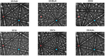
Eighteen different single-phase materials, comprising 6 of the 10 space groups within the  $\lpar {4/m\comma \;\bar{3}\comma \;\;2/m} \rpar$ point group, were selected for demonstrating the proposed space group classification methodology. Suitable samples for the remaining four space groups could not be obtained. This point group was chosen as it contains space groups that are very similar structurally and represent a significant classification challenge for conventional EBSD. The method of fabrication and homogenization (if applicable) for each sample is listed in Supplementary Table A1. The homogenization heat treatments were performed for three weeks in an inert atmosphere at temperatures guided by each phase diagram. Samples were mounted, polished to 0.05 μm colloidal silica, and then vibratory polished with 0.05 μm alumina for several hours.
Electron Backscatter Diffraction Pattern Collection
EBSD patterns (EBSPs) were collected in a Thermo-Fisher (formerly FEI) Apreo scanning electron microscope (SEM) equipped with an Oxford Symmetry EBSD detector. The Oxford Symmetry EBSD detector was utilized in high resolution (1244 × 1024) mode. The geometry of the set-up was held constant for each experiment. The working distance was 18.1 mm ± 0.1 mm. Aztec was used to set the detector insertion distance to 160.2 and the detector tilt to −3.1. The imaging parameters were 20 kV accelerating voltage, 51 nA beam current, 0.8 ms ± 0.1 ms dwell time, and 30 pattern averaging.
After collecting high-resolution EBSPs from each material, all patterns collected were exported as tiff images. Supplementary Figure A1 in the Appendix shows example images of the high-resolution diffraction patterns collected from the materials utilized in this study, organized by space group. All collected data for each material were individually assessed by the neural network, and the collection of images for each sample may contain partial or low-quality diffraction patterns, which will decrease the accuracy of their identification. See Supplementary Figure A2 for the inverse pole figures (IPFs) for each material. The IPFs were constructed using the MTEX software package (Bachmann et al., Reference Bachmann, Hielscher and Schaeben2010). The data in Supplementary Figure A2 were first plotted using the scale bars set automatically by MTEX to show the fine distribution of the data, and then with the scale bar fixed from 0 to 5 times random for the purpose of demonstrating the data does not approach medium texture levels. Analysis shows the experimental datasets have very low texture, typically in the range of two to three multiples of uniform distribution (M.U.D.) also referred to as times random. Typically, 5–10 is considered medium texture and greater than 10 is considered strong texture.
See Supplementary Figure A3 for histograms of mean angular deviation (MAD) and band contrast (BC) to compare pattern quality for each material. Each plot is also annotated with the mean (μ) and standard deviation (σ). The purpose of not filtering the test data was to assess the model as it would be applied in practice. Only the training sets were visually inspected to confirm high-quality diffraction patterns (no partial patterns) were utilized in fitting the neural network.
Neural Network Architecture
The well-studied convolutional neural network architecture Xception (Chollet, Reference Chollet2017) was selected as the basis architecture for fitting a model that determines which space group a diffraction pattern originated from. Supplementary Figure A4 in the appendix details a schematic of the convolutional neural network operating on an EBSP. For a complete description of the Xception architecture, please refer to Figure 5 in (Chollet, 2017).
Neural Network Training
Training was performed using 400 diffraction patterns per space group, evenly divided between the number of materials the model had access to during training. For example, if the model was given two materials during training, 200 diffraction patterns per material were made available. The validation set contained 100 diffraction patterns per space group, equivalent to the standard 80:20 train/validation split. The test set contains the rest of the patterns that were not used for training or validation. Model hyperparameters were selected or tuned as follows. Adam optimization with a learning rate of 0.001 (Kingma & Ba, Reference Kingma and Ba2014), and a minimum delta of 0.001 as the validation loss were employed for stopping criteria. The weight decay was set to 1e−5 following previous optimization work (Chollet, Reference Chollet2017). The CNNs were implemented with TensorFlow (Abadi et al., Reference Abadi, Barham, Chen, Chen, Davis, Dean, Devin, Ghemawat, Irving, Isard, Kudlur, Levenberg, Monga, Moore, Murray, Steiner, Tucker, Vasudevan, Warden, Wicke, Yu, Zheng and Brain2016) and Keras (Chollet, Reference Chollet2015). The code for implementing these models can be found at https://github.com/krkaufma/Electron-Diffraction-CNN or Zenodo (DOI: 10.5281/zenodo.3564937).
Diffraction Pattern Classification
Each diffraction pattern collected, but not used in training (>140,000 images), was evaluated in a random order by the corresponding trained CNN model without further information. The output classification of each diffraction pattern was recorded and saved in a (.csv) file and are tabulated in the Appendix. All corresponding bar plots of these data were generated with MATLAB. Precision and recall were calculated for each material and each space group using Scikit-learn (Pedregosa et al., Reference Pedregosa, Varoquaux, Gramfort, Michel, Thirion, Grisel, Blondel, Prettenhofer, Weiss, Dubourg, Vanderplas, Passos, Cournapeau, Brucher, Perrot and Duchesnay2011). Precision (equation 1) for each class (e.g., 225) is defined as the number of correctly predicted images out of all patterns predicted to belong to that class (e.g., 225). Recall is the number of correctly predicted patterns for each class divided by the actual number of patterns for the class (equation 2).
 $${\rm Precision} = \displaystyle{{{\rm true\;positives}} \over {{\rm true\;positives} + {\rm false\;positives}}}$$
 $${\rm Recall} = \displaystyle{{{\rm true\;positives}} \over {{\rm true\;positives} + {\rm false\;negatives}}}$$
Neural Network Interpretability
Gradient-weighted class activation mapping (Grad-CAM) was employed to provide insight into the deep neural network (Selvaraju et al., Reference Selvaraju, Cogswell, Das, Vedantam, Parikh and Batra2017). This method computes the importance of local regions in the diffraction image, normalizes them from 0 to 1, and is overlaid as a localization heatmap highlighting the important regions in the image. The “guided” backpropagation modifier was used to achieve pixel-space gradient visualizations and filter out information that suppresses the neurons. This information can be safely filtered out since we are only interested in what image features the neuron detects with respect to the target space group. The gradients flowing into the final convolution layer were targeted for two reasons: (i) convolutional layers naturally retain spatial information unlike the fully-connected layers and (ii) previous works have asserted that with increasing depth of a CNN, higher-level visual constructs are captured (Bengio et al., Reference Bengio, Courville and Vincent2013; Mahendran & Vedaldi, Reference Mahendran and Vedaldi2016).
Results and Discussion
The model is first trained on one material from each of six space groups in the  $\lpar {4/m\comma \;\bar{3}\comma \;\;2/m} \rpar$ point group; there are 10 space groups within the ( $4/m\comma \;\bar{3}\comma \;\;2/m\rpar$ point group, but suitable samples for 4 of these space groups could not be obtained. The first iteration uses the material with the largest formula weighted atomic number $\lpar \bar{Z}\rpar$ (i.e., atomic scattering factor) in order to establish a baseline performance. Ta was used as the training material for space group 229 instead of W since training would require nearly 50% of the available W diffraction patterns. Since W and Ta only differ by one atomic number, Ta will serve as a good baseline measurement and provide information about small steps in
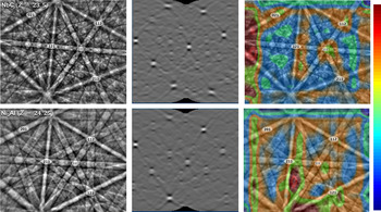
  $\bar{Z}$. This baseline will be compared to models trained using materials with a reduced number of visible reflectors resulting from lower atomic scattering factors. Figure 1 demonstrates this effect using a similarly oriented experimental diffraction pattern from Al and Ni with the same four zone axes labeled. The diffraction pattern from Ni has significantly more observable information (Kikuchi bands) since the atomic scattering factor is modulating their intensity. Using a limited number of materials (e.g., one) to represent the entire population of the space group when the neural network is learning the filters that maximize classification accuracy is likely to yield representations that are not as effective when Kikuchi bands are more or less visible based on diffraction intensity.

Fig. 1. Effect of atomic scattering factors on observable Kikuchi bands. Al (Z = 13) and Ni (Z = 28). Despite belonging to the same space group, the symmetry information visible for the lower atomic number Al is noticeably reduced compared with Ni.
Figure 2 shows the normalized accuracy of the first iteration of the model at classifying each of the 18 materials to the correct space group after learning from one material per class. Using only one material during training creates a significant opportunity for the neural network to “invent” representations that are not based on space group symmetry. The number of patterns from a given material that were classified to each space group is given in Appendix Supplementary Table A1. As shown in Figure 2, the model performs significantly better than random guessing (the dashed line at 16.7%) on multiple materials, including 6 of the 12 materials that were not in the training set. Of those 6, it achieves better than 45% accuracy on 4 of them: (Ni3Al, Cr3Si, W, and Al4Ni3). This is a good indicator that the model is learning useful features for differentiating the space groups, instead of trivial ones that only work during the training process. Furthermore, analysis of the IPFs in Supplementary Figure A2 shows that these materials can have distinctly different orientation distributions. As an example, the Al4Ni3 sample has a greater distribution of data with orientations near [001] in X, Y, and Z than the material used in training (Al4CoNi2). Yet, the model achieves 95% accuracy on Al4Ni3. From Supplementary Table A1, the overall accuracy of the model is 51.2%, well above the 16.7% chance of guessing correctly. It is observed that new materials with similar atomic scattering factors to the training material tend to have higher classification accuracy. Mo3Si and Cr3Si demonstrate that large differences in atomic scattering factor is not the penultimate factor and does not prevent accurate classification when evaluating new materials. There are also several materials with similar average Z that are rarely misclassified as one another. These include NiAl  $\lpar {\bar{Z} = 20.5} \rpar$, FeAl $\lpar {\bar{Z} = 19.5} \rpar$, and Cr3Si $\lpar {\bar{Z} = 21.5} \rpar$ as well as Ni3Al $\lpar {\bar{Z} = 24.25} \rpar$ and NbC $\lpar {\bar{Z} = 23.5} \rpar$.

Fig. 2. Plots of normalized classification accuracy after fitting the model with the high atomic number materials. (a) Space group 221; trained on FeNi3. (b) Space group 223; trained on Mo3Si. (c) Space group 225; trained on TaC. (d) Space group 227; trained on Ge. (e) Space group 229; trained on Ta. (f) Space group 230; trained on Al4CoNi2. The dashed line represents the chance of randomly guessing the correct space group. The formula weighted atomic number is located below each material.
Studying the misclassification events in Supplementary Table A1 provides further valuable insight. For example, the FeAl and NiAl samples are both B2, an ordered derivative of the BCC lattice, and the highest number of misclassifications for these two materials belong to space group 229 and 230. Figure 3 shows the difficulty of distinguishing these two space groups, a common problem in the literature (Gao et al., Reference Gao, Yeh, Liaw and Zhang2016; Li et al., Reference Li, Gazquez, Borisevich, Mishra and Flores2018).

Fig. 3. Comparison of diffraction patterns from B2 FeAl (space group 221) and BCC Fe (space group 229). B2 FeAl and BCC Fe can produce nearly identical diffraction patterns despite belonging to two different space groups.
Using the previous model as a baseline, the next three iterations study the effect of swapping the material used to represent a space group with the lowest average atomic number material in the dataset. First, TaC was replaced with Al in space group 225. The results of the exchange is shown in Figure 4 and Supplementary Table A2 in the Appendix. The plots in Figure 4 look largely unchanged except for space group 225 (Fig. 4c), for which materials with the lowest atomic scattering factors are now the most accurately classified. Furthermore, Supplementary Table A2 shows that the incorrect classifications for all other space groups are now primarily space group 225.

Fig. 4. Plots of normalized classification accuracy after fitting the model with a single low atomic number material. (a) Space group 221; trained on FeNi3. (b) Space group 223; trained on Mo3Si. (c) Space group 225; trained on Al. (d) Space group 227; trained on Ge. (e) Space group 229; trained on Ta. (f) Space group 230; trained on Al4CoNi2. The dashed line represents the chance of randomly guessing the correct space group. The formula weighted atomic number is located below each material.
In order to confirm the effects observed by exchanging Al for TaC in space group 225 previously, Si is exchanged with Ge in space group 227 (Fig. 5 and Supplementary Table A3). The training set for space group 225 is returned to TaC. The two space groups most affected by this change are 225 and 227, which both have FCC symmetry elements. For both space groups, as well as Fe, the use of Si as the training material causes diffraction patterns to be primarily misclassified as space group 221. The substitution of Si does result in the beneficial effect of increasing the classification accuracy of materials belonging to space group 221.

Fig. 5. Plots of normalized classification accuracy after fitting the model with a single low atomic number material. (a) Space group 221; trained on FeNi3. (b) Space group 223; trained on Mo3Si. (c) Space group 225; trained on TaC. (d) Space group 227; trained on Si. (e) Space group 229; trained on Ta. (f) Space group 230; trained on Al4CoNi2. The dashed line represents the chance of randomly guessing the correct space group. The formula weighted atomic number is located below each material.
The last swap studied was the lower atomic number Fe in place of Ta (Fig. 6). Similar to what was observed when Al was used in space group 225, the increased correct classifications have shifted toward the low atomic number materials within space group 229. Furthermore, the B2 materials are now primarily misclassified as belonging to the BCC symmetry space group 229 (Supplementary Table A4). In comparison to Supplementary Table A1, almost half of the NiAl diffraction patterns were classified as 229 instead of 230. These three examples confirm that providing the neural network with only the lightest or heaviest materials will result in avoidable misclassification events.

Fig. 6. Plots of normalized classification accuracy after fitting the model with a single low atomic number material. (a) Space group 221; trained on FeNi3. (b) Space group 223; trained on Mo3Si. (c) Space group 225; trained on TaC. (d) Space group 227; trained on Ge. (e) Space group 229; trained on Fe. (f) Space group 230; trained on Al4CoNi2. The dashed line represents the chance of randomly guessing the correct space group. The formula weighted atomic number is located below each material.
Previously, the model has only been supplied with information from one material to learn from. It should not be surprising that the limited data representing the population of all materials in each class results in misclassification events when extrapolating further away from the training data. To demonstrate the increased accuracy of the technique when the data begins to better represent the population, we add a second material to the training set for space groups 221, 225, 227, and 229. Materials were not added to space group 223 and 230 since performance on those two groups was already well above the probability of the neural network guessing correctly by chance (16.7%) for the second material. The total number of diffraction patterns available to the neural network during training remained fixed as described in the Methods section. Supplementary Figures A5, A6 display the IPFs and histograms, respectively, for the training data used in this model. As evidenced by the low M.U.D. and wide range of pattern quality, the data provided to the model during training is quite diverse. The classification results with new diffraction patterns are shown in Figure 7 and Supplementary Table A5 in the Appendix. Compared to the neural networks trained with only one material, this model has 29% higher accuracy (now 80% correct) and demonstrates significantly improved accuracy on materials not utilized in the training set. For example, diffraction patterns from Ni3Al, FeAl, Cr3Si, NbC, TiC, and Al4CoNi2 are correctly classified significantly more than random guessing even though the neural network was not provided diffraction patterns from these materials from which to learn. Moreover, significantly increasing the range of atomic scattering factors, such as in Figures 7a, 7c, improves the neural network's performance on materials with scattering factors further outside the range. Aluminum and tungsten are the only two materials where the neural network's classification accuracy is below the probability of randomly guessing the correct answer. An analysis of the orientations and pattern quality for patterns that were correctly identified and misclassified was performed on several materials outside the training set. NbC, Al, and W were selected in order to make a number of comparisons including materials with varying classification accuracy or within the same space group. Supplementary Figure A7 shows that for each material, the IPFs for the correctly classified patterns resembles the IPFs for patterns that were misclassified. In other words, specific orientations do not seem to be more likely to be classified correctly. Supplementary Figure A8 shows the corresponding MAD and BC histograms. While the plots and associated statistics for NbC show patterns with lower band contrast or higher MAD have a slight tendency to be misclassified, there does not appear to be a strong relationship between these pattern quality metrics and classification accuracy.

Fig. 7. Plots of normalized classification accuracy after fitting the model. (a) Space group 221; trained on FeNi3 and NiAl. (b) Space group 223; trained on Mo3Si. (c) Space group 225; trained on TaC and Ni. (d) Space group 227; trained on Ge and Si. (e) Space group 229; trained on Ta and Fe. (f) Space group 230; trained on Al4CoNi2. The dashed line represents the chance of randomly guessing the correct space group. The formula weighted atomic number is located below each material.
The excellent overall performance of the neural network in correctly identifying the space group necessitates an understandable interpretation of what information is important to the model, since orientation and pattern quality are not seemingly biasing the results of this study. Figure 8 is a set of “visual explanations” for the decisions made by the Hough-based method and the trained CNN from Figure 7. The selected diffraction patterns (Fig. 8 left-side) from NbC and Ni3Al are of nearly the same orientation and average atomic number but are from space group 225 and 221, respectively. Importantly, the model had not trained on any EBSPs from these two materials at this point. The Hough-based method produces the “butterfly peak” (Christian et al., Reference Lassen1994) representation (Fig. 8 middle) for matching the interplanar angles to user selected libraries. The resulting Hough-transforms are nearly identical for both NbC and Ni3Al, save for minor differences owing to the small orientation shift. Furthermore, the Hough-based method creates a sparse representation that does not capture the finer detail found within the EBSPs. For example, the [111] and [112] zone axes are each encircled by a discernable HOLZ ring (Michael & Eades, Reference Michael and Eades2000) as well as excess and deficiency features (Winkelmann, Reference Winkelmann2008). In comparison to the Hough method, the convolutional neural network can learn these features, or lack of them, and associate them with the correct space group. Using gradient-weighted class activation mapping (Grad-CAM) (Selvaraju et al., Reference Selvaraju, Cogswell, Das, Vedantam, Parikh and Batra2017), we produce a localization heatmap highlighting the important regions for predicting the target class (Fig. 8 right-side). When visually inspecting the importance of local regions to the neural network, it is immediately observed that the neural network finds each of the labeled zone axes to be of high importance (orange in color) in both EBSPs. In fact, the heatmaps look remarkably similar and are concentrated about the same features a crystallographer would use. These features clearly include the zone axes and HOLZ rings. To investigate this further, a diffraction pattern is simulated for each material using EMSoft (Callahan & De Graef, Reference Callahan and De Graef2013). In Figure 9, it is first observed that many of the features of the patterns are similar, such as Kikuchi bands and diffraction maxima. These similarities explain why the Hough transform-based method cannot distinguish the two. However, it is also immediately noticeable that equivalent zone axes and surrounding regions have very different appearances. As examples, two sets of equivalent zone axes have been marked with either a red triangle or blue hexagon. The red triangle is the equivalent to the [111] zone axis studied in Figure 8. While the fidelity of the simulated patterns with experimental patterns is not perfect, the existence of the discussed features can be confirmed by comparing them with the experimental patterns previously discussed. For example, compare the red and blue labeled zone axes in Figure 9 for Ni and Mo3Si with the experimental NbC (Fig. 8) and Cr3Si (Supplementary Fig. A1) diffraction patterns. The structure and features visible are clearly well correlated.

Fig. 8. Comparison of feature detection with Hough-based EBSD and the trained CNN. (Top row from left to right) Experimental EBSP from NbC (space group 225; FCC structure), Hough-based feature detection, and gradient-weighted class activated map. (Bottom row from left to right) Experimental EBSP from Ni3Al (space group 221; L12 structure), Hough-based feature detection, and gradient-weighted class activated map. The importance scale for the heatmaps goes from dark blue (low) to dark red (high).

Fig. 9. Dynamically simulated EBSPs. One diffraction pattern per space group was simulated to study the expected differences and assess the feature importance observed in experimental patterns. The observed reflectors are similar for each space group; however, attributes nearby the zone axes can vary significantly. Two sets of equivalent zone axes have been indicated with either a red triangle or blue hexagon.
Supplementary Figure A9 helps to elucidate the failure mechanism of this model by studying the activations of the current model, which incorrectly identified the pattern, compared to the activations in the first model, which had correctly identified the same EBSP. In each case, the heatmaps for space group 229 are overlaid onto the diffraction pattern. When correctly identified as belonging to space group 229 (Supplementary Fig. A9, center), significantly more zone axes are given higher importance scores than when misclassified to space group 225 (Supplementary Fig. A9, right). The same is observed with features within the HOLZ rings, such as near the [001] and [101] axis. It is important to note, the similarity between the activations at zone axes, such as [001], [012], and [102], should not be surprising since the activations for class 229 are being studied. Failures such as this can potentially be alleviated as the number of samples, experimental or simulated, used in fitting these models continues to grow. Previous works using experimental (Kaufmann et al., Reference Kaufmann, Zhu, Rosengarten, Maryanovsky, Harrington, Marin and Vecchio2020) and simulated (Foden et al., Reference Foden, Previero and Britton2019) patterns have further demonstrated the attentiveness of the last layers of the model on the zone axes and surrounding features. The study using simulated patterns also elucidated each convolutional layer's attention to specific aspects of EBSPs including edges and major Kikuchi bands. These studies into the “visual” perception of the model suggest that the network has learned relevant and intuitive features for identifying space groups.
By providing the neural network with diffraction patterns from many materials, the neural network can improve its resiliency to small changes within a space group, simultaneously developing a better understanding of what elements in the image are most useful and learning filters that better capture the information. Figure 10 demonstrates this by supplying the same number of diffraction patterns to learn from as used previously, but evenly divided between all available materials in each space group. Supplementary Table A6 shows the number of images classified to each space group from individual materials. The classification accuracy has increased to 93%, compared to 40–65% for the models that were only provided with one training material per space group (Figs. 2, 4–7) and 80% when using two materials for some of the classes (Fig. 8).

Fig. 10. Plots of normalized classification accuracy after fitting the model with data from each material. (a) Space group 221. (b) Space group 223. (c) Space group 225. (d) Space group 227. (e) Space group 229. (f) Space group 230. The dashed line represents the chance of randomly guessing the correct space group. The formula weighted atomic number is located below each material.
Conclusion
In this paper, a high-throughput CNN-based approach to classifying electron backscatter diffraction patterns at the space group level is developed and demonstrated. In each study, the CNN is shown to be able to classify at least several materials outside the training set with much better probability than random guessing. Several investigations are conducted to explore the potential for biases owing to crystallographic orientation, pattern quality, or physical phenomena. The number of visible reflectors, directly correlated with atomic scattering factors, is found to have an impact classification accuracy when only low or high atomic number materials are used to fit the model. Increasing the range of atomic scattering factors used in training each class is found to reduce the number of misclassification events caused by large differences in the number of visible reflectors. The dataset for each material and space group were of very low texture and good distributions of pattern quality metrics. Continued inclusion of data, particularly from more materials, will likely increase the robustness of the model when presented with new data. Investigation of the convolutional neural network's inner workings, through visualization of feature importance, strongly indicates the network is using the same features a crystallographer would use to manually identify the structure, particularly the information within the HOLZ rings. This analysis, combined with IPFs, suggests there is minimal orientation bias present. We believe this method can be expanded to the remaining space groups and implemented as part of a multi-tiered model for determining the complete crystal structure. There are no algorithmic challenges to extending this framework to all 230 space groups, it is only currently limited by the lack of data, which simulated EBSD patterns may help to resolve. This technique should benefit from continued advancements in detectors, such as direct electron detectors, and the framework is expected to be immediately applicable to similar techniques such as electron channeling patterns and CBED. A wide range of other research areas including pharmacology, structural biology, and geology are expected to benefit by using similar automated algorithms to reduce the amount of time required for structural identification.
Supplementary material
To view supplementary material for this article, please visit https://doi.org/10.1017/S1431927620001506
Acknowledgments
The authors would like to thank Wenyou Jiang, William Mellor, and Xiao Liu for their assistance. K. Kaufmann was supported by the Department of Defense (DoD) through the National Defense Science and Engineering Graduate Fellowship (NDSEG) Program. K. Kaufmann would also like to acknowledge the support of the ARCS Foundation, San Diego Chapter. KV would like to acknowledge the financial generosity of the Oerlikon Group in support of his research group.


 Open access