


Introduction
Electron probe microanalysis (EPMA) is an analytical technique widely used for the determination of the chemical composition of materials (Llovet et al., Reference Llovet, Moy, Pinard and Fournelle2021). The incorporation of multilayer pseudocrystals and grating monochromators in electron beam instruments has stimulated the use of soft X-rays (<1 keV), which have certain advantages over the conventional higher energy X-rays (Pouchou, Reference Pouchou1996). However, soft X-rays generally involve valence electrons, which are affected by chemical bonding. Because matrix corrections do not include corrections for chemical bonding, the use of soft X-rays for chemical analysis often results in large errors in the evaluated concentrations (Pouchou, Reference Pouchou1996; Llovet et al., Reference Llovet, Heikinheimo, Núñez Galindo, Merlet, Almagro Bello, Richter, Fournelle and van Hoek2012; Gopon et al., Reference Gopon, Fournelle, Sobol and Llovet2013; Llovet et al., Reference Llovet, Pinard, Heikinheimo, Louhenkilpi and Richter2016). To overcome these difficulties, alternative strategies have been developed (e.g., Gopon et al., Reference Gopon, Fournelle, Sobol and Llovet2013; Buse & Kearns, Reference Buse and Kearns2018; Moy et al., Reference Moy, Fournelle and von der Handt2019a, Reference Moy, Fournelle and von der Handt2019b).
The situation is further complicated in certain cases because of the effect of self-absorption. This effect, also referred to as differential or preferential self-absorption (Armstrong, Reference Armstrong1999), occurs when an X-ray line is located near a broad absorption edge of the same element such that the high-energy side of the line straddles the rising edge (Fig. 1). As a result, a distortion to the X-ray line shape is produced, which depends on the excitation conditions (Liefeld, Reference Liefeld and Fabian1968; Chopra, Reference Chopra1970). This is the case, for example, of the L $\alpha$ and L $\beta$ X-ray lines of first-row transition metals, which correspond to the electron transition M $_{4, 5}$ $\rightarrow$ L $_3$ (3 $d_{5/2, 3/2}$ $\rightarrow$ 2 $p_{3/2}$) and M $_4$
$_4$  $\rightarrow$ L $_2$ (3 $d_{3/2}$ $\rightarrow$ 2 $p_{1/2}$), respectively. It is worth pointing out that although these transitions do not involve the outermost shells of these elements, the $3d$ shells are admixed to some extent with the valence band and therefore they are involved in the chemical bonding. Matrix corrections do not account for self-absorption effects as they implicitly assume that X-ray lines are narrow (and thus they neglect the variation of mass absorption coefficients over the width of X-ray lines).

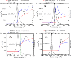
Fig. 1. Theoretical (PHOTACS) and experimental mass absorption coefficients of metallic Fe (a), Ni (b), Cu (c), and Zn (d) around the L $_3$ edge. See text for details. The corresponding emission L $\alpha$ lines, modeled as pure Lorentzian distributions with the indicated FWHM (see Table 2) are also shown (in arbitrary scale). For Fe and Ni, the high-energy side of the X-ray line straddles the rising edge, causing the effect of self-absorption. Conversely, for Cu and Zn, there is almost no overlap between the emission line and the absorption edge, and therefore, these elements are free from self-absorption effects. The black dashed and the green dashed vertical lines represent the location of the L $\alpha$ lines and L $_3$ edges, respectively (Deslattes et al., Reference Deslattes, Kessler, Indelicato, de Billy, Lindroth and Anton2003).
The effect of self-absorption in soft X-ray spectrometry by electrons has been known for decades (Fabian et al., Reference Fabian, Watson and Marshall1972). Soft X-ray spectroscopy provides valuable information about the electronic structure of solids and it was early recognized that self-absorption should be taken into account for a correct interpretation of measured spectra (Hanson & Herrera, Reference Hanson and Herrera1957; Liefeld, Reference Liefeld and Fabian1968). Hence, different correction procedures were developed (Crisp, Reference Crisp1977, Reference Crisp1980, Reference Crisp1983). Taking advantage of this effect, the so-called self-absorption (difference) spectroscopy was developed as an alternative to conventional X-ray absorption spectroscopy (Ulmer, Reference Ulmer1978, Reference Ulmer1981; Burgäzy et al., Reference Burgäzy, Jaeger, Schulze, Lamparter and Steeb1989). It is worth bearing in mind that the effect of self-absorption is common in spectroscopy (Cowan & Dieke, Reference Cowan and Dieke1948) and it may have a different meaning depending on the particular method. For instance, in conventional X-ray absorption spectroscopy, self-absorption refers to the distortion of the spectrum originated by the change in penetration depth of the incident photon beam as its energy is scanned across the absorption edge (Tröger et al., Reference Tröger, Arvanitis, Baberschke, Michaelis, Grimm and Zschech1992).
In the field of EPMA, the effect of self-absorption has been mainly exploited as the basis of methods to determine the Fe oxidation state. Fialin et al. (Reference Fialin, Wagner, Métric, Humler, Galoisy and Bézos2001) used the Fe L $\alpha$ peak shift due to self-absorption to obtain the Fe oxidation state in some minerals and glasses. Höfer & Brey (Reference Höfer and Brey2007) developed the so-called flank method, which essentially consists of measuring the L $\beta$/L $\alpha$ intensity ratio at energy positions suitably selected on a self-absorption spectrum, to obtain the Fe oxidation state in selected minerals. The effect of self-absorption has also been considered with a view to improving the spectral fitting of wavelength-dispersive spectra (Rémond et al., Reference Rémond, Campbell, Packwood and Fialin1993, Reference Rémond, Gilles, Fialin, Rouer, Marinenko, Myklebust and Newbury1996, Reference Rémond, Gilles, Fialin, Rouer, Marinenko, Myklebust and Newbury2002; Sepúlveda et al., Reference Sepúlveda, Rodríguez, Pérez, Bertol, Carreras, Trincavelli, Vasconcellos, Hinrichs and Castellano2017). However, the influence of self-absorption on quantitative analysis has been rarely addressed. This can be explained at least in part by the fact that errors due to neglecting self-absorption are difficult to disentangle from those arising from the large uncertainties in the mass absorption coefficients near absorption edges. Also, it should be noted here that for soft X-rays, the fluorescence yields may not cancel when taking the ratio of X-ray intensities because bonding differences between specimen and standard may result in a different fluorescence yield for each, resulting in an additional source of error (Nagel, Reference Nagel1969; Llovet et al., Reference Llovet, Pinard, Heikinheimo, Louhenkilpi and Richter2016).
In this study, we assess the error due to neglecting self-absorption in the analysis of first-row transition elements using L $\alpha$ lines. We focus on metallic Fe, Ni, Cu, and Zn, for which high-accuracy, experimental mass absorption coefficients have become recently available (Sokaras et al., Reference Sokaras, Kochur, Müller, Kolbe, Beckhoff, Mantler, Zarkadas, Andrianis, Lagoyannis and Karydas2011; Ménesguen et al., Reference Ménesguen, Gerlach, Pollakowski, Unterumsberger, Haschke, Beckhoff and Lépy2016, Reference Ménesguen, Lépy, Hönicke, Müller, Unterumsberger, Beckhoff, Hoszowska, Dousse, Blachucki, Ito, Yamashita and Fukushima2018). L $\alpha$ X-ray line shapes and intensities are calculated using an improved approach which takes into account both the Lorentzian shape of X-ray lines and the energy dependence of mass absorption coefficients near the absorption edge. By comparing the results of our calculations with those obtained assuming narrow X-ray lines and definite mass absorption coefficients, we are able to establish the errors arising solely from self-absorption.
Material and Methods
Self-absorption Calculations
Consider a specimen bombarded by a beam of electrons of energy  $E_{\rm 0}$ that impinge normally on the specimen surface. If we assume that X-ray lines are mono-energetic ( $\delta$-functions), the intensity $I_0$ of characteristic X-rays of energy $E_{\rm x}$ per incident electron per unit solid angle emitted by an element with concentration $c$ and collected at a take-off angle $\chi$ can be written as (Llovet et al., Reference Llovet, Moy, Pinard and Fournelle2021):
 $$I_0 = \epsilon ( E_{\rm x}) {N_{\rm A}\over A} c \omega p ( 1 + T_{\rm CK}) \sigma( E_{\rm 0}) ( 1 + {{\cal F}}) \int_0^{\infty} \Phi( \rho z) \exp -\left[{\mu\over \rho} ( E_{\rm x}) {\rho z\over \sin\chi} \right]{\rm d} \rho z,\; $$
where  $N_{\rm A}$ is Avogadro's number, $A$ is the atomic weight of the element, $\epsilon ( E_{\rm x})$ is the spectrometer efficiency evaluated at $E_{\rm x}$, $\omega$ is the fluorescence yield, $p$ is the line fraction, $\sigma ( E_{\rm 0})$ is the ionization cross section of the shell giving rise to the considered X-rays, $\Phi ( \rho z)$ is the depth distribution of ionization where $\rho$ is the mass density of the material and $z$ is the depth, $( \mu /\rho ) ( E_{\rm x})$ is the mean mass absorption coefficient evaluated at $E_{\rm x}$. The factor $( 1 + T_{\rm CK})$ is the Coster–Kronig factor, which takes into account the contribution from vacancies generated from an initial vacancy in another subshell of the same shell (for the sake of simplicity, the contribution from vacancies generated from an initial vacancy in another shell are disregarded) and $( 1 + {{\cal F}})$ is the fluorescence factor, which accounts for the enhancement due to X-ray fluorescence by primary X-rays and bremsstrahlung. Following the pioneering work of Castaing, $\Phi ( \rho z)$ is defined conventionally such that the number of ionizations for a given element and shell produced per electron at a depth between $\rho z$ and $\rho z + {{\rm d}} ( \rho z)$ is given by $( N_{\rm A}/A) c \sigma ( E_{\rm 0}) \Phi ( \rho z) \, {{\rm d}} ( \rho z)$. The mean mass absorption coefficient is calculated as
 $${\mu\over \rho} ( E_{\rm x}) = \sum_i c_i \left({\mu\over \rho}\right)_i ( E_{\rm x}) ,\; $$
where  $( \mu /\rho ) _i ( E_{\rm x})$ is the mass absorption coefficient of the $i$ absorber element with a mass fraction of $c_i$, evaluated at $E_{\rm x}$.
Direct determination of  $c$ from $I_{\rm x}$ using equation (1) is generally avoided because of the large uncertainties in parameters, such as $\epsilon$, $\omega$, or $\sigma$. To overcome this difficulty, the X-ray intensity emitted from the specimen is normalized to that emitted from a reference standard that contains the element of interest, which is measured under the same instrumental conditions. By doing so, the parameters outside the integral are assumed to cancel out, with the exception of the unknown concentration. The ratio of X-ray intensities is referred to as $k$-ratio ( $k$) and is written as:
 $$k = {I\over I^{\rm std}} = {c\over c^{\rm std}}\left\{{\displaystyle\int_0^{\infty} \Phi( \rho z) \exp \left[-\frac{\mu}{\rho} ( E_{\rm x}) \frac{\rho z}{\sin\chi} \right]{{\rm d}} \rho z \over \displaystyle\int_0^{\infty} \Phi^{\rm std}( \rho z) \exp \left[-\frac{\mu}{\rho}^{\rm std} ( E_{\rm x}) \frac{\rho z}{\sin\chi} \right]{{\rm d}} \rho z } \times {( 1 + {{\cal F}}) \over ( 1 + {{\cal F}}) ^{\rm std}}\right\},\; $$
where the superscript  ${\rm std}$ means that the corresponding quantity is evaluated in the reference standard. Equation (3) is the basis of quantitative analysis and, for each element making up the specimen, is solved for $c$ by using iterative methods. The factor inside the curly brackets is known as the matrix correction factor and takes into account the differences in electron transport and X-ray generation between specimen and standard, as well as X-ray absorption and fluorescence differential effects. Different parameterizations are available to calculate the $\Phi ( \rho z)$ function and $\mu /\rho$ values are available as numerical tables such as the FFAST tabulation (Chantler et al., Reference Chantler, Olsen, Dragoset, Chang, Kishore, Kotochigova and Zucker2005) or they can be calculated using empirical formulas (Heinrich, Reference Heinrich1986).
To take into account the effect of self-absorption, equation (1) needs to be suitably modified. For convenience, we will rewrite equation (1) as follows:
 $$I_0 = \epsilon( E_{\rm x}) I_{\rm g} {{\displaystyle\int_0^{\infty} \Phi( \rho z) \exp \left[- \frac{\mu}{\rho}( E_{\rm x}) \frac{\rho z}{\sin \chi} \right]{{\rm d}} \rho z}\over {\displaystyle\int_0^{\infty} \Phi( \rho z) \, {{\rm d}} \rho z}},$$
where  $I_{\rm g}$ is the intensity of primary photons, i.e. the total number of X-rays generated in the specimen per unit solid angle per electron, including the contributions from Coster–Kronig transitions and fluorescence, which is given by:
 $$I_{\rm g} = {N_{\rm A}\over A} c \omega p ( 1 + T_{\rm CK}) ( 1 + {{\cal F}}) \sigma( E_{\rm 0}) \int_0^{\infty} \Phi( \rho z) \, {{\rm d}} ( \rho z) ,\; $$
 We will assume that the X-ray line has a Lorentzian distribution  $L( E)$ defined by
 $$L( E) = {1\over \pi} {\Gamma/2\over ( E-E_{\rm x}) ^{2} + \Gamma^{2}/4},\; $$
where  $\Gamma$ is the full-width half maximum (FWHM) and
 $$\int_{-\infty}^{\infty} L( E) \, {{\rm d}}E = 1.$$
This assumption is justified since the energy distribution of an X-ray line is the convolution of energy distributions of the two involved levels, which have Lorentzian shapes if they are atomic levels. Thus, the energy distribution of an X-ray line has a Lorentzian distribution with FWHM equal to the sum of the FWHM of the two participating levels. In the case of the L $\alpha$ and L $\beta$ lines of the first-row transition elements, although the $3d$ shells are admixed to some extend with the valence band, it has been shown that the lines can be satisfactorily described by Lorentzian distributions (Dev & Brinkman, Reference Dev and Brinkman1972). The energy distribution $I( E)$ of X-rays collected by the spectrometer per unit solid angle per electron can then be written as:
 $$I( E) = \epsilon( E) I_{\rm g} L( E) {{\displaystyle \int_0^{\infty} \Phi( \rho z) \exp \left[- \frac{\mu}{\rho}( E) \frac{\rho z}{\sin\chi} \right]{{\rm d}} \rho z}\over {\displaystyle\int_0^{\infty} \Phi( \rho z) \, {{\rm d}} \rho z}} ,\; $$
where ( $\mu /\rho ) ( E$) is the energy-dependent absorption coefficient. Equation (8) has to be numerically integrated to obtain the X-ray line distribution.
The intensity of the X-ray line is given by the area under  $I( E)$. Note that because the Lorentzian distribution extends to infinity, a relative large integration interval needs to be selected for the integral of $I( E)$ to be accurate. If we set ( $\mu /\rho ) ( E) = ( \mu /\rho ) ( E_{\rm x}$) in equation (8), and we assume that $\epsilon ( E)$ does not change significantly over the integration interval, the area under $I( E)$ is equal to the intensity $I_0$ obtained from equation (4). The usual practice in EPMA is to measure the X-ray intensity at the peak height $I_{\rm h}$ instead of the peak area, i.e. $I_{\rm h} = \max { I( E) }$. This implicitly assumes that the peak height is proportional to the peak area. Because of this, we can assess the error made in disregarding the energy dependence of the mass absorption coefficient, which gives rise to self-absorption, by comparing the maximum of $I( E)$ [equation (8)] with the maximum of $I_0( E)$ obtained as
 $$I_0( E) = \epsilon( E) I_{\rm g} L( E) {{\displaystyle\int_0^{\infty} \Phi( \rho z) \exp \left[- \frac{\mu}{\rho}( E_{\rm x}) \frac{\rho z}{\sin\chi} \right]{{\rm d}} \rho z}\over {\displaystyle\int_0^{\infty} \Phi( \rho z) \, {{\rm d}} \rho z}},\; $$
i.e. by replacing ( $\mu /\rho ) ( E$) by ( $\mu /\rho ) ( E_{\rm x}$) in equation (8).
Monte Carlo Simulations
The X-ray intensities per unit solid angle per electron generated in the specimens,  $I_{\rm g}$, and the $\Phi ( z)$ distributions were calculated using the Monte Carlo simulation program PENEPMA (Llovet & Salvat, Reference Llovet and Salvat2017). This program performs Monte Carlo simulation of EPMA measurements and provides the intensities of X-rays emitted at a specific direction, split into the different components (primary X-rays, characteristic fluorescence, and continuum fluorescence). PENEPMA also provides other quantities of interest, such as $I_{\rm g}$ and $\Phi ( z)$.Footnote 1 Note that to obtain $\Phi ( z)$, the user must specify the coordinates of the vertices of a box where the space distribution of X-ray emission will be scored for the selected X-ray line or X-ray energy interval. Here, we point out that the X-ray depth distribution given by PENEPMA has dimensions of cm $^{-1}$ and it is normalized to the total number of emitted X-rays per incident electron, while the depth distribution used in conventional EPMA is dimensionless and its integral does not correspond to the total number of emitted X-rays (see above).
In PENEPMA, electron trajectories are simulated by using an algorithm which combines detailed simulation of interactions with large angular deflections and the energy losses with a “condensed” simulation of interactions with small deflections and energy losses. The simulation algorithm is specified by means of several parameters and it can be further optimized by forcing selected interactions using variance reduction techniques. Accordingly, in addition to the parameters that characterize their experiment (e.g., electron beam energy, sample composition and geometry, detector aperture, and take-off angle), the user must specify the simulation and forcing parameters. A summary of the simulation and forcing parameters used in this work is given in Table 1 (for a detailed explanation, see Salvat, Reference Salvat2019).
Table 1. Summary of the Simulation Parameters Used in the PENEPMA Simulations.

Experimental Method
X-ray emission spectra around the positions of the Ni L $\alpha$ and L $\beta$ peaks were measured on a metallic Ni target using a JEOL JXA-8230 electron microprobe operated in wavelength-dispersive mode. Spectra were acquired at 2, 10, 15, and 30 kV accelerating voltage using a 140-mm radius Johann-type spectrometer with a thallium acid phthalate (TAP) crystal ( $2d = 2.5757$ nm) and a spectrum channel width of 2 $\mu$m. A 300- $\mu$m diameter collimator slit (the smallest available) was used to minimize X-ray beam divergence and defocusing arising from the Johann focusing geometry, thus ensuring the highest possible spectral resolution.
To minimize the uncertainties arising from counting statistics, lengthy counting times (4 h each spectrum) and high-beam currents (400 nA) were used for the measurements. The number of channels was 7500 and the dwell time was 2 s. Furthermore, to minimize carbon contamination during measurements, the sample was cleaned for 10 min in the microprobe exchange chamber using a plasma cleaner (Evactron 25, Xei Scientific) and a defocused beam with a 10  $\mu$m spot was used during the acquisitions. The spectra were smoothed using the automatic option of the microprobe software. The reproducibility of the wavescans was assessed by repeated acquisitions of the Ni L $\alpha$ spectra at 20 kV accelerating voltage. It was found that the peak position could be reproduced to within $\pm$0.1 eV.
Results and Discussion
Self-absorption of Diagram Lines
As discussed earlier, the natural width of an X-ray line can be obtained from the widths of the two participating levels. Atomic-level widths for atomic levels K to N $_7$ were compiled by Campbell & Papp (Reference Campbell and Papp2001) from available experimental data but, unfortunately, they do not include data for the M $_{4, 5}$ levels of Ni, Cu, Fe, and Zn, which are needed to calculate the L $\alpha$ line widths. Experimental natural L $\alpha$ line widths for metallic Fe, Ni, Cu, and Zn have been reported by Bonnelle (Reference Bonnelle1966), Faessler (Reference Faessler2013), Rémond et al. (Reference Rémond, Myklebust, Fialin, Nockfolds, Phillips and Roques-Carmes2002), and Sepúlveda et al. (Reference Sepúlveda, Rodríguez, Pérez, Bertol, Carreras, Trincavelli, Vasconcellos, Hinrichs and Castellano2017), which are listed in Table 2. In this work, we have arbitrarily adopted the natural FWHMs reported by Bonnelle for Fe (3.7 eV) and Ni (2.58 eV) and by Faesler for Cu (3.7 eV), and Zn (1.7 eV).
Table 2. Experimental Line Widths for L $\alpha$ Lines.

Figure 1 shows the Fe, Ni, Cu, and Zn L $\alpha$ emission lines, modeled as Lorentzian distributions, together with the experimental mass absorption coefficients reported by Sokaras et al. (Reference Sokaras, Kochur, Müller, Kolbe, Beckhoff, Mantler, Zarkadas, Andrianis, Lagoyannis and Karydas2011) for Fe, Ménesguen et al. (Reference Ménesguen, Lépy, Hönicke, Müller, Unterumsberger, Beckhoff, Hoszowska, Dousse, Blachucki, Ito, Yamashita and Fukushima2018) for Ni, and Ménesguen et al. (Reference Ménesguen, Gerlach, Pollakowski, Unterumsberger, Haschke, Beckhoff and Lépy2016) for Cu and Zn. For the sake of simplicity, we have assumed that $\epsilon ( E)$ is constant over the extension of the X-ray line. For Fe and Ni, both the L $\alpha$ line and the L $_3$ absorption edge are relatively broad and the edge extends in part over the line. Because $( \mu /\rho ) ( E)$ increases rapidly across the X-ray line, the high-energy side of the line is expected to be more attenuated than the low-energy side, leading to a distortion to the line shape.
In the case of Ni, the absorption spectrum shows a white line at the L $_3$ edge.Footnote 2 For most elements in metallic states, white lines arise when there are electronic states with a high density of unoccupied states (Wei & Lytle, Reference Wei and Lytle1979). For Ni, as well as for most of the first-row transition metals, white lines originate from transitions between the $2p$ level and the unoccupied $3d$ states. The white line appears to be less intense for Fe. Here we note that other photoabsorption cross section measurements available in the literature show a more intense white line at the Fe L $_3$ edge (del Grande, Reference del Grande1990; Lee et al., Reference Lee, Xiang, Ravel, Kortright and Flanagan2009). Yet, we prefer to use Sokaras et al.'s data here mainly because their mass absorption coefficient value at $E_{\rm x} = 704.8$ eV (the Fe L $\alpha$ line energy) is 3510 cm $^{2}$/g, which is in much better agreement with the measured values of 3350 cm $^{2}$/g (Pouchou & Pichoir, Reference Pouchou and Pichoir1988) and of 3639 cm $^{2}$/g (Gopon et al., Reference Gopon, Fournelle, Sobol and Llovet2013), than the value of 5151 cm $^{2}$/g obtained from Lee et al.'s data (we also note here that it was not possible to accurately extract numerical data from del Grande's article).
In contrast with Fe and Ni, the absorption spectra of Cu and Zn show step-like profiles, with some oscillations above the edges. These oscillations are generally referred to as extended X-ray absorption fine structure (EXAFS). The overlap of the L $\alpha$ line with the L $_3$ absorption edge is very small for Cu and there is no overlap for Zn. In the latter case, the mass absorption coefficient is almost constant across the emission line, thus no distortion to the X-ray shape line is expected.
Figure 1 also displays the theoretical mass absorption coefficients calculated using the program PHOTACS of Sabbatucci & Salvat (Reference Sabbatucci and Salvat2016). Photoelectric cross sections obtained with this program have been recently implemented in the PENELOPE subroutine package (Salvat, Reference Salvat2019) used by PENEPMA. In our calculations, the effect of finite mean life of the excited states (natural level width) was included, which causes the edges to follow an arctangent curve instead of an ideal sharp saw-tooth shape (see e.g., Ritchtmyer et al., Reference Ritchtmyer, Barnes and Ramberg1934). Note that calculations using PHOTACS apply to free atoms (gases) and consequently they do not include those features arising from solid-state effects such as the white lines [PHOTACS can include the contribution from excited (atomic) states, which would be visible in measurements in gases]. This may explain in part why a good agreement is observed between the calculated and the experimental L $_3$ edge positions for Cu and Zn, owing to the fact that the spectra of these metals do not show white lines.
In Figure 2, the Fe, Ni, Cu, and Zn L $\alpha$ line shapes for 30 keV electron excitation calculated using equation (8) (with the energy-dependent mass absorption coefficients shown in Fig. 1) are compared with those obtained using equation (9). For the latter calculations, we use the $\mu /\rho$ values extracted from the above-mentioned energy-dependent mass absorption coefficients at the corresponding line energies, which are summarized in Table 3.

Fig. 2. L $\alpha$ X-ray emission lines for Fe (a), Ni (b), Cu (c), and Zn (d) for 30 keV electron excitation calculated using equation (8) and the energy-dependent mass absorption coefficients shown in Figure 1 and using equation (9) with the definite mass absorption coefficients tabulated in Table 3. Using equation (8), we simulate an actual measurement, while by using equation (9), we simulate the calculations performed by matrix corrections to derive the concentration from the X-ray intensity.
Table 3. Mass Absorption Coefficient Values at the Indicated Energies Extracted from the Indicated Experimental Measurements.

Lines energies are taken from Deslattes et al. (Reference Deslattes, Kessler, Indelicato, de Billy, Lindroth and Anton2003).
A significant distortion to the line shape is observed for Fe when the energy dependence of the mass absorption coefficient is accounted for by using equation (8). This distortion causes an asymmetry of the line, which is significantly shifted towards lower energy, and the peak height is  $\sim$10% higher than that obtained using a fixed mass absorption coefficient (conventional approach). Hence, because of the self-absorption effect, the peak height measured with a wavelength-dispersive spectrometer would be 10% higher than that estimated by matrix corrections in the quantification process. The line shape calculated using equation (9) is a Lorentzian function since the integral term appearing in the equation does not depend on the photon energy and therefore it represents only a multiplicative factor affecting $L( E)$. A similar result is observed for Ni L $\alpha$, although the peak height compared to the case of a fixed mass absorption coefficient value is slightly higher ( $\sim$15%). This result suggests that even if the mass absorption coefficients are accurately known (from high-accuracy measurements), errors of up $\sim$10–15% can still be made by matrix corrections in calculating the X-ray intensities since they essentially use equation (9) [or more precisely equation (4)].
In the case of Cu, despite the small distortion to the X-ray line observed at the high-energy side of the line (Fig. 2), neither the line position nor its height appears to be affected. This is because the edge position is located farther away from the X-ray line than for Fe and Ni (the edge position is generally evaluated as its inflection point). This is in part due to the lack of a white line. Therefore, the absorption coefficient is almost constant across the X-ray line. As discussed by Koster (Reference Koster1973), while this appears to be also the case for Cu $^{ + 1}$ compounds, it is not the case for Cu $^{ + 2}$ compounds, which show white lines in the absorption spectra (Koster, Reference Koster1973). This can be explained by looking at the electronic configuration of these materials. While the electronic configuration of Cu $^{0}$ ([Ar]: 4s $^{1}$ 3d $^{10}$) and of Cu $^{1 + }$ ([Ar]: 3d $^{10}$) tell us that the 3d orbitals are completely filled, that of Cu $^{2 + }$ ([Ar]: 3d $^{9}$) shows that these compounds have unfilled 3d orbitals. For Zn, no spectral distortion is observed when the line shape is calculated using equation (8), mainly because of both the smaller line width and the larger distance of the line to the edge. As a result, no overlap between the emission line and the absorption spectrum is observed. Note that metallic Zn also lacks a white line.
To assess the error made in disregarding self-absorption, we calculate the percentage deviation  $\Delta _I$ of the intensity $I_{0, {\rm h}}$ obtained by using equation (9) from the intensity $I_{\rm h}$ obtained by using equation (8):
 $$\Delta_I = {I_{0, {\rm h}}-I_{\rm h}\over I_{\rm h}} \times 100,\; $$
where subscript “h” indicates that the intensities are evaluated as peak heights (peak maxima).
For Fe and Ni,  $\Delta _I$ increases with increasing electron beam energy, as shown in Figure 3. This is because the mean depth of X-ray production increases with electron beam energy, and so does self-absorption. $\Delta _I$ is negative for both elements, which means that matrix corrections would overestimate the absorption correction. As expected from Figure 1, $\Delta _I$ is almost zero for both metallic Cu and Zn, thus the error made in neglecting self-absorption is negligible.

Fig. 3. Percentage deviation  $\Delta _I$ of the X-ray intensity calculated assuming a definite mass absorption coefficient [equation (9)] from that obtained with an energy-dependent mass absorption coefficient [equation (8)], as a function of incident electron energy. See equation (10) for details. This parameter can be regarded as the error made by matrix corrections in neglecting self-absorption.
Implications for Quantitative Analysis
As discussed earlier, quantitative analysis is performed by using X-ray intensity ratios ( $k$-ratios). Errors due to neglecting self-absorption may affect differently the X-ray intensity measured on the specimen and that measured on the standard, depending on the “structure” of the absorption edges. To illustrate this effect, we consider the analysis of a NiAl sample using metallic Ni as standard. To calculate the $k$-ratios using equations (8) and (9), we use the NiAl and Ni absorption coefficients reported by Pease & Azároff (Reference Pease and Azároff1979). These authors give the absorption coefficients in arbitrary units, so we have converted them into cm $^{2}$/g by applying a scaling factor such that the spectrum of metallic Ni reported by Pease & Azároff (Reference Pease and Azároff1979) matches that from Ménesguen et al. (Reference Ménesguen, Lépy, Hönicke, Müller, Unterumsberger, Beckhoff, Hoszowska, Dousse, Blachucki, Ito, Yamashita and Fukushima2018).
To assess the effect of self-absorption on the  $k$-ratios, we calculate the percentage deviation of the $k$-ratio evaluated with the X-ray intensity obtained with equation (9), from that evaluated using equation (8), i.e.
 $$\Delta_{k} = {( I_{0, {\rm h}}/I_{0, {\rm h}}^{\rm std}) - ( I_{\rm h}/I_{\rm h}^{\rm std}) \over ( I_{\rm h}/I_{\rm h}^{\rm std}) } \times 100$$
where  $I_{0, {\rm h}}^{\rm std}$ and $I_{\rm h}^{\rm std}$ are the peak height intensities for the standard resulting from applying equations (9) and (8), respectively. The quantity $\Delta _k$ can be regarded as a lower limit of the error made by matrix corrections since we assume the same initial X-ray line shape for both specimen and standard. This assumption allows us to assess the error due to solely self-absorption.
The mass absorption coefficients of NiAl and Ni are shown in Figure 4a (Ni). The slope and structure of the rising edge are different for each material and lead to a different degree of self-absorption. As a matter of fact, the analysis of the features of the absorption edge is the basis of the X-ray Absorption Near Edge Spectroscopy (XANES) technique, from which elemental specificity can be obtained. For example, the position of the L edge in Fe compounds appears to be sensitive to the Fe oxidation state, and this feature is exploited by the “flank method” developed by Höfer & Brey (Reference Höfer and Brey2007). The  $\Delta _k$ values obtained for NiAl are shown in Figure 4b. The percentage deviation increases with electron beam energy and amounts up to $\sim$9% for 30 keV electron excitation. Thus, self-absorption significantly compromises the accuracy of the EPMA analysis of NiAl using the L $\alpha$ line.

Fig. 4. Mass absorption coefficients of metallic Ni and NiAl, around the L $_3$ edge, as reported by Pease & Azároff (Reference Pease and Azároff1979) (a). Percentage deviation $\Delta _k$ of the NiAl $k$-ratio calculated assuming a fixed mass absorption coefficient from that calculated using an energy-dependent mass absorption coefficient (b). Standard is metallic Ni. See equation (11) for details.
In spite of the lack of self-absorption effects for metallic Cu and Zn, the analysis of Cu and Zn compounds may not be free of self-absorption errors when using metallic Cu and Zn as standards. This is because, as mentioned earlier, metallic Cu and Cu $^{1 + }$ compounds do not show an absorption peak at the edge but only a fine structure above it; conversely, the absorption spectra of Cu $^{2 + }$ compounds do exhibit an absorption peak whose width and position are related to the ionic character of the compound (Koster, Reference Koster1973; see also Burgäzy et al., Reference Burgäzy, Jaeger, Schulze, Lamparter and Steeb1989; Pattrick et al., Reference Pattrick, van der Laan, Vaughan and Henderson1993, Reference Pattrick, van der Laan, Charnock and Grguric2004). Thus, the analysis of Cu $^{1 + }$ compounds using metallic Cu as the standard will likely yield more accurate concentrations than that of Cu $^{2 + }$ compounds. It is worth pointing out that the presence of a native oxide layer on top of a metallic Cu standard, which generally forms in minutes upon exposure to ambient atmospheric conditions, may significantly affect its self-absorption properties.
Effect of Satellites and Instrumental Broadening
So far, we have ignored the contribution of satellite lines and of instrumental broadening, which are present in measured spectra. Diagram (characteristic) lines are referred to the most intense X-ray lines, while satellite lines are weak lines, which have originated by radiative transitions in the presence of one or more vacancies (in addition to the vacancy which produces the diagram line).
The L $\alpha ,\; \beta$ spectrum of Ni, Fe, Cu, or Zn shows several satellite lines at the high-energy side of the diagram lines. These satellites are the result of radiative transitions, whose initial state consists of one vacancy in the 2 $p_{3/2}$ subshell and a second vacancy in the M-shell. The latter is formed either by an L $_1$–L $_3$M Coster–Kronig transition or by a shake-off process, in which an electron from the M-shell is ejected at the same time that the 2 $p_{3/2}$ vacancy is formed. A satellite line is also visible at the low energy side of the L $\alpha$ line, originated by the radiative Auger effect (RAE) (Sepúlveda et al., Reference Sepúlveda, Rodríguez, Pérez, Bertol, Carreras, Trincavelli, Vasconcellos, Hinrichs and Castellano2017). The effect of satellite lines can be included in equation (4) by letting $L( E)$ be the sum of both diagram and satellite contributions, i.e.
 $$L( E) = \sum_i L_i( E) ,\; $$
where  $L_i( E)$ is the $i$th component of the X-ray line profile. On the other hand, the effect of the instrumental broadening can be accounted for by convolving equation (9) with a Gaussian energy-response function $G( E)$, defined as
 $$G( E) = {1\over \sigma\sqrt{2\pi}} \exp\left[-{( E-E_{\rm x}) ^{2}\over 2\pi\sigma^{2}} \right],\; $$
where its FWHM is given by  $2.355 \sigma$.
The energy distribution of the X-ray line, including the contribution from both satellites and instrumental broadening, can be written as:
 $$I ( E^{\prime}) = I_{\rm g} \int_{-\infty}^{ + \infty} \epsilon ( E) \sum_i L_i( E) G( E-E^{\prime}) \left({{\displaystyle\int_0^{\infty} \Phi( \rho z) \exp \left[- \frac{\mu}{\rho}( E) \frac{\rho z}{\sin\chi} \right]{{\rm d}} \rho z}\over {\displaystyle\int_0^{\infty} \Phi( \rho z) \, {{\rm d}} \rho z}} \right){{\rm d}}E.$$
Thus, the natural Lorentzian profile becomes a Voigt distribution (the convolution of a Lorentzian and a Gaussian distribution) when measured by a spectrometer (Rémond et al., Reference Rémond, Myklebust, Fialin, Nockfolds, Phillips and Roques-Carmes2002).
To assess the contribution from satellites and instrumental broadening to self-absorption, we consider the experimental Ni L $\alpha ,\; \beta$ spectrum recorded at 2 keV incident electron energy. We assume that such spectrum (i) is free from self-absorption effects and (ii) it contains all satellite contributions. The first assumption is plausible because of the shallow depth of X-ray emission at 2 keV, which significantly minimizes self-absorption. On the other hand, satellite emission is known to be significantly attenuated only if the electron beam energy is lower than the ionization energy of the L $_2$ shell (Magnuson et al., Reference Magnuson, Wassdahl and Nordgren1997), which is 875.54 eV for Ni (Deslattes et al., Reference Deslattes, Kessler, Indelicato, de Billy, Lindroth and Anton2003). Indeed, Magnuson et al. (Reference Magnuson, Wassdahl and Nordgren1997) showed that the satellite contribution to the Cu L $\alpha$ line may be measured by subtracting two spectra measured at 1088.5 and 932.5 eV (the ionization energy of the Cu L $_2$ shell is 952.2 eV). The difference spectrum represents the satellite contribution, which is already present at 1088.5 eV excitation energy.
The experimental spectrum obtained at 2 keV was fitted using a combination of six pseudo-Voigt functions to obtain the energy, width, and amplitude of each satellite (L $\alpha ^{\prime }$, L $\alpha ^{\prime \prime }$, L $\beta ^{\prime }$, and L $\beta ^{\prime \prime }$) and diagram (L ${\alpha _{1, 2}}$ and L $\beta _1$) line. For simplicity, we use pseudo-Voigt functions instead of Voigt functions, since the former provide sufficiently accurate results for EPMA spectra (e.g., Moy et al., Reference Moy, Merlet, Llovet and Dugne2014). The fit has three parameters per pseudo-Voigt function (energy, width, and amplitude), with the exception of the width of the L $\alpha _{1, 2}$ line, which is fixed to the value of 2.58 eV FWHM for consistency (Table 2) and two parameters for the continuum background. The Gaussian–Lorentzian proportion (the fourth parameter of a pseudo-Voigt function) is forced to be the same for all pseudo-Voigt components.
Figure 5 shows the measured Ni L $\alpha ,\; \beta$ spectrum along with the pseudo-Voigt components and estimated background resulting from the fitting. From the pseudo-Voigt functions, we obtained the (central) energy, amplitude, and width of six Lorentzian distributions whose sum, convoluted with a Gaussian distribution of specific width, better matched the experimental spectrum. To do that, we kept the central energies of the pseudo-Voigt functions and obtained the width of the Lorentzian components by using a simple approximation that relates the width of a Voigt function ( $f_{\rm V}$) to that of a Lorentzian ( $f_{\rm L}$) and a Gaussian ( $f_{\rm G}$) profile, namely $f_{\rm V} = 0.5346 f_{\rm L} + \sqrt {( 0.2166 f^{2}_{\rm L} + f^{2}_{\rm G}) }$ (Olivero & Longbothum, Reference Olivero and Longbothum1977). We finally adjusted by trial and error the amplitudes of the Lorentzian distributions, along with the width of the Gaussian instrumental broadening. By following this procedure, we do not attempt to obtain a better fit than using pseudo-Voigt functions but to describe the measured spectrum using a combination of Lorentzian components so as to be able to apply equation (14) to calculate self-absorption effects.

Fig. 5. Line fit for the experimental Ni L $\alpha ,\; \beta$ spectrum at 2 keV electron excitation. Raw measurements are indicated by dots; the fit model consists of a sum of several pseudo-Voigt components, which represent both the diagram (L ${\alpha _{1, 2}}$ and L $\beta _1$) and satellite (L $\alpha ^{\prime }$, L $\alpha ^{\prime \prime }$, L $\beta ^{\prime }$, L $\beta ^{\prime \prime }$, and RAE) components. The blue lines are the L $\alpha$ and L $\beta$ lines, the gray lines are the satellites, and the green line is the contribution from the RAE.
Figure 6a shows the Ni L $\alpha$ spectra measured at incident electron energies 2, 10, and 30 keV, while Figure 6b presents the corresponding Ni L $\alpha$ spectra calculated by using equation (14), where the $L_i( E)$ components and the Gaussian width $\sigma$ were obtained as described above. There is a good agreement between the calculated spectra and the measured ones, although some discrepancies are observed around the position of the L $\alpha ^{\prime }$ satellite (around 855 eV) on the 10 and 30-keV spectra. These differences may be, in part, due to inaccuracies of our fitting procedure and/or to uncertainties in the mass absorption coefficients [similar discrepancies are observed if the 2-keV-experimental spectrum itself is used as $L( E)$ in equation (14)]. The effect of self-absorption reduces the intensity of the high-energy satellite lines, up to the point that in several studies they have been not detected or have considered to be insignificant (Liefeld, Reference Liefeld and Fabian1968).

Fig. 6. Comparison of calculated (a) and measured (b) Ni L $\alpha$ line profiles for 2, 10, and 30 keV. Calculations are performed by using equation (8). Comparison of calculated and measured peak shifts, with respect to the peak position at 2 keV (c). Error bars are experimental uncertainties at 1 $\sigma$ level.
To quantitatively validate the reliability of our calculated self-absorption spectra, we determined the shift of the L $\alpha$ line on the 10, 20, and 30 keV spectra with respect to the position of the same line on the 2 keV spectrum for both the experimental and calculated spectra. The results are compared in Figure 6c. The calculated shifts agree satisfactorily with the experimental shifts within the estimated experimental uncertainties. This provides evidence that our methodology is sufficiently accurate for the purpose of calculating self-absorption effects. The percentage deviation $\Delta _I$ can be now calculated using equation (10) with $I_{\rm h}$ obtained from equation (14) [instead of equation (8)] and $I_{0, {\rm h}}$ obtained by replacing $( \mu /\rho ) ( E)$ by $( \mu /\rho ) ( E_{\rm x})$ in equation (14). As shown in Figure 7, the value of $\Delta _I$ is smaller than that obtained for a single Lorentzian (diagram) line with no instrumental broadening but its magnitude is still significant, being $\sim$12% at 30 keV. Hence, the effect of spectrometer broadening and of satellites reduces, although only slightly, self-absorption.

Fig. 7. Percentage deviation  $\Delta _I$ of the X-ray intensity calculated assuming a definite mass absorption coefficient from that calculated with an energy-dependent mass absorption coefficient, as a function of incident electron energy [equation (10)]. X-ray intensities include the effect of satellite emission and instrumental broadening [equation (14)]. See text for details.
Correction of Self-absorption
The simplest strategy to minimize self-absorption is to work at threshold excitation (e.g., <2 keV). This strategy was already recognized and applied in studies of soft X-ray spectroscopy of solids (Hanzely & Liefeld, Reference Hanzely and Liefeld1971) but it is impractical in routine EPMA.
Assuming that the instrumental broadening is small and it can be neglected, the shape of the emission line can be recovered from the measured spectrum by solving equation (8) for  $L( E)$. This requires knowledge of $( \mu /\rho ) ( E)$, which can be obtained as follows. As already discussed, at differing electron beam energies, the generated X-rays are subject to a different degree of self-absorption. Thus, if X-ray intensities emitted at two different beam energies, say $E_{{\rm 0}, 1}$ and $E_{{\rm 0}, 2}$, are denoted by $I_1 ( E)$ and $I_2 ( E)$, respectively, then it follows from equation (8) that
 $${I_1( E) \over I_2( E) } = {I_{1, {\rm g}}\over I_{2, {\rm g}}} \times {\left.\displaystyle\int_0^{\infty} \Phi_1( \rho z) \exp \left[- \frac{\mu}{\rho}( E) \frac{\rho z}{\sin\chi} \right]{{\rm d}}z \right/ \left(\displaystyle\int_0^{\infty} \Phi_1( \rho z) \, {{\rm d}} \rho z \right)\over \left.\displaystyle\int_0^{\infty} \Phi_2( \rho z) \exp \left[- \frac{\mu}{\rho}( E) \frac{\rho z} {\sin\chi} \right]{{\rm d}} \rho z \right/\left(\displaystyle\int_0^{\infty} \Phi_2( \rho z) \, {{\rm d}} \rho z \right)}$$
where  $\Phi _1$ and $\Phi _2$ are the depth distribution of X-rays for incident electron energies $E_{{\rm 0}, 1}$ and $E_{{\rm 0}, 2}$, respectively, and $I_{1, {\rm g}}$ and $I_{2, {\rm g}}$ are the generated X-ray intensities for incident electron energies $E_{{\rm 0}, 1}$ and $E_{{\rm 0}, 2}$, respectively. It is then possible to solve equation (15) for $( \mu /\rho ) ( E)$ and use it in equation (8) to obtain the theoretical X-ray emission distribution $L( E)$ (Crisp, Reference Crisp1983).
To facilitate obtaining  $( \mu /\rho ) ( E)$ from equation (15), we will assume that X-rays are generated at a single point inside the specimen. The mean depth $\bar {\rho z}$ of X-ray emission can be estimated as (Gaber & El-Khier, Reference Gaber and El-Khier1990)
 $$\bar{\rho z} = \int_0^{\infty} \rho z \Phi( \rho z) \, {{\rm d}} \rho z,\; $$
or, alternatively, as the value that divides the area under the  $\Phi ( z)$ curve into two halves (Burgäzy et al., Reference Burgäzy, Jaeger, Schulze, Lamparter and Steeb1989). Then, equation (8) can be written as:
 $$I( E) \approx I_{{\rm g}} L( E) \exp \left[-{\mu\over \rho}( E) x\right],\; $$
where  $x = \bar {\rho z}/\sin \chi$. By using equation (17), we can rewrite equation (15) as follows:
 $${I_1( E) \over I_2( E) }\approx{I_{1, {\rm g}}\over I_{2, {\rm g}}} \times \exp \left[-{\mu\over \rho}( E) ( x_1-x_2 ) \right],\; $$
where
 $$x_1 = \bar{\rho z}_1/\sin\chi,\; \quad x_2 = \bar{\rho z}_2/\sin\chi,\; $$
and
 $$\bar{\rho z_1} = \int_0^{\infty} \rho z \Phi_1( \rho z) \, {{\rm d}} \rho z,\; \quad \bar{\rho z_2} = \int_0^{\infty} \rho z \Phi_2( \rho z) \, {{\rm d}} \rho z.$$
Solving equation (18) for  $( \mu /\rho ) ( E)$, we obtain:
 $${\mu\over \rho}( E) \approx{1\over ( x_2-x_1) } \left(\ln{I_1( E) \over I_2( E) }-\ln{I_{1, {\rm g}}\over I_{2, {\rm g}}} \right).$$
Equation (21) is the basis of so-called self-absorption spectroscopy, which has been used as an alternative to conventional X-ray absorption spectroscopy for the study of the electronic structure of materials (Fischer & Baun, Reference Fischer and Baun1967; Fischer, Reference Fischer1971, Reference Fischer1972; El-Kholy & Ulmer, Reference El-Kholy and Ulmer1980; Falch et al., Reference Falch, Lamparter and Steeb1984; Burgäzy et al., Reference Burgäzy, Jaeger, Schulze, Lamparter and Steeb1989). The term self-absorption spectrum was coined by Liefeld (Reference Liefeld and Fabian1968) who showed that the point-by-point intensity ratio of two X-ray emission spectra measured with incident electrons 2 and 15 keV yields a curve which resembles the absorption spectrum measured by conventional X-ray absorption spectroscopy.
From equation (21), it follows that  $\ln ( I_1/I_2)$ plotted against $E$ represents $( \mu /\rho ) ( E)$ in arbitrary units, except for a factor $1/( x_2-x_1)$, which stretches/compresses it, and a factor $-\ln ( I_{1, {\rm g}}/I_{2, {\rm g}}) /( x_2-x_1)$, which represents a shift of origin in the $y$-direction. Liefeld (Reference Liefeld and Fabian1968) argued that by taking the intensity ratio rather than the logarithm, the excess-thickness effect of the absorber was accounted for. The use of the straight ratio instead of the logarithm ratio can also be justified by noting that if $I_1$ is taken at a very low voltage, so that $x_1\sim 0$, and $I_2$ is taken at a very high voltage so that $\Phi _2( z)$ can be considered to be constant over the distance where the X-ray intensity is attenuated to zero (Crisp, Reference Crisp1980) and thus it can be taken out of the integral in equation (15). Then, it follows that
 $${\mu\over \rho}( E) \approx {I_{2, {\rm g}}\over I_{1, {\rm g}}} {I_1( E) \over I_2( E) } \times C,\; $$
where
 $$C = \sin\chi {\Phi_{\rm 2}( 0) \over \displaystyle\int_0^{\infty} \Phi_{\rm 2}( \rho z) \, {{\rm d}} \rho z},\; $$
since  $\int _0^{\infty } \exp ( -ax) \, {{\rm d}}x = 1/a$.
Using our calculation strategy, it is possible to test these approximations by calculating  $I_1 ( E)$ and $I_2( E)$ by means of equation (8) and comparing the result of applying equations (22) and (21) with the very same $( \mu /\rho ) ( E)$ curve used in the calculations. Figure 8a shows a comparison of the L $\alpha$ self-absorption spectra of metallic Fe, Ni, Cu, and Zn, obtained using both straight [equation (22)] and logarithmic [equation (21)] intensity ratios, with the experimental absorption coefficients used in the calculations. For comparison purposes, the spectra have been rescaled to their minimum values. We can see that the log intensity ratio of spectra obtained on metallic Ni at 2 and 5 keV yields a curve which is closer to the real absorption spectra. Conversely, if the self-absorption spectra are obtained by taking the ratio of two spectra obtained at 2 and 30 keV, the straight intensity ratio closely resembles the experimental absorption spectra. Therefore, either $I_{\rm 2\, keV}( E) /I_{\rm 30\, keV} ( E)$ or $\ln [ I_{\rm 2\, keV}( E) /I_{\rm 5\, keV} ( E) ]$ will be the most suitable spectra combinations for correcting self-absorption. In general, however, both the straight and the log intensity spectrum ratios can be used to identify qualitatively the absorption features, as noted by Fischer (Reference Fischer1971).

Fig. 8. Comparison of self-absorption spectra for Ni obtained by taking the point-by-point intensity ratio of two calculated L $\alpha$ X-ray spectra with 2 and 5 keV (a,c,e,g) and 2 and 30 keV (b,d,f,h) incident electron energies, with the corresponding experimental mass absorption coefficients. Both the straight intensity ratio and the logarithmic ratio are displayed.
A similar comparison, but using the experimental spectra measured on metallic Ni at 2 and 30 keV instead of the calculated spectra, is presented in Figure 9. The trends observed in the calculated spectra shown in Figure 8 are generally reproduced. The shift of the absorption peaks (with respect to the real absorption spectrum) observed in the experimental curve  $I_{\rm 2\, keV}( E) / I_{\rm 30\, keV}( E)$ are attributed to the spectrometer broadening. Note that this shift is not observed in the spectra shown in Figure 8 since they were calculated assuming no spectrometer broadening. To obtain the experimental curves $I_{\rm 2\, keV}( E) / I_{\rm 30\, keV}( E)$ and $\ln [ I_{\rm 2\, keV}( E) / I_{\rm 30\, keV}( E) ]$, the background of measured X-ray spectra was subtracted by linear interpolation using FITYK (Wojdyr, Reference Wojdyr2010). This might be a source of error since bremsstrahlung emission (responsible for the spectral background) is expected to be affected as well by self-absorption. The reason for the much lower intensity of the absorption peak at $\sim$853 eV on the $\ln [ I_{\rm 2\, keV}( E) / I_{\rm 30\, keV}( E) ]$ curve (with respect to the measurements of Ménesguen et al.) could be, in part, due to surface oxidation, which would more likely affect the spectrum obtained at 2 keV incident electron energy.

Fig. 9. Comparison of self-absorption spectra for Ni obtained by taking the point-by-point intensity ratio of two experimental L $\alpha$ X-ray spectra with incident electron beam energies 2 and 30 keV, with the experimental mass absorption coefficients of Ménesguen et al. (Reference Ménesguen, Lépy, Hönicke, Müller, Unterumsberger, Beckhoff, Hoszowska, Dousse, Blachucki, Ito, Yamashita and Fukushima2018). Both the straight intensity ratio and the logarithmic ratio are displayed.
By using equations (17) and (21), it is possible to recover the emission distribution  $L( E)$ by noting that:
 $$L( E) \approx {I_2( E) \over I_{2, {\rm g}}} \exp \left[{\mu\over \rho}( E) x_2 \right] = {I_2( E) \over I_{2, {\rm g}}} \exp \left\{{x_2\over ( x_2-x_1) } \left[\ln {I_1( E) \over I_2( E) } - \ln{I_{1, {\rm g}}\over I_{2, {\rm g}}} \right]\right\}.$$
The use of this equation is illustrated in Figure 10, which compares the theoretical Ni L $\alpha$ spectra for electron excitation 20 and 30 keV, with the spectra recovered after applying equation (24), with $I_1( E)$ and $I_2( E)$ being obtained by using equation (8). The agreement between the original and the recovered spectrum is worth noting. Equation (24) is the same kind of the one proposed by Rémond et al. (Reference Rémond, Myklebust, Fialin, Nockfolds, Phillips and Roques-Carmes2002) to correct X-ray lines for self-absorption effects.

Fig. 10. Comparison of the original and recovered Ni L $\alpha$ X-ray profile using equation (24) for incident electron beams of 20 and 30 keV.
An alternative to correcting for self-absorption, which does not rely on the measurement of X-ray line profiles, is to determine the “effective” absorption coefficient which yields the same X-ray intensity (peak height) as the full calculation using equation (8). This can be accomplished by replacing  $( \mu /\rho ) ( E_{\rm x})$ by $( \mu /\rho ) _{\rm eff}$ in equation (9) and solving for ( $\mu /\rho ) _{\rm eff}$ by imposing that
 $$I^{\prime}_{0, {\rm h}} = I_{\rm h},\; $$
where  $I_{\rm h}$ is the maximum of $I( E)$ calculated using equation (8) and $I^{\prime }_{0, {\rm h}}$ is the maximum of
 $$I^{\prime}_0( E) = \epsilon( E) I_{\rm g} L( E) {\displaystyle\int_0^{\infty} \Phi( \rho z) \exp \left[- \left(\frac{\mu}{\rho}\right)_{\rm eff} \frac{\rho z}{\sin\chi} \right]{{\rm d}} \rho z\over \displaystyle\int_0^{\infty} \Phi( \rho z) \, {{\rm d}} \rho z} .$$
We have calculated  $( \mu /\rho ) _{\rm eff}$ values for metallic Fe and Ni L $\alpha$ lines for a range of incident electron energies from 2 keV up to 30 keV, which are displayed in Figures 11a and 11c. The corresponding percentage deviation $\Delta _I$, calculated by replacing $I_{0, {\rm h}}$ by $I^{\prime }_{0, {\rm h}}$ in equation (10), yields values which are zero (see Figs. 11b and 11d), as expected from the condition $I^{\prime }_{0, {\rm h}} = I_{\rm h}$. However, the effective mass absorption coefficients calculated in this way show a dependency on the energy of the incident electron beam. This makes this approach quite unpractical. To overcome this difficulty, an average $( \mu /\rho ) _{\rm eff}$ can be obtained by minimizing the sum $S$ of quadratic deviations
 $$S = \sum_{i = 1}^{N}[ I_{{\rm h}} ( E_{{\rm 0}\, i}) - I^{\prime}_{\rm 0, h} ( E_{{\rm 0}i};\; ( \mu/\rho) _{\rm eff}) ] ^{2} ,\; $$
for a range of incident electron energies  $E_{{\rm 0}\,i}$, where $i$ goes from 1 to the number of incident electron energies $N$. Equation (27) resembles that used by Pouchou & Pichoir (Reference Pouchou and Pichoir1988) to determine experimentally mass absorption coefficients using the electron microprobe (see also Kyser, Reference Kyser1972; Mackenzie, Reference Mackenzie1991; Pöml & Llovet, Reference Pöml and Llovet2020; Rudinsky et al., Reference Rudinsky, Wilson, MacRae, Yuan, Demers, Gibson and Gauvin2020), where the theoretical X-ray intensity $I_{\rm h}$ would be replaced by a measured X-ray intensity and a multiplicative factor would be added in equation (27) so as to allow measuring X-ray intensities in relative units (Pöml & Llovet, Reference Pöml and Llovet2020). Obviously, the accuracy of the mass absorption coefficients obtained in this way will depend on the accuracy of the theoretical models used to calculate the different factors in equation (26). For L- and M-shells, even the uncertainties in the adopted Coster–Kronig coefficients may affect the shape of the X-ray intensity curve versus incident electron energy and therefore the evaluated mass absorption coefficients. This is because the Coster–Kronig factor $( 1 + T_{\rm CK})$ in equation (5) involves the different subshell ionization cross sections, which depend on the incident electron energy (Gauvin, Reference Gauvin2012).

Fig. 11. Effective mass absorption coefficients for Fe L $\alpha$ in Fe (a) and Ni L $\alpha$ in Ni (c), as a function of electron beam energy, obtained by using equation (25). Percentage deviation $\Delta _I$ of X-ray intensities for Fe (b) and Ni (d) L $\alpha$ X-rays obtained using the effective mass absorption coefficients shown in (a) (Fe) and (c) (Ni) and the effective values of $\mu /\rho = 3259$ cm $^{2}$/g (Fe) and $\mu /\rho = 3276$ cm $^{2}$/g (Ni), from those obtained using the corresponding energy-dependent mass absorption coefficients. See text for details.
Calculations of effective mass absorption coefficients using equation (27) yield values of 3259 cm $^{2}$/g for Fe and 3276 cm $^{2}$/g for Ni. These values differ by 7% (in the case of Fe) and by 13% (in the case of Ni) from the high-accuracy absorption measurements tabulated in Table 3. Our calculated $( \mu /\rho ) _{\rm eff}$ values cannot be directly compared to the experimental data, since they do not include the effect of instrumental broadening and of satellites, but they appear to be closer to the values reported by Pouchou & Pichoir (Reference Pouchou and Pichoir1988) (3350 cm $^{2}$/g for Fe and 3560 cm $^{2}$/g for Ni). Note that in the case of Cu and Zn, the high-accuracy measurements of Ménesguen et al. (Reference Ménesguen, Gerlach, Pollakowski, Unterumsberger, Haschke, Beckhoff and Lépy2016) (Table 3) agree reasonably well with the values reported by Pouchou & Pichoir (Reference Pouchou and Pichoir1988) (1755 cm $^{2}$/g for Cu and 1485 cm $^{2}$/g for Zn).
If we now calculate  $\Delta _I$ by using the obtained effective mass absorption coefficients, that is, by replacing $( \mu /\rho ) ( E_{\rm x})$ by $( \mu /\rho ) _{\rm eff}$ in equation (9), the magnitude of the deviation $\Delta _I$ reduces to less than $\pm$ 2% (Figs. 11b and 11d). Hence, for conventional EPMA measurements using peak intensities, the error made in neglecting self-absorption is minimized (although not suppressed) by using an effective mass absorption coefficient. This suggests that, in cases where self-absorption is significant, effective mass absorption coefficients obtained from EPMA measurements over a range of incident electron energies will provide more accurate concentrations than those extracted from high-accuracy absorption measurements. In practice, this requires measurement of the relative X-ray intensity of the considered X-ray lines from the materials of interest at varying accelerating voltage and processing of data with the help of a computer program such as XMAC. This program, which was developed by Pouchou & Pichoir (Reference Pouchou and Pichoir1988), has recently been incorporated into the microprobe software Probe for EPMA (Donovan et al., Reference Donovan, Kremser, Fournelle and Goemann2020).
Conclusions
We have developed a computational method for calculating the effect of self-absorption in EPMA, which takes into account both the energy dependence of the mass absorption coefficients and the natural width of the considered X-ray lines. We have shown that analytical errors of up to  $\sim$9% can be made in neglecting self-absorption in the analysis of a transition-metal compound such as NiAl using the L $\alpha$ line, even if the mass absorption coefficient is known from high-accuracy measurements. We have also shown that the use of an effective absorption coefficient may significantly minimize self-absorption effects, reducing the analytical error down to $\pm$2%. From the results of the current study, it is apparent that systematic measurements of effective mass absorption coefficients for transition-metal compounds would be desirable.
Acknowledgements
We thank Yves Ménesguen and Marie Christine Lépy for providing the numerical data of the mass absorption coefficients of Ni, Cu, and Zn. Financial support from the Spanish Ministerio de Ciencia e Innovación (project PID2019-105625RB-C21) and the National Science Foundation (projects EAR-1337156, EAR-1554269, and EAR-1849386) is gratefully acknowledged.


 Open access