


General Introduction
Nowadays, an increasing amount of interest is focused on the reliable quantification of electron microscopy images of nanomaterials. For this intended purpose, a statistical approach to the quantitative analysis of atomic-resolution electron microscopy images has been pioneered at the beginning of this century (den Dekker et al., Reference den Dekker, Van Aert, van den Bos and Van Dyck2005; Van Aert et al., Reference Van Aert, den Dekker, van den Bos, Van Dyck and Chen2005, Reference Van Aert, Verbeeck, Erni, Bals, Luysberg, Van Dyck and Van Tendeloo2009). Using statistical parameter estimation theory, we can currently locate the atomic column positions with picometer precision (Van Aert et al., Reference Van Aert, Turner, Delville, Schryvers, Van Tendeloo and Salje2012), determine the chemical composition of materials (Martinez et al., Reference Martinez, Rosenauer, De Backer, Verbeeck and Van Aert2014), and count the number of atoms in an atomic column (Van Aert et al., Reference Van Aert, Batenburg, Rossell, Erni and Van Tendeloo2011, Reference Van Aert, De Backer, Martinez, Goris, Bals, Van Tendeloo and Rosenauer2013; De Backer et al., Reference De Backer, Martinez, Rosenauer and Van Aert2013). Counting the number of atoms from an annular dark-field scanning transmission electron microscopy (ADF STEM) image has been shown to be a promising alternative to electron tomography to get insight in the 3D atomic arrangement of the atoms (De Backer et al., Reference De Backer, Jones, Lobato, Altantzis, Goris, Nellist, Bals and Van Aert2017, Reference De Backer, Van Aert, Nellist and Jones2022). Indeed, by performing an energy minimization of an initial 3D atomic model based on the counting results, an estimated 3D atomic structure can be achieved from a single ADF STEM projection.
Such a precise characterization is of crucial importance, since a nanomaterial's properties are heavily dependent on its shape and size (Chithrani et al., Reference Chithrani, Ghazani and Chan2006; Grassian, Reference Grassian2008; He et al., Reference He, Zhong, Au and Du2013; Hua et al., Reference Hua, Chandra, Dam, Wiederrecht and Odom2015; Cui et al., Reference Cui, Feng, Xue, Zhang, Zhang, Hao and Liu2018; Shafiqa et al., Reference Shafiqa, Aziz and Mehrdel2018; Yang et al., Reference Yang, Zhou, Song and Chen2019). Synthesis procedures can benefit from a reliable quantification of this shape and size in an iterative process. Furthermore, calculations based on the expected and actual atomic structure can lead to the targeted development of a new nanomaterial with desired properties. Many efforts have been made to enable quantitative electron microscopy of the materials as synthesized, imaged at lower incident electron doses where electron beam damage can be avoided (Migunov et al., Reference Migunov, Ryll, Zhuge, Simson, Strüder, Batenburg, Houber and Dunin-Borkowski2015; Mittelberger et al., Reference Mittelberger, Kramberger and Meyer2018; Egerton, Reference Egerton2019; Van Aert et al., Reference Van Aert, De Backer, Jones, Martinez, Béché and Nellist2019; Nicholls et al., Reference Nicholls, Lee, Amari, Stevens, Mehdi and Browning2020). Furthermore, the field of electron microscopy for material science is strongly evolving toward more in situ studies, where environmental conditions greatly complicate image acquisition (De Backer et al., Reference De Backer, Jones, Lobato, Altantzis, Goris, Nellist, Bals and Van Aert2017; Haimei & Yimei, Reference Haimei and Yimei2017; Vanrompay et al., Reference Vanrompay, Bladt, Albrecht, Béché, Zakhozheva, Sánchez-Iglesias, Liz-Marzán and Bals2018; Gavhane et al., Reference Gavhane, van Gog, Thombare, Lole, Post, More and van Huis2021). Both these evolutions entail more noisy electron microscopy images, leading to a larger amount of uncertainty in the interpretation. So far, atom-counting results are mainly represented without their statistical uncertainty which will become more important for such challenging experiments. In this paper, we will discuss different approaches for a statistical representation of the uncertainty on the counting results.
When counting the number of atoms, the scattering cross-section is quantified for each atomic column. This scattering cross-section is a measure for the total intensity of electrons scattered from an atomic column and has a monotonic dependence on the number of atoms and atomic mass number in the atomic column (De Backer et al., Reference De Backer, Martinez, Rosenauer and Van Aert2013; E et al., Reference E, MacArthur, Pennycook, Okunishi, D'Alfonso, Lugg, Allen and Nellist2013). For counting the number of atoms, different methods exist, where the simulation-based method is the most straightforward, since it directly compares the experimental scattering cross-sections to detailed image simulations (LeBeau et al., Reference LeBeau, Findlay, Allen and Stemmer2010; Jones, Reference Jones2016). Alternatively, a statistics-based method can be used (Van Aert et al., Reference Van Aert, Batenburg, Rossell, Erni and Van Tendeloo2011, Reference Van Aert, De Backer, Martinez, Goris, Bals, Van Tendeloo and Rosenauer2013; De Backer et al., Reference De Backer, Martinez, Rosenauer and Van Aert2013), or a so-called hybrid method for atom-counting, which cautiously includes some prior knowledge from image simulations in the statistical framework (De wael et al., Reference De wael, De Backer, Jones, Nellist and Van Aert2017).
The latter two methods for atom-counting use statistical parameter estimation theory to estimate the joint probability distribution of the scattering cross-sections. The motivation for this approach is that the scattering cross-sections are inherently random in nature as a consequence of various noise contributions such as electron counting statistics, instabilities of the microscope, different vertical onset of columns of the same number of atoms, vacancies, relaxation at the boundaries, contamination, intensity transfer between columns, and the influence of neighboring columns of different number of atoms. Scattering cross-sections corresponding to various atomic columns with a given number of atoms will therefore not be identical, but fluctuate around an average scattering cross-section. In the statistics-based method, these average scattering cross-sections are estimated freely, while in the hybrid method, they depend on the simulated scattering cross-sections via a linear scaling relation. In the remainder of this paper, we will focus on the statistics-based method for atom-counting, although the results can also be applied to the hybrid method.
So far, results of these methods were presented as if the estimated results are known without any form of uncertainty. However, the benefit of such a statistical approach—over a purely simulation-based comparison—is that it can also quantify the uncertainty on the estimated results. This benefit has not yet been fully exploited in the field of quantitative ADF STEM. Different sources of uncertainty actually exist. Atom-counting results are assigned from an estimated distribution, from which a most likely thickness is chosen. These results are based on noisy data, resulting in parameter uncertainty. Moreover, the atom-counting results are typically based on a single model, chosen from a set of possible models. First, the statistics-based atom-counting method is briefly reviewed. Then, we introduce three approaches for the statistical representation of the atom-counting errors for a simulated Au nanorod. Next, the methodology is applied to an experimental example. Finally, the conclusions of this work are summarized.
Introduction to Statistics-Based Atom-Counting
The procedure for atom-counting using a statistical framework is illustrated in Figure 1 for a simulated ADF STEM image of a Au nanorod. The simulation parameters are summarized in Table 1. Atom positions for this Au nanorod correspond to a relaxed crystal lattice, obtained from molecular dynamics simulations at room temperature employing the gold embedded atom method (EAM) potential (Grochola et al., Reference Grochola, Russo and Snook2005), performed using the GPU Lammps package (Plimpton, Reference Plimpton1995; Brown et al., Reference Brown, Wang, Plimpton and Tharrington2011). Figure 1a shows the simulated ADF STEM image with Poisson noise corresponding to an electron dose of  $10^{3}$ electrons/angstrom $^{2}$. In order to quantify the intensities in the ADF STEM image, a parametric imaging model is fitted to the ADF STEM image, shown in Figure 1b. This parametric imaging model is described in more detail in Van Aert et al. (Reference Van Aert, Verbeeck, Erni, Bals, Luysberg, Van Dyck and Van Tendeloo2009) and De Backer et al. (Reference De Backer, Martinez, Rosenauer and Van Aert2013, Reference De Backer, van den Bos, Van den Broek, Sijbers and Van Aert2016, Reference De Backer, Fatermans, den Dekker and Van Aert2021) and can be fitted using the open-source software package StatSTEM. In this manner, a reliable estimate is obtained for the scattering cross-section of each atomic column in the image. The scattering cross-section quantifies the total intensity of electrons scattered from the atomic column toward the detector, and depends on the thickness and composition of the atomic column (De Backer et al., Reference De Backer, Martinez, Rosenauer and Van Aert2013; E et al., Reference E, MacArthur, Pennycook, Okunishi, D'Alfonso, Lugg, Allen and Nellist2013). For single element atomic columns, and at high enough inner detector angles, the scattering cross-sections increase monotonically with the number of atoms in the atomic column. As a result, the scattering cross-sections can be used for atom-counting in monatomic nanomaterials.

Fig. 1. Schematic representation of the statistical atom-counting methodology, shown for a simulated ADF STEM image of a Au nanorod corresponding to a low electron dose of  $10^{3}$ electrons/angstrom $^{2}$ (a). A parametric imaging model (b) is fitted to the ADF STEM image, in order to obtain the scattering cross-sections for each atomic column. Based on the total set of scattering cross-sections, a Gaussian mixture model is estimated (c), corresponding to the number of components selected from the ICL order selection criterion (d). Then, the most likely number of atoms resulting from the Gaussian mixture model is assigned to each atomic column (e). The black square in (e) indicates the region which is magnified and represented in Figures 2, 3, and 4.
Table 1. Parameters Used for the Multislice Simulations of the Au Nanoparticle from Figure 1.


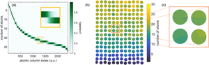
Fig. 2. Approach 1. A probability matrix (a) summarizes the probability for each atomic column's scattering cross-section to correspond to the different thicknesses. It is a different manner to display the estimated Gaussian mixture model, and can be used to represent the counting results using a scatter pie plot (b), rather than only showing the most likely counting result. (c) Magnified view of the pie charts used to statistically represent the counting results for each atomic column.

Fig. 3. Approach 2. (a) 95% prediction interval on the number of atoms for each atomic column of the simulated Au nanorod from Figure 1. (b) Sample distribution from which the 95% prediction interval was estimated. (c) Magnified view of the pie charts used to statistically represent the counting results for each atomic column.

Fig. 4. Approach 3. (a) ICL criterion with the region of interest for combining different models highlighted. The inset shows the weights used to average the different models. (b) Scatter pie plot showing the possible counting results by combining the different models for the example from Figure 1. (c) Magnified view of the pie charts used to statistically represent the counting results for each atomic column.
To this purpose, the distribution of the scattering cross-sections corresponding to atomic columns with the same number of atoms is modeled as a Gaussian distribution for each thickness  $g$ present in the sample (Van Aert et al., Reference Van Aert, Batenburg, Rossell, Erni and Van Tendeloo2011, Reference Van Aert, De Backer, Martinez, Goris, Bals, Van Tendeloo and Rosenauer2013; De Backer et al., Reference De Backer, Martinez, Rosenauer and Van Aert2013, Reference De Backer, Fatermans, den Dekker and Van Aert2021). Together, this results in a Gaussian mixture model with $G$ Gaussian components, where $G$ is the number of different thicknesses present in the sample. This is visualized in Figure 1c. More details can be found in the Appendix.
Due to the noise, it is impossible to accurately determine the correct number of components  $G$ based on a visual interpretation of the set of scattering cross-sections displayed in the histogram. Furthermore, this would be subjectively dependent on the chosen number of bins to represent the scattering cross-sections in the histogram. Therefore, an order selection criterion which balances the model likelihood against the model complexity is introduced to select the correct number of components $G$. Ideally, the true model order corresponds to a local minimum in the order selection criterion evaluated as a function of the number of components. The Integrated Classification Likelihood (ICL) criterion has been shown to have the best performance for atom-counting (De Backer et al., Reference De Backer, Martinez, Rosenauer and Van Aert2013) and is evaluated in Figure 1d. Multiple local minima can occur in the ICL criterion. The relevant local minimum can be selected by taking into account some prior knowledge about the system's geometry and/or sample thickness, or by comparing to image simulations, provided that the experimental images have been normalized with respect to the incident electron beam (De Backer et al., Reference De Backer, Martinez, Rosenauer and Van Aert2013; Jones, Reference Jones2016).
Next, counting results—shown in Figure 1e—are obtained by assigning the scattering cross-section of each atomic column to the component of the estimated probability distribution with the largest probability for this scattering cross-section. The precision of the counting results is, therefore, limited by the overlap between the Gaussian components. In this and all following visualizations of the counting results, a perpetually uniform, linear colormap from ColorCET was used (Kovesi, Reference Kovesi2015).
Approach 1: Showing the Inherent Uncertainty in the Gaussian Mixture Model
In fact, the counting result that is estimated using the statistics-based atom-counting is only the most likely counting result. By displaying this as the “true” estimate can be misleading in the sense that the feeling for the precision of the counting results is lost. This precision is, however, captured within the Gaussian mixture model, and is determined by the estimated width of the Gaussian components. Therefore, the first approach to present the counting results in a more representative manner, exploits all the information captured within the estimated Gaussian mixture model.
This can be done using a probability matrix, as shown in Figure 2a. The probability matrix summarizes the probability for each atomic column's scattering cross-section to correspond to the different thicknesses (De Backer et al., Reference De Backer, Van Aert, Nellist and Jones2022). This is further explained in the Appendix. In Figure 2, darker colors correspond to higher probabilities. In this representation, it becomes clear that some atomic columns are assigned a counting result with high probability. However, in many cases, the probabilities for assigning an atomic column to  $g$ or $g + 1$ atoms are similar, as visualized in the inset in Figure 2a. Especially, in these cases, it is useful to represent the counting results in a more statistical manner.
The representation chosen for this purpose is a scatter pie plot, where for each atomic column, the different possible thicknesses are visualized with their corresponding probability using a pie chart. The result is shown in Figure 2b for the atomic columns of the simulated Au rod indicated by the black box in Figure 1e. To allow a straightforward visual comparison, the counts are represented on the same color scale as the results shown for the next two approaches for this simulated Au nanorod. Note that both representations—probability matrix and scatter pie plot—in fact, contain the same information, but with the spatial context represented differently: via an arbitrary atomic column index or via the estimated atomic column positions, respectively. Visualizing the probabilities linked to the atomic column positions makes this approach especially useful in order to gain more insight in the counting uncertainty.
Approach 2: Sampling the Actual Distribution of the Atom Counts
The approach described in the previous section shows the uncertainty quantified by the width of the Gaussian components of the estimated Gaussian mixture model. Importantly, there is also uncertainty on the estimated parameters of the Gaussian mixture model. Therefore, we propose an approach based on sampling the actual distribution of the atom counts via noise realizations.
The starting point of this approach are the most likely counts, together with the average scattering cross-sections and the width of the Gaussian components of the estimated Gaussian mixture model. A noise realization is then generated by performing a random draw, for each atomic column, from the Gaussian distribution corresponding to the estimated most likely number of atoms. It was previously shown that the width of the Gaussian mixture model can be underestimated in some cases (De Backer et al., Reference De Backer, Martinez, Rosenauer and Van Aert2013). Therefore, in order to avoid inaccuracies in the set of noise realizations due to underestimation of the width of the Gaussian components in the initial analysis, the maximum of the estimated width  $\sigma$ and the dose-dependent width $\sigma _D = \mu _g/D$ was used, with $\mu _g$ the estimated average scattering cross-section corresponding to the $g$th component and $D$ the electron dose (Van Aert et al., Reference Van Aert, De Backer, Jones, Martinez, Béché and Nellist2019). From a specific noise realization, we obtain a new set of scattering cross-sections, corresponding to the estimated model. This set of scattering cross-sections is then analyzed using the statistical framework as previously described in the introduction to statistics-based atom-counting. Note that this implies that also for each noise realization the ICL criterion is evaluated to select the relevant number of components $G$. The set of most likely counting results for many of these noise realizations then constitute the sample distribution of the atom counts. This is a bootstrap procedure to quantify the uncertainty in the estimation process.
Based on this bootstrap sample distribution, a 95% prediction interval can be constructed for each atomic column, without any assumption on the type of distribution underlying the sample counting results (Geisser, Reference Geisser1993). The prediction interval for a given atomic column is obtained by ranking the estimated counts from the  $M$ different noise realizations for that atomic column in ascending order. The 95% prediction interval is chosen such that it is centered around the median of the estimated counts from the noise realizations. The lower bound and upper bound of the interval are then given by the estimated counts for the noise realizations that are the first and last, respectively, of $m$ realizations that fall within the range of the prediction interval. This range is chosen such that ${( m-1) }/{( M + 1) } = 95\percnt$. In this manner, the next counting result has a probability of 95% to fall within this prediction interval.
The interval is visualized in Figure 3a for the atomic columns of the simulated Au rod indicated by the black box in Figure 1e and provides a range within which the true number of atoms is expected to fall. This prediction interval was obtained based on 50 noise realizations. In this manner, it provides a clear and quantitative visualization of the uncertainty on the counting results. Note that the range of this prediction interval is rather large in this case, due to the low electron dose and high confidence level of 95%.
However, the different thicknesses enclosed by the prediction interval are not equally likely to correspond to the true thickness. Therefore, as an alternative representation, the whole sample distribution can be visualized for each atomic column using a pie chart, similar in interpretation to the results shown in the previous section for the first approach. This is shown in Figure 3b. Note that the information on the absolute range of possible counting results is the same in both representations for each atomic column. However, the scatter pie plot shows more nuance in the probability distribution over the different options to be considered, as compared with the wide prediction interval representation of Figure 3a.
In order to validate this second approach for representing the uncertainty on the atom-counting results, nested noise realizations were performed. The starting point was a ground truth number of atoms known from the structure of the simulated Au nanorod of Figure 1. The first set of 30 noise realizations serves to mimic the range that can be present in any experiment in case the ground truth is unknown. Based on each noise realization, a new set of 50 noise realizations was created based on the parameter estimates and counts. Each noise realization of this second set is then analyzed to obtain counting results that form a sample distribution for the counting results corresponding to the initial noise realization. The final goal of this analysis is to confirm whether the initial ground truth number of atoms is included in the final sample distribution, starting from an estimated Gaussian mixture model. We conclude that this second approach is indeed a reliable manner to achieve a statistical representation of the counting results, since the average percentage of atomic columns for which the true number of atoms falls within the 95% prediction interval—obtained based on 50 noise realizations—is expected to fluctuate around 95%, and was estimated equal to 99% for this set of only 30 noise realizations corresponding to an incident electron dose of  $10^{3}$ ${\rm e}^{-}/\mathring{\rm A}^{2}$.
Approach 3: Tackling Uncertainty in the Selection Criterion Based on the Concept of Model Averaging
The two approaches presented so far in fact assume that the selected local minimum from the order selection criterion corresponds to the correct model. In some situations, however, this assumption becomes difficult to justify objectively. The ICL criterion can present itself with a very shallow local minimum, where the values for  $G$ or $G + 1$ components are barely significantly different, making it impossible to reliably distinguish between those models. In this situation, the concept of model averaging can be a solution (Burnham & Anderson, Reference Burnham and Anderson2002).
Instead of selecting a single best model, it is argued that there is also an uncertainty in the model selection process. Therefore, results from multiple models are combined. In order to combine the different models, first a range of possible component numbers is selected, as indicated by the highlighted region in Figure 4a. The ICL values for these component numbers determine the weights with which the different models are combined, as follows:
 $$w_G = {\exp[ -( {1}/{c}) ( ICL( G) - \min_{F = G_i, \ldots, G_f}( ICL( F) ) ) ] \over \sum_{H = G_i}^{G_f} \exp[ -( {1}/{c}) ( ICL( H) - \min_{F = G_i, \ldots, G_f}( ICL( F) ) ) ] },\; $$
with  $w_G$ the weight for the model corresponding to $G$ components, while considering the models from $G_i$ until $G_f$ components. This equation was based on the expression given for an Akaike Information Criterion (AIC) from (Claeskens, Reference Claeskens2016). The factor 2 has been changed to a scaling parameter $c$, chosen equal to the minimum difference between subsequent ICL values in the considered range. The value of the ICL criterion at $G$ components, ${\rm ICL}( G)$, is calculated according to equation (A.6) of the Appendix.
The weights for the selected region are shown in the inset of Figure 4a. The most likely counting results following from the different models are then joined for each atomic column, according to the weights from equation (1). The (weighted) proportions for the different possible thicknesses obtained in this manner, then provides us with a statistical representation for the atom-counts. This is shown using a scatter pie plot in Figure 4b for the atomic columns of the simulated Au rod indicated by the black box in Figure 1e.
Discussion Using an Experimental Example
In order to compare and discuss the three proposed approaches in more detail, they are applied to the quantification of an experimental ADF STEM image of an Au nanorod, shown in Figure 5a. The image was taken at an aberration-corrected ThermoFisher Scientific Titan operated at 300 kV, using a probe convergence angle of 20 mrad and detector collection angles 115–157 mrad. The incident electron dose used to acquire the image was  $5.5 \times 10^{4}\, {\rm e}^{-}/\mathring{\rm A}^{2}$. The results obtained via the conventional procedure for atom-counting are shown in Figures 5b, 5c, while the results of the three approaches presented in this paper are shown for comparison in Figures 5d–5f.

Fig. 5. (a) Experimental ADF STEM image of an Au nanorod. (b) Most likely counting results obtained using the conventional statistics-based atom-counting approach. (c) Enlarged view of the most likely counting results. (d–f) Scatter pie plots corresponding to the same enlarged area, obtained using the three approaches for statistically representing the counting results. Additionally, further magnified views of the pie charts used to statistically represent the counting results for each atomic column are shown. All counting results are presented using the same color scale, indicated in (b).
It is clear that the three approaches yield different statistical representations of the uncertainty on the estimated counting results. This is to be expected and can be explained since the three approaches account for statistical uncertainty at a different level. In the first approach, only the uncertainty on the assignment of the counting result to one of the estimated Gaussian components is evaluated. In the second approach, the fluctuation of the estimated model at a given number of components itself is simulated. Finally, in the third approach, several models are combined, to account for uncertainty within the ICL order selection criterion.
The first approach is the most straightforward and least computationally expensive. However, the uncertainty presented in this manner is usually limited to  ${\pm }1$, as can be seen from the rather small color variation in Figure 5d. The second approach covers a larger variation in the final atom-counts, but is also more computationally expensive, since it requires repeated creation and analysis of noise realizations based on the estimated model. This approach is especially useful when the number of atomic columns per thickness is small, since in this case it is more challenging to reliably estimate the model parameters correctly (De Backer et al., Reference De Backer, Martinez, Rosenauer and Van Aert2013).
In this second approach, we implicitly assume that the one model selected from the ICL order selection criterion to base these noise realizations on, can correspond to a correct model. For the experimental example discussed in this section, however, the ICL criterion exhibits a very shallow valley-like local minimum, as shown in Figure 6a. The local minimum occurs at  $G = 47$ components, but the ICL value for 44 components until 49 components are similar. A good match with simulations—within a range of 5%, which is a reasonable deviation for a small amount of sample tilt or a slightly mismeasured inner detector angle (De wael et al., Reference De wael, De Backer, Jones, Nellist and Van Aert2017)—could be found for 44 components until 48 components, as shown in Figure 6b. Therefore, this is the range considered for combining the different models, as indicated by the highlighted region in Figure 6a. The inset of Figure 6a shows the corresponding weights, determined using equation (1), used to obtain the result visualized in Figure 5f. Note that the agreement between the estimated locations—i.e., the average scattering cross-sections—for the different models and the library of simulated scattering cross-sections is achieved by including an offset. This means that the first component estimated by the Gaussian mixture model does not correspond to a set of atomic columns with 1 atom thickness, but with a higher number of atoms.

Fig. 6. (a) ICL criterion for the experimental ADF STEM image from Figure 5a. The highlighted region indicates the models considered for weighting the different models, according to the weights shown in the inset. (b) Scattering cross-sections as a function of thickness for the different models which are combined. The considered models have an agreement between the estimated and simulated scattering cross-sections within 5%.
Conclusion
The conventional representation of the atom-counts obtained from the statistics-based atom-counting procedure, shows the most likely estimated counts. However, this representation neglects unavoidable uncertainties in the atom-counting results. In reality, there is variability on the estimated counting results. This variability can have different origins: uncertainty within the estimated Gaussian mixture model, uncertainty on the estimated model parameters, or even uncertainty on the order of the Gaussian mixture model itself. This paper introduces three approaches that each deal with a different source of variability, and statistically represent the counting results.
The most obvious uncertainty is inherent to the Gaussian mixture model, since the Gaussian components have a finite width and overlap each other. This uncertainty on the assigned number of atoms can be represented using the first approach described in this paper. In this manner, the advantage of the statistical framework for atom-counting—a quantification of the counting precision—is explicitly shown. Of the three approaches presented in this paper, this first approach is the least computationally expensive. It does not provide a full view of the uncertainty present in the estimated model, but already significantly improves upon reporting the counting results as a point estimate.
The second approach presented here, improves upon this first approach, by simulating the uncertainty on the estimated model parameters using noise realizations, which is the goal of the second approach discussed in this paper. By generating a new set of scattering cross-sections based on the estimated parameters, and consecutively analyzing that set of scattering cross-sections again using the statistics-based method for atom-counting, including model order selection, we achieve a sample distribution representative of the actual number of atoms in each atomic column. From this sample distribution, an interval can be estimated, rather than a point estimate.
Another situation that can occur is that the order selection criterion is especially unclear. Different options for the number of components can yield similar values in the criterion. In this case, an important source of variability on the counting results is the model order. The concept of model averaging is an ideal technique for dealing with this type of uncertainty. In this case, the weighted average of the counting results of models with different orders that can not be significantly distinguished is used to represent the uncertainty on the atom-counting results. In principle, approaches 2 and 3 could also be combined to account for the various types of uncertainty on the estimated results at the same time. This could be especially relevant in case the lowest or highest model order considered when combining the different models corresponds to the actual underlying model. Note that the third approach is not especially relevant in case of an order selection criterion that has a very pronounced local minimum. In those cases, the selection of the number of components is not the largest source of uncertainty, and approaches 1 or 2 are more appropriate.
With these three approaches, this paper aims to be a first step toward an even more statistical representation of the atom-counting results from ADF STEM images.
Acknowledgments
This project has received funding from the European Research Council (ERC) under the European Union's Horizon 2020 research and innovation programme (Grant Agreement No. 770887 and No. 823717 ESTEEM3). The authors acknowledge financial support from the Research Foundation Flanders (FWO, Belgium) through grants to A.D.w. and A.D.B. and projects G.0502.18N, G.0267.18N, and EOS 30489208. S.V.A. acknowledges TOP BOF funding from the University of Antwerp. The authors are grateful to L.M. Liz-Marzán (CIC biomaGUNE and Ikerbasque) for providing the samples.
Conflict of interest
The authors declare that they have no competing interest.
Appendix
Gaussian Mixture Model
The distribution of the scattering cross-sections corresponding to atomic columns with the same number of atoms can be modeled as a Gaussian distribution for each thickness  $g$ present in the sample (Van Aert et al., Reference Van Aert, Batenburg, Rossell, Erni and Van Tendeloo2011, Reference Van Aert, De Backer, Martinez, Goris, Bals, Van Tendeloo and Rosenauer2013; De Backer et al., Reference De Backer, Martinez, Rosenauer and Van Aert2013, Reference De Backer, Fatermans, den Dekker and Van Aert2021). Together, this results in a Gaussian mixture model with $G$ Gaussian components, where $G$ is the number of different thicknesses present in the sample. The Gaussian mixture model is given by:
 $$f_{{\rm mix}}\left(V_n\, \vert \, {\bf \Psi}_G\right) = \sum_{g = 1}^{G} \pi_g {\cal N}\left(V_n\, \vert \, \mu_g,\; \sigma\right),\; $$
with
 $${\cal N}\left(V_n\, \vert \, \mu_g,\; \sigma\right) = {1\over \sqrt{2\pi}\sigma} \exp\left(-{( V_n - \mu_g) ^{2}\over 2\sigma^{2}} \right),\; $$
the Gaussian components, visualized in Figure 1c.
In these expressions,  $\mu _g$ represents the location, i.e., the average scattering cross-section value, of the $g$th component in the mixture model and $\sigma$ represents the width of the components, while $V_n$ represents the stochastic variable related to the $n$th scattering cross-section. The stochastic variables for all scattering cross-sections are summarized in the vector ${\bf V}$. The mixing proportion $\pi _g$ of the $g$th component indicates which fraction of the columns in the image have a specific number of atoms corresponding to the $g$th component, i.e., the weight of the $g$th component in the Gaussian mixture model. The vector ${\bf \Psi }_G$ is the parameter vector containing all unknown parameters to be estimated in a Gaussian mixture model with $G$ components:
 $${\bf \Psi}_G = ( \pi_1,\; \ldots,\; \pi_{G-1},\; \mu_1,\; \ldots,\; \mu_G,\; \sigma) ^{\sf T }.$$
The joint probability density function of all scattering cross-sections is obtained starting from the Gaussian mixture model of equation (A.1) by taking the product over all atomic columns  $n$, since the scattering cross-sections are independent from each other:
 $$p( {\bf V}\, \vert \, {\bf \Psi}_G) = \prod_{n = 1}^{N} \sum_{g = 1}^{G} \pi_g {\cal N}\left(V_n\, \vert \, \mu_g,\; \sigma\right).$$
 The parameters  ${\bf \Psi }_G$ of the probability distribution of the scattering cross-sections are estimated, by maximizing the likelihood function. The expression for the likelihood function has the same functional form as the joint probability density function, but is evaluated as a function of the parameters rather than as a function of the stochastic variables related to the observed data. Specifically for this expression, the observed scattering cross-sections $\hat {{\bf V}}$ are inserted:
 $$L( {\bf \Psi}^{\rm stat}_G) = p( \hat{{\bf V}}\, \vert \, {\bf \Psi}^{\rm stat}_G) = \prod_{n = 1}^{N} f_{{\rm mix}}\left(\hat{V}_n\, \vert \, {\bf \Psi}^{\rm stat}_G\right).$$
The parameter estimates are iteratively calculated using the expectation maximization (EM) algorithm (Dempster et al., Reference Dempster, Laird and Rubin1977).
ICL Criterion
So far, we have considered the estimation of the probability distribution of the scattered intensities presuming a specific number of components  $G$. However, due to the noise, it is impossible to accurately determine the correct number of components based on a visual interpretation of the set of scattering cross-sections displayed in the histogram. Furthermore, this would be subjectively dependent on the chosen number of bins to represent the scattering cross-sections in the histogram. Therefore, an order selection criterion which balances the model likelihood against the model complexity is introduced to select the correct number of components $G$. The model order corresponds to a local minimum in the order selection criterion evaluated as a function of the number of components. Many different information criteria exist (McLachlan & Peel, Reference McLachlan and Peel2000), but the Integrated Classification Likelihood (ICL) criterion (Biernacki et al., Reference Biernacki, Celeux and Govaert2000) has been shown to have the best performance for atom-counting (De Backer et al., Reference De Backer, Martinez, Rosenauer and Van Aert2013). The ICL criterion is expressed as follows:
 $${\rm ICL}( G) = -2 \log L( {\hat{\bf \Psi}}_G) + 2 {\rm EN}( \hat{\tau}) + d \log N,\; $$
with  $-2 \log L( {\hat {\bf \Psi }}_G)$ the likelihood term depending on the estimated parameters ${\hat {\bf \Psi }}_G$ and $2{\rm EN}( \hat {\tau }) + d \log N$ the penalty term depending on the sample size $N$, the number of parameters $d = 2G$ and an entropy term:
 $${\rm EN}( \hat{\tau}) = - \sum_{g = 1}^{G} \sum_{n = 1}^{N} \tau_g \left(\hat{V}_n \, \vert \, {\hat{\bf \Psi}}_G \right)\log \tau_g\left(\hat{V}_n \, \vert \, {\hat{\bf \Psi}}_G \right),\; $$
with  $\tau _g( \hat {V}_n \, \vert \, {\hat {\bf \Psi }}_G )$ the posterior probability that the estimated scattering cross-section of the $n$th column $\hat {V}_n$ belongs to the $g$th component. This entropy term favors mixture models with well-separated components, in order to estimate physically relevant Gaussian mixture models.
Probability Matrix
A different manner of representing the estimated Gaussian mixture model from equation (A.1) is by using a probability matrix. This matrix summarizes the posterior probability for each atomic column's scattering cross-section to correspond to the different thicknesses. This can be understood via the Bayes’ theorem, as also discussed in De Backer et al. (Reference De Backer, Van Aert, Nellist and Jones2022):
 $$p\left(g\, \vert \, \hat{V}_n\right) = {\,p\left(g \right)p\left(\hat{V}_n \, \vert \, g \right)\over \sum_{h = 1}^{G} p \left(h\right)p\left(\hat{V}_n \, \vert \, h \right)},\; $$
 $$ = {\hat{\pi}_g {\cal N}\left(\hat{V}_n \, \vert \, \hat{\mu}_g,\; \hat{\sigma}\right)\over \sum_{h = 1}^{G} \hat{\pi}_h {\cal N}\left(\hat{V}_n \, \vert \, \hat{\mu}_h,\; \hat{\sigma}\right)},\; \hskip -4pc $$
 $$= \tau_g\left(\hat{V}_n\, \vert \, {\hat{\bf \Psi}}_G\right).$$
An example of such a probability matrix is shown in Figure 2a, where  $p( g\, \vert \, \hat {V}_n)$ is evaluated for all possible thicknesses $g$ and for all atomic columns $n$.
$n$.


 Open access