


Introduction
“Thin films” are stratified materials and find tremendous applications in modern technology (e.g., electronic semiconductor devices, LEDs, magnetic recording media, optical coatings, and coatings on cutting tools). Accurate determination of the chemical composition of sub-micrometer to nanometer layers, however, requires special equipment/technique (Llovet et al., Reference Llovet, Moy, Pinard and Fournelle2021). The electron probe was not designed to analyze thin films, as the conventional matrix correction assumes a homogenous analytical volume. However, using the ingenuity of Castaing (Reference Castaing1951), the electron probe microanalysis (EPMA) technique has been used to determine the thickness and composition of layered specimens since the early 1960s (Sweeney et al., Reference Sweeney, Seebold and Birks1960; Llovet et al., Reference Llovet, Moy, Pinard and Fournelle2021). The method is employed in a wide variety of fields to determine, for example, coating thicknesses, oxidation layers, or thin-film homogeneity (Dumelié et al., Reference Dumelié, Benhayoune and Balossier2007). The method has been drastically improved since the 1990s with the development of realistic and accurate analytical descriptions of the depth distribution of the primary ionizations generated per incident electrons in the target: the ϕ(ρz) (phi-rho-z) distribution. Several ϕ(ρz) models exist: the models of Pouchou and Pichoir, PAP and XPPFootnote 1 (Pouchou & Pichoir, Reference Pouchou, Pichoir, Heinrich and Newbury1991), and the model of Merlet, XPHI (Merlet, Reference Merlet1995; Llovet & Merlet, Reference Llovet and Merlet2010) being the most recent ones developed and used most frequently. The ϕ(ρz) distribution is also commonly used to determine the composition of bulk samples, that is, having a thickness of at least several micrometers (depending on the studied material and the characteristic X-ray transition being evaluated). For a complete review of the existing ϕ(ρz) models used for bulk analysis, see Lavrent'ev et al. (Reference Lavrent'ev, Korolyuk and Usova2004).
In the case of layered specimens, the determination of the composition and thickness of the surface layer, of a buried layer, or of the substrate cannot be done using the traditional EPMA method and software. Special procedures and programs have to be employed. The most commonly used method is the multi-voltage analysis method which consists of the measurement of the k-ratios—the ratio of the X-ray intensity (corrected from the background and the dead-time) emitted by the studied element measured on the unknown and on a standard—at several accelerating voltages. The k-ratios are then compared with theoretical k-ratios calculated using a ϕ(ρz) model appropriate for thin-film determination and in which the thickness and/or the composition of the layers or substrate are the unknowns. The thicknesses and compositions are calculated by successive iterations on those values until the theoretical and experimental k-ratios are closely matched. Theoretically, in the simple case where no elements are simultaneously present in different layers, convergence can be achieved with only one set of k-ratios measured at a single accelerating voltage value, but in practice, several accelerating voltages are required to minimize the errors due to uncertainties on the k-ratio measurements and inaccuracies of the ϕ(ρz) model. This analysis procedure requires dedicated programs, and few labs appear to have thin-film analysis software. With exception of one of them, these programs are generally moderately expensive, and they may be difficult to afford for laboratories having only occasional requests to analyze stratified samples. One of the most frequently used free thin film analysis software programs is GMRFILM, a research-grade shareware DOS program created in the late 1980s by R. Waldo at General Motors Research (Waldo, Reference Waldo and Newbury1988). Despite its great capabilities, this program suffers from its age and modern operating systems do not readily support it anymore, making its use more complicated. The program also only allows the analysis of k-ratios measured at one accelerating voltage at a time, losing the benefits of the multi-voltage analysis. Most of the thin-film analysis programs are not open source, making them “black boxes” where it may be difficult to understand the internal computation sometimes needed to evaluate the credibility of the results.
To remedy the lack of freely available thin-film analysis software, this paper presents a new modern thin-film analysis program with a simple graphical user interface, BadgerFilm. To determine the layer thicknesses and compositions, the program uses the PAP ϕ(ρz) distribution described in Pouchou & Pichoir (Reference Pouchou, Pichoir, Heinrich and Newbury1991), as well as a nonlinear fitting procedure based on the Levenberg–Marquardt algorithm (Levenberg, Reference Levenberg1944; Marquardt, Reference Marquardt1963). This minimization algorithm generally finds a solution even if it starts very far from the final result, avoiding the need of accurate initial guesses. In addition, BadgerFilm implements algorithms for the calculation of secondary fluorescence by characteristic X-rays and bremsstrahlung, and uses some of the most recent atomic parameters such as the mass absorption coefficients (MACs), and the electron impact ionization cross sections to calculate absolute X-ray intensities (for an independent check against Monte Carlo simulations). BadgerFilm is written in .NET Visual Basic, is open source and can be freely downloaded at this address: https://github.com/Aurelien354/BadgerFilm.
Implemented Models
The foundation of the film analysis method by EPMA used in this work is based on the accurate analytical description of the ionization depth distribution by primary electron impact, the ϕ(ρz) distribution. This distribution is used to calculate the primary X-ray intensity, as well as the secondary fluorescence generated by the characteristic X-rays and, to a lesser extent, by the bremsstrahlung.
Primary Characteristic X-Ray Intensity
The primary X-ray intensity emitted from the sample is calculated using the PAP ϕ(ρz) ionization depth distribution as described by Pouchou & Pichoir (Reference Pouchou, Pichoir, Heinrich and Newbury1991). The properties of this model for bulk samples are described in a companion paper, Moy & Fournelle (Reference Moy and Fournelle2020).
In the case of multilayered samples, the primary X-ray intensity  $I_i^s$ emitted by the element i in the layer s located from mass depth ρzs to ρzs +1 is given by:
 $$I_i^s = n_{{\rm el}}{\rm \;}\displaystyle{{N_{\rm A}} \over {A_i}}\;C_i\;\omega _j\;\displaystyle{{{\rm \Gamma }_{\,j-k}} \over {{\rm \Gamma }_{\,j-{\rm total}}}}\;\lambda _j\;{\rm \sigma }_j\lpar {E_0} \rpar \;T_i^s \int_{\rho z_s}^{\rho z_{s + 1}} {\phi _j\lpar {\rho z} \rpar \hbox{e}^{\ndash {\rm \;\chi }_i^s {\rm \;}\lpar {\rho z-\rho z_s} \rpar }\;d\rho z\;\varepsilon \;\displaystyle{{\rm \Omega } \over {4\pi }}} $$
where n el is the number of incident electrons impinging the sample per second, N A is Avogadro's number, A i is the atomic weight of element i, C i is the weight fraction of element i, ω j is the fluorescence yield of shell (or subshell) j, the term Γj−k represents the radiative transition probability for an electron to make a transition from shell (or subshell) k to shell (or subshell) j, Γj−total is the total radiative width for all possible transitions to the j shell (or subshell), λ j is the enhancement factor which accounts for the fact that electron vacancies can be created in the considered shell by direct electron impact, but also by the migration of vacancies between subshells of the same shell through nonradiative transitions (Coster–Kronig and super-Coster–Kronig transitions), and between subshells of different, most inner, shells through radiative and nonradiative transitions (Llovet et al., Reference Llovet, Powell, Salvat and Jablonski2014). σ j(E 0) is the ionization cross section of the shell (or subshell) j by electron impact of incident energy E 0. ε and Ω/4π are the intrinsic detection efficiency and the solid angle of collection of the detector, respectively. The term 1/4π comes from the fact that the characteristic X-rays are emitted in 4π steradians (the X-ray emission is assumed to be isotropic).  $T_i^s$ represents the absorption of the emitted characteristic X-rays by the l layers above the considered layer s:
 $$T_i^s = \mathop \prod \limits_{l = 1}^{s-1} \hbox{e}^{-{\rm \chi }_i^l \;\lpar {\rho z_l-\rho z_{l-1}} \rpar }$$
 The term  ${\rm \chi }_i^l$ is the reduced MAC:
 $${\rm \chi }_i^l = \left({\displaystyle{\mu \over \rho }} \right)_i^l \;\displaystyle{1 \over {\sin \theta }}$$
where  $\lpar {\mu /\rho } \rpar _i^l$ is the MAC of the material for the studied radiation produced by the element i and absorbed in layer l, and θ is the takeoff angle of the detector. The term ρz l − ρz l−1 corresponds to the mass thickness of layer l. The term $e^{\ndash {\rm \;\chi }_i^s {\rm \;}\lpar {\rho z-\rho z_s} \rpar }$ represents the absorption of primary characteristic X-rays in the layer (or substrate) s where they were generated. This term is then integrated, analytically or numerically, over the mass thickness of the layer (or substrate) to obtain the total emitted X-ray intensity (up to a constant multiplier). The following distinction should be emphasized: the term $\phi _j\lpar {\rho z} \rpar \hbox{e}^{\ndash {\rm \;\chi }_i^s {\rm \;}\lpar {\rho z-\rho z_s} \rpar }$ is proportional to the emitted X-ray distribution, while the term ϕ j(ρz) is proportional to the generated X-ray distribution (see Fig. 1).

Fig. 1. Representation of the ϕ(ρz) distributions corresponding to the generated and emitted characteristic X-ray distribution for (a) the Si Kα X-ray line in pure bulk Si and (b) the B Kα X-ray line in bulk AlB2 (extremely high absorbing system), both at 10 kV. To calculate the emitted X-ray distribution, a takeoff angle of 40° was considered as well as MACs of 357.6 and 72,572 cm²/g for absorption of the Si Kα radiation by Si and for absorption of the B Kα radiation by AlB2, respectively. Results obtained with BadgerFilm.
It is worth noting that when calculating the k-ratio, that is, the ratio of the X-ray intensities measured on the unknown and on the standard at the same electron beam energy E 0, the electron impact ionization cross sections σ j(E 0) present outside of the ϕ(ρz) integral equation (1), as well as the relaxation parameters, cancel out between the numerator and the denominator.
In the case of layered or multilayered specimens, the ϕ(ρz) distribution in the film, and therefore the generated Kα X-ray distribution, is different from that of a bulk homogeneous specimen of the same material (see Fig. 2). Hence, the distribution must be modified to take into account the different perturbating effects, such as the backscattered electrons from one layer to another. In the PAP model, a weighting equation of the form p(ρz, L r, R r) = N(ρz − L r)2(ρz − R r)2 is used in order to generate sets of fictitious bulk compositions from which the form parameters of the ϕ(ρz) distribution [i.e., the ionization at the surface of the layer ϕ(0), the mass depth at which the ϕ(ρz) distribution is maximum R m, the maximum mass depth ionization R x, and the area of the ϕ(ρz) distribution F] are calculated (for more details, see Pouchou & Pichoir, Reference Pouchou, Pichoir, Heinrich and Newbury1991; Moy & Fournelle, Reference Moy and Fournelle2020). In this weighting law, L r and R r are the roots of the polynomial and usually vary between −R x and R x (Pouchou & Pichoir, Reference Pouchou, Pichoir, Heinrich and Newbury1991) and N is a normalization factor to ensure that the area of p(ρz, L r, R r) between 0 and R r is equal to 1. Based on the values of L r and R r, the polynomial function will give more or less weight to the first layer(s) of the stratified specimen allowing a better estimation of the form parameters. Different values of L r and R r are used to calculate the form parameters: (i) the first step is the calculation of R x using the root values R r = R x and L r = −0.4R x. As the values of R r and L r also depend on R x, the latter parameter is calculated in an iteration loop. The initial value of R x is calculated using a fictitious concentration  $C_i^f$ for the element i defined by $C_i^f = C_i/\sum\nolimits_k {C_k}$ where Ci is the real concentration of element i and the index k is running on all the elements composing the sample (film and substrate). Then, the weighting laws are applied to calculate a new set of fictitious concentrations and then a new value for R x. The iteration is stopped when the value of R x has varied less than 1% from the previous iteration. (ii) In a second step, root values of R r = 0.5R x and L r = −0.4R r are used to calculate the mean atomic number $\overline {Z_b}$ [calculated as $\overline {Z_b} = \left({\sum\nolimits_k {C_k^f Z_k^{0.5} } } \right)^2$ with Z k the atomic number of element k] in the formulation of the mean backscatter coefficient $\bar{\eta }$, which is in turn used for the calculation of the backscatter loss factor R involved in the determination of the area factor F, and the surface ionization ϕ(0) (see Pouchou & Pichoir, Reference Pouchou, Pichoir, Heinrich and Newbury1991; Moy & Fournelle, Reference Moy and Fournelle2020). These root values give more weight to the regions close to the surface of the sample. (iii) In a third step, roots of R r = 0.7R x and L r = −0.6R r are employed to calculate the mean atomic number $\bar{Z} = \sum\nolimits_k {C_k^f Z_k}$ used for the determination of the factors M and J in the calculation of the deceleration factor 1/S (see Pouchou & Pichoir, Reference Pouchou, Pichoir, Heinrich and Newbury1991; Moy & Fournelle, Reference Moy and Fournelle2020). (iv) In a fourth and final step, to calculate the mass depth R m corresponding to the maximum of the ϕ(ρz) distribution, a mean atomic number equals to $Z_{av} = \lpar {\overline {Z_b} + \bar{Z}} \rpar /2$ is used. At each step, using the weighting law with the appropriate root values, the fictitious compositions $C_i^f$ of the i elements constituting a given layer (or the substrate) are calculated by integration over the mass depth of the considered layer:
 $$C_i^f = C_i \times N \times \int_{\rho z_1}^{\rho z_2} {\,p\lpar {\rho z\comma \;L_r\comma \;R_r} \rpar \;d\rho z} $$
where ρz 1 and ρz 2 are the limits of the considered layer (or substrate) with the condition that ρz 2 should not exceed R x. Finally, all the fictitious compositions, from the layers and the substrate, are summed and normalized to 100 wt% to create a fictitious bulk sample that can be used to calculate the form parameters of the ϕ(ρz) distribution.
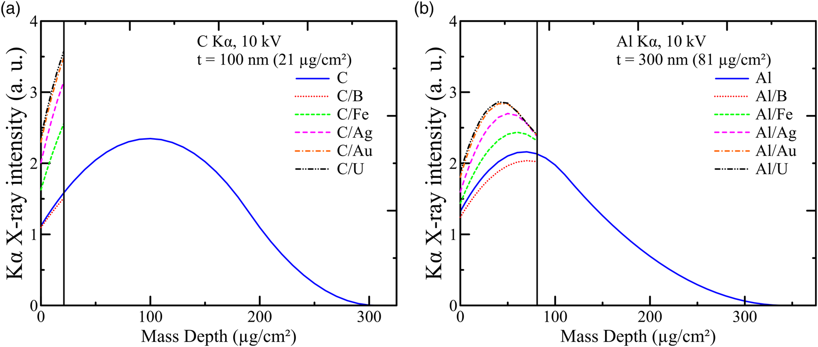
Fig. 2. Effects of the substrate material (B, Fe, Ag, Au, or U) on the generated Kα X-ray distribution in (a) a 100-nm-thick film of C and (b) a 300-nm-thick film of Al, at 10 kV. The higher the atomic number Z of the substrate, the higher the number of backscattered electrons into the film, leading to an increase of the ϕ(ρz) distribution in the film. Results obtained with BadgerFilm.
As an example, we consider a 100-nm-thick film of Al2O3 (52.93 wt% Al and 47.07 wt% O), with a density of 3.95 g/cm3, on top of a Cu substrate. The sample is examined at 15 kV, and the intensity of the Kα 1 X-ray line of the element Al is measured. The algorithm determines the ϕ(ρz) distribution for the thin film on the substrate by assuming that the film–substrate system is a bulk homogeneous sample. Table 1 reports the “equivalent” bulk elemental concentrations that would correspond to a 100-nm-thick Al2O3 film on Cu for the calculation of the different parameters of the ϕ(ρz) distribution. To calculate the parameter R x, an initial fictitious set of bulk concentrations is calculated by averaging the real concentrations without weighting law, giving an initial value for R x of 686.7 μg/cm² (see Table 1). Then, the weighting law is applied iteratively until convergence of R x to a value of 700.3 μg/cm². This value of R x is then used in the calculation of the next weighting laws (steps ii, iii, and iv previously described). As shown in Table 1, to determine the backscattered loss factor R and the surface ionization parameter ϕ(0), which are more dependent on the material compositions near the surface of the sample, the fictitious concentration of the elements constituting the film are enhanced by the weighting law. The fictitious composition of the sample used to calculate the parameters 1/S, and thus F thanks to R, lies in between the fictitious composition obtained to calculate the parameter R x, and the parameters R and ϕ(0).
Table 1. Fictitious Composition of a Bulk Al–Cu–O Sample and Model Parameters Used in the Determination of the ϕ(ρz) Distribution of a Film of Al2O3 (100 nm) Deposited on a Cu Substrate.

Data calculated for the Al Kα 1 X-ray line at 15 kV.
Secondary Fluorescence
In the following, we define the term fluorescence by the production of characteristic X-rays by other X-rays from the same phase. Similarly, we define the term secondary fluorescence as the production of characteristic X-rays by other characteristic X-rays (characteristic secondary fluorescence) or by X-rays from the continuum (bremsstrahlung secondary fluorescence) coming from another phase. In both bulk and multilayered samples, the fluorescence and secondary fluorescence effects can account for a nonnegligible part of the total produced X-rays. In the following, we describe the strategies employed to calculate the secondary fluorescence.
Characteristic Secondary Fluorescence
The determination of the secondary fluorescence created by characteristic X-rays requires the calculation of the ϕ(ρz) distribution integrated over the depth of the different layers of the specimen. Pouchou & Pichoir (Reference Pouchou, Pichoir, Heinrich and Newbury1991) used the XPP algorithm to predict the characteristic secondary fluorescence as this model is easier to integrate analytically and numerically. In our implementation, we instead use the full PAP algorithm to generate the characteristic secondary fluorescence [see Waldo (Reference Waldo and Howitt1991) and Supplementary Material for more details]. The phi-rho-z curves are used to calculate the depth distribution of generated characteristic X-rays, emitted in 4π steradian, which are then integrated along their path with the probability of ionizing the electron shell corresponding to the studied X-ray line in the layer of interest. The X-ray production rate is then calculated and integrated over the depth of the considered layer to calculate the X-ray emission rate. This last calculation takes into account the attenuation of the X-rays along their path to the surface of the sample, with a takeoff angle equals to the detector takeoff angle θ d (Fig. 3).

Fig. 3. Characteristic secondary fluorescence in a multilayer sample. The layer b made of material MB contains the element B that emits a characteristic X-ray of energy E 1 which will fluoresce element A of material MA in layer a, producing the studied characteristic X-ray of energy E 2.
For example, consider a characteristic X-ray of energy E 2 of element A located in the layer a between mass depth  $\rho _{M_A}z_a$ and $\rho _{M_A}z_{a + 1}$, being fluoresced by the characteristic X-rays of energy E 1 emitted by element B located in layer b between mass depth $\rho _{M_B}z_b$ and $\rho _{M_B}z_{b + 1}$. The secondary fluorescence of characteristic X-rays from element A produced by characteristic X-rays coming from element B is given by:
 $$\eqalign{I_i^s & = \int_{\pi /2}^\pi {\sin \lpar \theta \rpar \;n_{\rm el}\displaystyle{{N_{\rm A}} \over {A_B}}\;C_B\sigma _{e_m^- }^B \lpar {E_0} \rpar \lambda _m^B \;\omega _m^B \;\displaystyle{{{\rm \Gamma }_{m-n}^B } \over {{\rm \Gamma }_{m-{\rm total}}^B }}\;\times \displaystyle{1 \over {4\pi }}} \cr & \quad \times \int_{\rho _{M_B}z_b}^{\rho _{M_B}z_{b + 1}} {\phi _m^B \lpar {\rho_{M_B}z_0} \rpar \hbox{e}^{-{\lpar {\mu /\rho } \rpar }_{M_B}\lpar {E_1} \rpar \rho _{M_B}\lpar \lpar z_0-z_b \rpar/\cos \theta \rpar }d\rho _{M_B}z_0 \times \prod\limits_{k = b-1}^{a + 1} {{\rm e}^{-{\lpar {\mu /\rho } \rpar }_{M_k}\lpar {E_1} \rpar \rho _{M_k}\lpar t_k/\cos \theta \rpar }} } {\rm \;} \cr & \quad \times \int_{\rho _{M_A}z_{a + 1}}^{\rho _{M_A}z_a} {\hbox{e}^{-{\lpar {\mu /\rho } \rpar }_{M_A}\lpar {E_1} \rpar \rho _{M_A}\lpar \lpar z_{a + 1}-z \rpar/\cos \theta \rpar }\displaystyle{{N_{\rm A}} \over {A_A}}C_A\;\sigma _{\,ph_i}^A \lpar {E_1} \rpar \lambda _i^A \;\omega _i^A \;\displaystyle{{{\rm \Gamma }_{i-j}^A } \over {{\rm \Gamma }_{i-{\rm total}}^A }} \times \displaystyle{1 \over {4\pi }}\;} \cr & \quad \times \hbox{e}^{-{\lpar {\mu /\rho } \rpar }_{M_A}\lpar {E_2} \rpar \rho _{M_A}\lpar \lpar z-z_a \rpar /\sin \theta _d\rpar }\;\displaystyle{{d\rho _{M_A}z} \over {\cos \theta }}d\theta \prod\limits_{k = a-1}^0 {{\rm e}^{-{\lpar {\mu /\rho } \rpar }_{M_k}\lpar {E_2} \rpar \rho _{M_k}\lpar t_k/\sin \theta _d\rpar }2\pi \;\varepsilon \;{\rm \Omega }} } $$
 where  $\phi _m^B \lpar {\rho_{M_B}z_0} \rpar$ is the ionization depth distribution of electron shell (or subshell) m of element B present in the material M B at mass depth $\rho _{M_B}z_0$. The probability of producing an electron vacancy in the shell (or subshell) m by ionization is given by $\sigma _{e_m^- }^B \lpar {E_0} \rpar \lambda _m^B$ where $\sigma _{e_m^- }^B \lpar {E_0} \rpar$ and $\lambda _m^B$ are quantities previously defined and the superscript B indicates that these quantities belong to element B. A given characteristic X-ray of energy E 1 is emitted during the relaxation of the ionized atom B by transition of an electron from the shell n to the shell m. These are represented by the fluorescence yield $\omega _m^B$, the radiative transition probability for an electron to transition from shell n to shell m, ${\rm \Gamma }_{m-n}^B$, and the total radiative width for all possible transitions to the m shell, ${\rm \Gamma }_{m-{\rm total}}^B$. The characteristic X-rays of energy E 1 travel from layer b to layer a and undergo absorption along their path. The absorption of the photons, emitted with a direction θ, along their path in material M B is represented by the MAC $\lpar {\mu /\rho } \rpar _{M_B}\lpar {E_1} \rpar$ and taken into account by the exponential term $\hbox{e}^{-{\lpar {\mu /\rho } \rpar }_{M_B}\lpar {E_1} \rpar \rho _{M_B}\lpar \lpar z_0-z_b \rpar /\cos \theta \rpar }$. The product of the ionization depth distribution by the absorption exponential is integrated over the mass thickness of the layer b, from $\rho _{M_B}z_b$ to $\rho _{M_B}z_{b + 1}$. The photons exiting the layer b pass through the k layers between the layers a and b, of thicknesses t k and material M k, and undergo absorption taken into account by the MAC $\lpar {\mu /\rho } \rpar _{M_k}\lpar {E_1} \rpar$ and the thicknesses of each of the k layers tk. When the photons reach the layer a, the X-rays are then absorbed by the material M A, taken into account through the MAC $\lpar {\mu /\rho } \rpar _{M_A}\lpar {E_1} \rpar$. At mass depth $\rho _{M_A}z$, in the infinitely small distance ds, the probability for the X-rays to interact with the atoms of element A through photoelectric interaction and to ionize the electron shell i of element A is given by
 $$1-{\rm e}^{-\lpar \rho N_{\rm A}/A_A\rpar C_A{\rm \;}\sigma _{\,ph_i}^A \lpar {E_1} \rpar \lambda _i^A \;ds}\approx \displaystyle{{\rho N_{\rm A}} \over {A_A}}C_A{\rm \;}\sigma _{\,ph_i}^A \lpar {E_1} \rpar \lambda _i^A \;ds\comma \;$$
 where  $\sigma _{ph_i}^A \lpar {E_1} \rpar$ is the photoelectric cross section leading to an ionization in shell i of element A by interaction with a photon of energy E 1. The production of the studied characteristic X-ray of energy E 2 emitted by element A during the relaxation process from which an electron from the shell j falls into the shell i is taken into account by the fluorescence yield $\omega _i^A$ and radiation yields ${\rm \Gamma }_{i-j}^A$ and ${\rm \Gamma }_{i-{\rm total}}^A$. The attenuation of these X-rays, emitted toward the detector with an angle θ d, in the layer a itself and in the layers above the layer a, is taken into account by the exponentials with MACs $\lpar {\mu /\rho } \rpar _{M_A}\lpar {E_2} \rpar$ and $\lpar {\mu /\rho } \rpar _{M_k}\lpar {E_2} \rpar$, respectively. ε and Ω are the intrinsic detection efficiency and the solid angle of collection of the detector, respectively.
The analytical resolution of this equation is possible when using the PAP ionization distribution model. For more details on the resolution of this equation and for other cases (e.g., layer a below layer b), see Waldo (Reference Waldo and Howitt1991) and Supplementary Material.
Bremsstrahlung Secondary Fluorescence
The issue of secondary fluorescence created by the bremsstrahlung can be an important factor in correctly evaluating many thin films. Previously, it was treated with a simplistic assumption that all bremsstrahlung X-rays were produced at a point on the surface of the evaluated layer (Pouchou & Pichoir, Reference Pouchou, Pichoir, Heinrich and Newbury1991). Instead, here we use the method described in Moy & Fournelle (Reference Moy and Fournelle2020) which consists in creating a ϕ(ρz) distribution for each discrete energy of the spectrum by considering an “imaginary” element with a characteristic X-ray energy equals to the bremsstrahlung X-ray energy being considered. Then, for a given material composition and electron beam energy, we have a ϕ(ρz) distribution, φ Brem(ρz;Eph), which models the depth distribution of generated bremsstrahlung X-rays of energy E ph. Then, just as done for evaluating characteristic secondary fluorescence, these bremsstrahlung φ Brem(ρz;Eph) distributions are integrated over the total depth of the layered sample, giving the secondary fluorescence intensity created by the bremsstrahlung X-rays of energy Eph. This process is repeated for other bremsstrahlung X-ray energies Eph in the range from E c, the ionization threshold of the considered characteristic X-rays, up to E 0, to model the amount of bremsstrahlung secondary fluorescence as a function of the X-ray energy. The bremsstrahlung φ Brem(ρz;Eph) distribution, calculated using the PAP model and an imaginary element, however, is a rough approximation of the real bremsstrahlung distribution. These φ Brem(ρz;Eph) distributions lead to a bremsstrahlung energy spectrum that does not always accurately represent a realistic bremsstrahlung energy spectrum. In order to assist in correcting the differences—considering only X-rays produced by bremsstrahlung secondary fluorescence—the shape of the calculated bremsstrahlung spectrum is multiplied by the shape of the bremsstrahlung spectrum [spectral distribution I(E)] given by Small et al. (Reference Small, Leigh, Newbury and Myklebust1987) and modified by Kulenkampff (as cited in Pouchou & Pichoir, Reference Pouchou, Pichoir, Heinrich and Newbury1991). See Moy & Fournelle (Reference Moy and Fournelle2020) for more details on this correction. This method, which is more rigorous theoretically than the usual point surface simplification (which does not take into account the subsurface), seems to overestimate bremsstrahlung secondary fluorescence when compared with Monte Carlo simulations.
The calculated bremsstrahlung secondary fluorescence can be improved by introducing two empirical parameters: α which artificially modifies the primary electron energy and β which modifies the absolute value of Small et al.'s bremsstrahlung spectral distribution. The values of α and β were determined using PENEPMA (Llovet & Salvat, Reference Llovet and Salvat2017) Monte Carlo simulations, for pure elements using their Kα, Lα, and Mα X-ray lines. For each X-ray transition, the α and β values were fitted incrementally against the element's atomic number Z with a polynomial function, shown in Figure 4. Good coefficients of determination R² were obtained for most of the fitting functions except for the coefficient β for the Mα X-ray lines where a value of R² = 0.858 was obtained. These polynomials were then used in the BadgerFilm code to predict the bremsstrahlung secondary fluorescence. We note that the discontinuities for the Lα lines appear to correspond with the populating of the electron shells of the different elements. This behavior, though, is not observed for the Kα and Mα lines.

Fig. 4. α and β coefficients used to enhance the bremsstrahlung secondary fluorescence for the Kα, Lα, and Mα X-ray lines. The symbols were determined by fitting the coefficients to the results of Monte Carlo simulations. The continuous lines represent the fit of the determined coefficients over the atomic number Z.
BadgerFilm
We have implemented the algorithms described above in an open-source graphical user interface program called BadgerFilm, which can calculate thickness(es) and composition(s) of thin films as well as composition of the substrate. Users are able to easily set various parameters, such as composition(s) and layer thickness(es) if known, as well as the takeoff angle of the detector, the MAC dataset or the ionization cross section (Fig. 5). The experimental data—the element, X-ray line, experimental k-ratio, accelerating voltage(s), and uncertainty on the k-ratio—can be entered by the user either manually or by copy-paste operation. K-ratios may be defined either relative to a pure element standard or a compound reference material, which the user has previously set up in BadgerFilm. The following characteristic X-ray lines are considered in the calculations as potential sources of characteristic secondary fluorescence, with the condition that their energy is greater than the ionization threshold of the studied X-ray line: Kα 1, Kα 2, Kβ, Lα 1, Lα 2, Lβ 1, Lγ 1, Lη, Lℓ, L3N5, Mα 1, Mα 2, Mβ 1, Mγ 1, M4O6, M3O5, M2N4, M2N1, M3O1, M3O4, M1N2, M1N3, M2O4, and M1O2. The program uses a nonlinear fitting algorithm based upon the Levenberg–Marquardt fitting algorithm (Levenberg, Reference Levenberg1944; Marquardt, Reference Marquardt1963) to iterate comparisons of estimated k-ratios with the experimental k-ratios, by variation of the compositions and thicknesses of the films (and substrate if so set), until convergence. It should be noted that with the bremsstrahlung secondary fluorescence turned on, in rare cases, the program has been observed to fail to converge to a realistic solution because of numerical instabilities at low overvoltage.
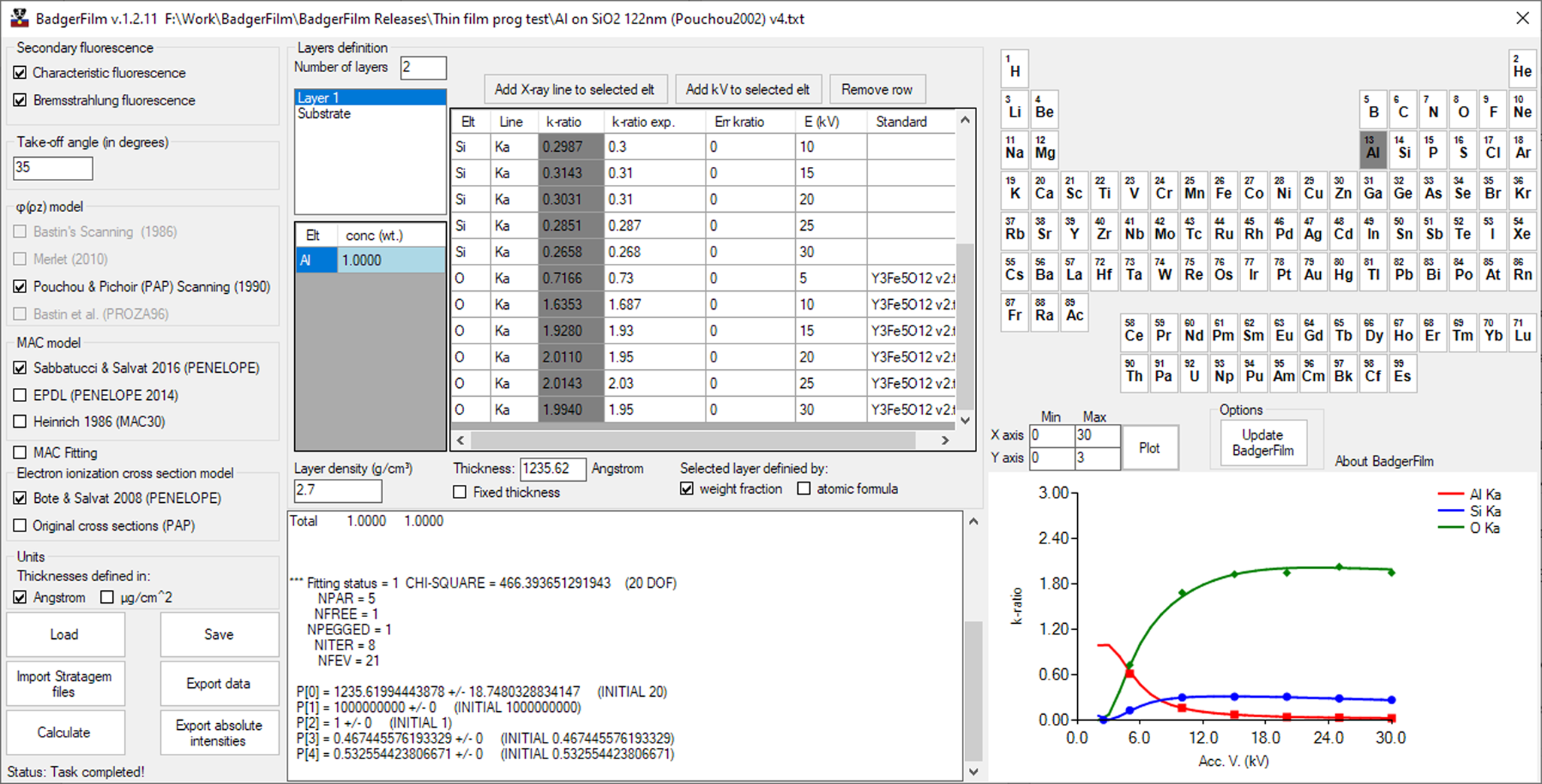
Fig. 5. BadgerFilm graphical user interface. The different options allow the users to easily analyze EPMA experimental data.
By default, the atomic parameters used in BadgerFilm (relaxation parameters, MACs, and ionization cross sections) to calculate the X-ray production rate are the same as those used in the PENELOPE 2018 (Salvat, Reference Salvat2019) database. PENELOPE 2018 is a general-purpose Monte Carlo code dedicated to the simulation of coupled electron-photon transport in arbitrary materials. This is an additional accuracy check and allows a direct comparison of the generated X-ray intensity between Monte Carlo simulations performed by PENEPMA (Llovet & Salvat, Reference Llovet and Salvat2017) and our implementation of the PAP algorithm. PENEPMA is a program dedicated to the simulation of X-ray spectra and quantities of interest for microanalysis by EPMA. It uses the subroutines of the Monte Carlo code PENELOPE (Salvat, Reference Salvat2019). The MACs employed by default in BadgerFilm have been extracted from PENELOPE 2018, which were calculated from the photoelectric cross sections of Sabbatucci & Salvat (Reference Sabbatucci and Salvat2016). The electron impact X-ray production cross sections were calculated using the electron impact ionization cross sections of Bote & Salvat (Reference Bote and Salvat2008) and the transition rates (fluorescence yields and radiation yields) extracted from the LLNL Evaluated Atomic Data Library (EADL) tables (Perkins et al., Reference Perkins, Cullen, Chen, Rathkopf, Scofield and Hubbell1991). For more details about the calculation of the X-ray production cross sections, see Moy et al. (Reference Moy, Merlet, Llovet and Dugne2013) and Moy & Fournelle (Reference Moy and Fournelle2020). Notice that the electron impact ionization cross sections used inside the PAP algorithm—based on the Hutchins model (Hutchins, Reference Hutchins, Kane and Larrabee1974)—and necessary to calculate the form factor F [the area of the ϕ(ρz) distribution] were not changed, as they are intrinsically related to the good performance of the model.
In addition, other atomic parameter models can be chosen to perform the calculations: the MAC model of Heinrich (Reference Heinrich, Brown and Packwood1987) or MACs calculated from the photoelectric cross sections extracted from the LLNL Evaluated Photon Data Library (EPDL97) (Cullen et al., Reference Cullen, Hubbell and Kissel1997). Particular MAC values can also be substituted by experimental values defined by the user (for a particular element and a particular X-ray line). Also, the ionization cross-section model of Hutchins (Reference Hutchins, Kane and Larrabee1974) can be chosen to perform the calculations.
The calculated results by BadgerFilm are displayed with an uncertainty estimate. These uncertainty estimates are based upon experimental k-ratio uncertainties—by default a value of 5% is set, unless user-specified, corresponding to an uncertainty on the measured X-ray intensities of 3.5% for both the unknown and the standard—which are propagated throughout the fitting algorithm. However, these uncertainties do not take into account uncertainties associated with the atomic parameters and with the ϕ(ρz) model (Ritchie & Newbury, Reference Ritchie and Newbury2012; Ritchie, Reference Ritchie2020). The user then can examine a visual graphical representation which shows both the experimental k-ratios plotted versus the accelerating voltage and the modeled best-fit solution. All of the input data can be saved in a BadgerFilm text file and easily reloaded later, if further manipulation of the parameters is required. The user may also import files in the STRATAGem (version 6.2) format, enabling compatibility with STRATAGem and Probe for EPMA (Donovan et al., Reference Donovan, Kremser, Fournelle and Goemann2020). All of the results from BadgerFilm can be easily exported to a spreadsheet program in a convenient format.
X-Ray Intensity Predictions: Comparison to Experimental Data and Monte Carlo Simulations
To demonstrate its accuracy, the implemented ϕ(ρz) calculation method should be validated against experimental measurements on bulk and thin-film samples of known composition(s) and thickness(es), when available. It is beneficial to not only compare the model's predictions to k-ratios, but full Monte Carlo simulations as it allows the comparison of absolute X-ray intensities. This permits the researcher to separate the primary X-ray intensity from the characteristic secondary fluorescence and from the bremsstrahlung secondary fluorescence (where the Monte Carlo program models that separation), allowing secondary fluorescence calculation algorithms to be validated. In this manner, BadgerFilm predictions were compared with X-ray intensities emitted from thin films and multilayered specimens.
PENEPMA (2018) was used to generate Monte Carlo simulations to compare with BadgerFilm results. PENEPMA's interaction mechanisms use scattering models that combine numerical tables with analytical cross-section models. The PENEPMA simulation algorithm is valid for energies from a few hundred electron volts to about 1 GeV (Salvat, Reference Salvat2019). Llovet & Merlet (Reference Llovet and Merlet2010) and Moy et al. (Reference Moy, Merlet and Dugne2015) demonstrated that PENEPMA yields good accuracy for absolute X-ray intensity values. X-ray intensity comparisons, between PENEPMA and BadgerFilm, were made for all three relevant X-ray intensities: for primary electron generated X-rays, for secondary fluorescence due to characteristic X-rays, and for secondary fluorescence due to the bremsstrahlung. These comparisons were made for all elements from C to Am, for beam energies from 5 to 30 kV and for Kα, Lα, Mα lines relevant to EPMA. [See our companion paper (Moy & Fournelle, Reference Moy and Fournelle2020) for discussion of the PAP ϕ(ρz) model used here and demonstration of its good performance when compared with experimental and Monte Carlo simulations for bulk materials.]
Thin Films
The predictions of the implemented model have been tested on different sets of data acquired on thin-film samples and available in the literature. In the following, experimental k-ratios were processed by our software's thin film algorithm using the PAP procedure, a correction for the secondary fluorescence produced by both the characteristic X-rays and the bremsstrahlung, the MACs extracted from PENELOPE 2018, and, to produce absolute X-ray intensities, the ionization cross sections of Bote & Salvat (Reference Bote and Salvat2008) and the relaxation parameters from the EADL tables (Perkins et al., Reference Perkins, Cullen, Chen, Rathkopf, Scofield and Hubbell1991). For comparison purposes, the k-ratios were also analyzed with the commercial software STRATAGem (STRATAGem version 6.2) using the PAP algorithm and including both characteristic and bremsstrahlung fluorescence contributions built into it, with the freely available DOS thin-film analysis code GMRfilm (Waldo, Reference Waldo and Newbury1988) and with the Monte Carlo code PENEPMA (Llovet & Salvat, Reference Llovet and Salvat2017).
Pouchou (Reference Pouchou2002) performed a series of measurements on a thin-film sample consisting of an Al film deposited on a SiO2 bulk substrate. The experimental k-ratios were measured at 5, 10, 15, 20, 25, and 30 kV using the Al Kα, Si Kα, and O Kα X-ray lines, and a takeoff angle of 35°. The standards used were pure Al, pure Si, and an yttrium iron garnet (Y3Fe5O12) standard for oxygen. The composition of the layer and substrate are assumed to be known, and only the film thickness was determined. Using STRATAGem and the XPP algorithm, Pouchou found a very good agreement of the theoretical k-ratios compared with the experimental ones using an Al mass thickness of ~30 μg/cm² (corresponding to an Al thin-film thickness of ~111 nm assuming an Al density of 2.7 g/cm3). The results given by BadgerFilm as well as version 6.2 of STRATAGem, GMRFilm, and PENEPMA are displayed in Figure 6. All the programs give very close thickness values, of about 122 nm in good agreement with the original publication of Pouchou. The predictions of BadgerFilm are in excellent agreement with the experimental data, reproducing very well the experimental k-ratios even for the lighter element oxygen. GMRFilm also gives results in excellent agreement with the experimental data. STRATAGem despite underestimating the k-ratios for the element oxygen, also gives very good predictions for the Al and Si k-ratios. Finally, PENEPMA seems to slightly overestimate the predicted k-ratios for O when using an Al film thickness of 122 nm. However, the k-ratios for the elements Al and Si are extremely well reproduced.

Fig. 6. Thickness determination of an Al film deposited on top of a SiO2 substrate using different calculation codes. Symbols are experimental k-ratios from Pouchou (Reference Pouchou2002). Continuous lines are the predictions of the analytical calculations. Open symbols linked by dashed lines are the predictions of Monte Carlo simulations (calculations were performed at the same accelerating voltages as the experimental measurements and linked by straight lines). In this simple case, the different methods give very similar thickness results.
In an earlier study, Pouchou (Reference Pouchou1993) determined the composition and thickness of a bilayer on a substrate specimen. The top layer is composed of Ni–Cr, the buried layer is composed of Fe, Gd, and Pt, and the substrate is made of pure Si. The sample was characterized by Rutherford backscattering (RBS) technique as well as by EPMA. The EPMA measurements were performed at 20, 25, and 30 kV, and the recorded X-ray lines were Ni Kα, Cr Kα, Fe Kα, Gd Lα, and Pt Mα. Pure standards were used to calculate the k-ratios that were then originally analyzed with the thin-film analysis code Strata, a precursor to the STRATAGem software. The experimental k-ratios have been re-analyzed with the PAP algorithm and secondary fluorescence included using GMRFilm, using only the measurements performed at 30 kV, using STRATAGem (version 6.2), and using BadgerFilm (Table 2). The uncertainty on the BadgerFilm results are uncertainties associated to the fitting procedure and obtained by assuming a 5% uncertainty on the experimental data. The thickness predictions of BadgerFilm are in very good agreement with the RBS measurements, especially for the top layer. The determined thickness of the second layer has a difference of 2% compared with the RBS measurements. The composition of the layers is also predicted very well by our program, with a highest deviation, compared with the RBS measurements, of 2.8% for the element Gd. BadgerFilm predictions also agree well with the results of the other programs. The fit to the experimental data is also very well reproduced as seen in Figure 7. This demonstrates the very good performance of BadgerFilm, and more generally of the PAP algorithm, to analyze multilayered specimens.
Table 2. Determination of the Compositions and Thicknesses of an Ni–Cr/Fe–Gd–Pt/Si Multilayer Specimen, From Pouchou (Reference Pouchou1993), by Different Techniques and Thin-Film Analysis Programs.

T refers to the thickness of the layers, in Angstroms.

Fig. 7. BadgerFilm fit of the Ni–Cr/Fe–Gd–Pt/Si experimental k-ratios. The thicknesses and compositions of the films were set as unknowns. The theoretical predictions for the calculated thicknesses and compositions match well the experimental measurements as displayed in Table 2.
BadgerFilm Applications
Ge Film on Ga–As
Thin films of Ge deposited on a Ga–As substrate were made at the Department of Chemical and Biological Engineering, University of Wisconsin-Madison. The samples were grown by slow vapor deposition (0.040 nm/s). The Ge layer is lattice matched to the Ga–As substrate and should not present any void area potentially affecting the density of the Ge layer. Two samples were made with two greatly different film thicknesses. The film thicknesses were first determined by X-ray reflectometry, and the obtained thicknesses were about 38 ± 2 and 320 ± 10 nm.
EPMA measurements were performed on both films using the CAMECA SXFive FE (CAMECA, Paris, France) microprobe located at the Eugene Cameron electron microprobe facility, Department of Geoscience, University of Wisconsin-Madison. X-ray intensities were recorded using wavelength-dispersive spectrometers at accelerating voltages of 5, 6, 7, 8, 9, 10, 13, 15, 20, 25, and 30 kV and with an electron beam Faraday cup current of 20 nA. The Lα X-ray lines of the elements Ga, Ge, and As were recorded as well as the Kα X-ray lines when available [the K shell ionization edge energies of Ga, Ge, and As are 10.367, 11.104, and 11.867 keV, respectively (Zschornack, Reference Zschornack2007)]. The Lα and Kα X-ray lines were measured using TAP (2d = 25.745 Å) and LLiF (2d = 4.0267 Å) monochromator crystals, respectively. The Kα X-ray line of C was also measured using an LPC2 (2d = 99.136 Å) crystal. This element was measured to determine the carbon coating thickness on top of the standards used to calculate the k-ratios (the thin-film samples were not coated). Even if Ge and As–Ga materials are conductive, these standards are part of a mount that contains conductive and nonconductive standards which are mounted in nonconductive epoxy. For this reason, the entire mount is carbon coated. The net X-ray intensity was determined by measuring the peak intensity for 10 seconds and the backgrounds on each side of the peak for 5 seconds. To calculate the k-ratios, standards of pure Ge and GaAs were used. The standards are on the same mount, and all are carbon coated. At each accelerating voltage, 5 points were acquired on each standard and 10 points on each thin film. Uncertainties on the k-ratios, Δk, were obtained by calculating the standard deviation of the measurements on the film samples and on the standards using the following formula:
 $${\rm \Delta }k = k \times \sqrt {{\left({\displaystyle{{{\rm \Delta }I_f} \over {I_f}}} \right)}^2 + {\left({\displaystyle{{{\rm \Delta }I_s} \over {I_s}}} \right)}^2} $$
where k is the calculated k-ratio, ΔI x and I x are the standard deviation and average X-ray intensity, respectively. The indices f and s denote the film and standard samples, respectively.
The experimental k-ratios were analyzed by BadgerFilm using the PAP matrix correction algorithm, and the MACs extracted from PENELOPE 2018. The carbon coatings on top of the Ge and Ga–As standards were determined using BadgerFilm and assuming a C density of 1.9 g/cm3. Consistent carbon thicknesses of 16.2 and 16.0 nm were found on the Ge and Ga–As standards, respectively. As displayed on Figure 8, the fitting of the experimental C Kα k-ratios by BadgerFilm is excellent.

Fig. 8. Determination of the carbon thickness on top of the Ge and Ga–As standards used in this study. The experimental C Kα k-ratios (symbols) were fitted with BadgerFilm (lines), and consistent thickness values of 16.2 and 16.0 nm were obtained for the Ge and Ga–As standards, respectively.
The film thickness as well as the substrate composition of the Ge on Ga–As thin-film specimens were set as unknown parameters. A Ge density of 5.32 g/cm3 was assumed to convert the mass thickness used in the calculation into a linear thickness. As shown in Figure 9, the fitting of the experimental data by BadgerFilm is excellent for both the film and the substrate. The determined thicknesses and substrate compositions obtained with the different X-ray lines are given in Table 3. Comparison with the results obtained by STRATAGem and PENEPMA are also displayed in Figure 9. It should be noted that BadgerFilm and STRATAGem calculations performed using the Kα X-ray lines had the bremsstrahlung secondary fluorescence calculation deactivated as it led to unrealistic X-ray intensities near the Kα excitation threshold and easily identifiable by a poor fit of the data in this region. This behavior can be attributed to numerical instabilities when the produced X-ray intensity approaches 0. Also, STRATAGem was not able to converge to a realistic solution for the thicker specimen with the Kα X-ray lines using the PAP algorithm. In this case, the STRATAGem calculations were performed with the simpler XPP algorithm.

Fig. 9. Determination of the thickness of the thin films and the composition of the substrates by different methods and different X-ray lines: (a and c) used the Kα line and (b and d) used the Lα line. Results of the fitting of the experimental k-ratios are displayed in Table 3. Indicated thicknesses were the ones obtained by X-ray reflectometry. Statistical uncertainties (3-sigma) are given for the Monte Carlo simulation results.
Table 3. Film Thicknesses and Substrate Compositions Determined From Experimental EPMA k-Ratios.

a Monte Carlo simulation results were obtained by simulating different geometries with different thicknesses and by selecting the ones agreeing the most with the experimental k-ratios.
The Monte Carlo simulations were performed assuming a substrate composition of As0.5Ga0.5 (or 51.8 wt% As and 48.2 wt% Ga). The simulations were performed in detailed mode, that is, interaction by interaction (Llovet & Salvat, Reference Llovet and Salvat2017), and the emitted X-rays were recorded with a takeoff angle of 40° ± 5° (as it is usually the case for EPMA simulations with PENEPMA). To determine the film thickness that matches the best the experimental k-ratios, several simulations were performed with different film thicknesses (Fig. 10). The best fitting results were obtained for thicknesses of 42 and 300 nm.

Fig. 10. Monte Carlo simulations of different sample geometries (different film thicknesses) at different accelerating voltages using the Kα (a and c) and Lα (b and d) X-ray lines and compared with experimental k-ratios. The best results were obtained for thicknesses of 42 and 300 nm. Error bars correspond to Monte Carlo statistical uncertainties (3-sigma).
The thicknesses found by EPMA are close to the results obtained by X-ray reflectometry with deviations of 10 and 5% for the thinner and thicker specimen, respectively. In the case of the thicker sample, and assuming that the experimental measurements of the k-ratios are accurate, the Monte Carlo simulations seem to better corroborate the results obtained by STRATAGem and BadgerFilm rather than those obtained by X-ray reflectometry. For the thinnest sample, the simulated k-ratios for the different geometries are very close together, making it difficult to find the best agreement with the experimental data, but nonetheless giving a value close to the results obtained with the other methods.
Conclusion
BadgerFilm is a newly developed thin-film analysis software, free and open source. The program implements the PAP algorithm as available in Pouchou & Pichoir (Reference Pouchou, Pichoir, Heinrich and Newbury1991), with improvements to calculate secondary fluorescence produced by characteristic X-rays and by bremsstrahlung. BadgerFilm shows good quantification results when compared with other experimental methods and other thin-film analysis software, as well as Monte Carlo simulations.
Further work will focus on the implementation of other ϕ(ρz) distribution models as well as improvement of the secondary fluorescence produced by bremsstrahlung. The program can also be easily used to quantify bulk samples using k-ratios and to determine MAC values from relative X-ray intensities (see companion article Moy & Fournelle, Reference Moy and Fournelle2020).
BadgerFilm source code can be found at this repository link: https://github.com/Aurelien354/BadgerFilm.
Supplementary material
To view supplementary material for this article, please visit https://doi.org/10.1017/S1431927620024927.
Acknowledgments
We thank Thomas Kuech and Omar Elleuch for making the Ge on As–Ga thin film samples. John Donovan, Mike Matthews, Nicholas Ritchie, and Benjamin Buse are gratefully acknowledged for testing and reporting bugs during the development of the program. We deeply thank Xavier Llovet for testing the program and for fruitful discussion and a critical review of the manuscript. We gratefully acknowledge three anonymous reviewers for their constructive comments.
Financial support
Support for this research came from the National Science Foundation: EAR-1337156 (JHF), EAR-1554269 (JHF), and EAR-1849386 (JHF).


 Open access