


Introduction
Thin-film X-ray microanalysis in the scanning transmission electron microscope (STEM) is often performed by depositing the material of interest onto an amorphous carbon film supported by a transmission electron microscope (TEM) grid. Quantification of the concentration of the various elements in such a bi-layer (or perhaps stack of films) is possible by Monte Carlo methods only and not by the available analytical methods, unless the contributions of all but one layer are negligible. The analytical methods, which can treat only samples consisting of a single film, include the popular Cliff-Lorimer (C-L) approach [Reference Cliff and Lorimer1], which yields the composition of a single film from properly determined k-factors. This method requires an independent measurement of the film thickness when the X-ray absorption correction is significant, as in the case of the OK X-ray line in the NiO film investigated in this paper. Different methods have been proposed in the literature to determine both film thickness and composition of a single layer [Reference Horita2, Reference Watanabe and Williams3]. In any case, to apply the C-L method, experimental k-factors (no absorption) must be determined; this can be accomplished by fabricating a wedge-shaped standard film (NiO in our case) and applying the so-called extrapolation method [Reference Horita4, Reference Van Cappellen5].
In this article we first demonstrate that, in the case of a stack of NiO and C layers, the best accuracy is obtained by a Monte Carlo (MC)-based quantification procedure [Reference Armigliato and Rosa6, Reference Rosa and Armigliato7]. Secondly, we show a way that quantification is also possible by the C-L approach, which is less accurate because over/under layers cannot be taken into account. In the C-L case, experimental k-factors must be obtained; we accomplish this here by applying the extrapolation method [Reference Van Cappellen5] to a wedge-thinned NiO/Ni lamella, fabricated by the FIB technique.
Monte Carlo-Based Quantification
The application of the MC method to X-ray microanalysis is based on the comparison between experimental data and corresponding values obtained by computer simulations. It is important to note that, in the case of a binary film AB of thickness t, there are two unknowns (concentration and thickness) and only one experimental value, intensity ratio I(A)/I(B).
Briefly, let Ij(A) and Ij(B) be the measured X-ray intensities, where j = 1, 2 refers to two different experimental conditions. As an example, in the 2 tilt-angle method [Reference Armigliato and Rosa6, Reference Armigliato and Rosa8, Reference Armigliato11], data are obtained by performing the analysis at two different orientations of the sample, and the intensity ratios Rj exp=Ij(A) / Ij(B) are computed. The next steps are the following: (a) the generation by an MC code of two sets of corresponding computed ratios of X-ray intensities R jcalc (C, t) as a function of the film concentration and thickness and (b) the minimization of the difference |R jcalc (C, t)- Rj exp| to obtain the point estimates of C and t.
The physical model of the MC code (see [Reference Rosa and Armigliato7] and references therein) adopts the single-scattering approach in which the angular deflection is determined by the elastic scattering and the energy loss between scattering points is given by the continuous slowing down approximation of the Bethe law. The Wentzel potential is employed to derive the cross section for elastic collisions. The relativistic Bethe stopping power has been adopted to describe energy dissipation by electrons in the target. The code can deal with any film thickness in multilayer systems. When the path between two subsequent collisions crosses one, it is rescaled using the mean-free-path ratio in each layer. The X-ray intensity is calculated at each electron scattering event by means of the ionization cross section Q, the fluorescence yield ω, the weight of the line p, the absorption in the sample, and in the detector (ε).
Materials and Methods
NiO/C test sample
The NiO/C test specimen proposed by Egerton and Cheng [Reference Egerton and Cheng9] for the characterization of analytical electron microscopes has been employed in our experiments. It is commercially available from Emitech Ltd (NiOX™,www.emitech.co.uk) and consists of a thin film of NiOx (x~1) deposited onto amorphous carbon and supported by a 200-mesh molybdenum grid. The relevant thickness values for our specific sample (batch D) are 55 nm for the NiOx film (density 6.7 g/cm3) and 20 nm for the carbon layer. Prior to its insertion into the microscope, the specimen was plasma-cleaned for 2 min in a Fischione instrument (Model 1020) to remove surface hydrocarbon contamination.
Preparation of the NiO/Ni wedge lamella standard
We started from a commercial bulk, <100> oriented, Ni cylindrical sample (Goodfellow Cambridge Ltd., England, www.goodfellow.com), 12 mm in diameter, and 2 mm thick. Its purity was guaranteed to be better than 99%. A 350 μm thick slice was removed from the cylinder by spark erosion, followed by an electropolishing step to remove the resulting damaged back zone (about 40 μm). After having removed the surface oxide from this slice by a mechanical treatment, followed by an annealing in an atmosphere of slight Ar overpressure, it was subjected to a thermal treatment at 650°C for 4 hours in a furnace for surface oxidation, in order to obtain a NiO film thickness in the 1 micrometer range. Rutherford backscattering spectrometry (RBS) analysis, performed with a 2 MeV beam of He+ ions, yielded a thickness of 0.75 μm for the NiO film overlying the Ni bulk, with an oxygen concentration of C(O) = 50 ± 2 at%, that is, nearly stoichiometric, as expected. This sample was then inserted into the FIB equipment (FEI Dual Beam Strata 235M, www.fei.com).
The lamella was prepared using the FIB lift-out method [Reference Giannuzzi10]. The details are reported in a previous paper [Reference Armigliato11]. At the end of this process the lamella was attached to a special TEM grid by Pt FIB deposition and released from the tip by FIB cut. Thinning and wedge shaping of the lamella were performed at this stage. A low-current FIB ion beam was repeatedly scanned parallel to the sidewalls, along a line advancing toward the center of the lamella. This procedure resulted in sidewall cleaning of material deposited during the milling and Pt-deposition steps and in a thinning of the lamella. The wedge shape was obtained by rotating the scan line by 6° with respect to the lamella axis. A lateral and a top view of the wedge-shaped lamella are shown in Figure 1 and Figure 2, respectively. The NiO/Ni interface is clearly evidenced by the dashed line in Figure 2. It does not look like a straight line in this SEM image, yet it consists of two segments, the left one being inclined in the wedged region; this is due to a projection effect of the wedge, as observed with a tilt angle of 57°.
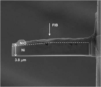
Figure 1 Lateral view of the NiO/Ni lamella. The NiO thickness (left) varies from 120 nm to 160 nm. The NiO/Ni interface is evidenced (see text for details). The direction of the STEM beam is perpendicular to the image plane, the FIB direction is shown. Reprinted with permission from Cambridge University Press, © 2013, see [Reference Armigliato11].

Figure 2 Top view of the lamella, showing the 10 μm long wedge. The local thickness at the apex of the wedge is ranging from 120 nm (top) to 320 nm (bottom). The FIB (and TEM e-beam) directions are shown. Reprinted with permission from Cambridge University Press, © 2013, see [Reference Armigliato11].
As previously reported [Reference Armigliato11], by properly choosing the milling conditions, no stoichiometry change detectable by EDS was introduced into TEM lamellas by the FIB preparation; no peak from the Ga+ ion beam was detected in the X-ray spectra.
Experimental STEM+EDS details
A 200 kV FEI Tecnai F20 FEG-(S)TEM, equipped with a high-angle annular dark-field (HAADF) detector, the TIA (Tecnai Interface Analysis) software, and an EDAX Sapphire Si(Li) detector, were employed for X-ray microanalysis of both the NiO/C sample and the NiO region of the wedge-FIBed NiO/Ni lamella. The acquisition of X-ray spectra was performed in several areas of the NiO/C sample and along 10-point linescans (3 μm long) in the case of the lamella, using in both cases an electron beam current of 1 nA in a 1 nm spot, in a stationary mode; no damage induced by this high-current density was observed. The CK, OK, and SiK integrated peak intensities were obtained by the ES Vision software (Emispec Systems Inc, www.fei.com) of the microscope.
For the MC analysis, three different specimen tilt angles toward the detector were used: 10°, 15°, and 20°, whereas the C-L analysis, based on the extrapolation technique, was performed only at a 20° specimen tilt. Because of the need for analyzing both the NiO film and the 20 nm thick amorphous carbon layer, and to minimize carbon contamination, the sample temperature was kept at 100°K during the analysis by using a Gatan LN2-cooled double-tilt holder. The anti-contamination cold finger was also used in both cases to further prevent sample contamination. To reduce sample drift during the analysis, the automatic anti-drift correction, available in the TIA software by FEI, was employed.
Results
Analysis of the NiO/C test sample by MC method
Figure 3 shows a sketch of the investigated sample in the two possible orientations with respect to the incident electron beam of the STEM: grid downward (Figure 3a) and grid upward (Figure 3b). Accordingly, the C layer is below (a) or above (b) the NiO film. Although only the former is recommended for general analysis, mounting the sample in both orientations successively was useful for our MC analysis of the bilayer. In addition, as it will be shown later on, the result of this test can be extended to the detection of a carbon contamination overlayer and to its effect on the NiO film quantification.
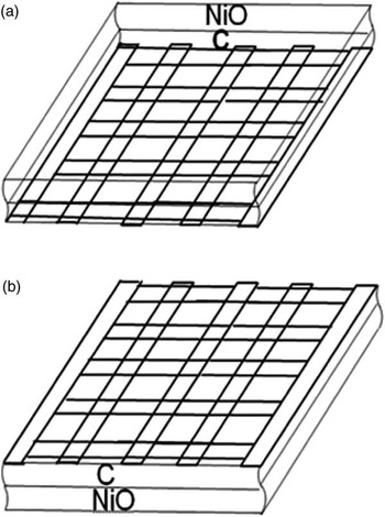
Figure 3 Sketch of the investigated NiO film, deposited on a C-coated Mo grid to show the different loading in the microscope holder. (a) grid (and C layer) below the NiO film (grid downward); (b) grid above the NiO film (grid upward). Though this latter geometry is not recommended in normal quantitative analysis, it has been analyzed by our MC method to determine the effect of a C-overlayer on the oxygen concentration in the NiO film (see text for details). Reprinted with permission from Cambridge University Press, © 2009, see [Reference Rosa and Armigliato7].
From spectra obtained in the two configurations [Reference Rosa and Armigliato7], the difference in the CK and OK peak intensity between the two geometries is clearly visible. From the net peak intensities, three ratios, I(NiK)/I(OK), I(NiK)/I(CK), and I(OK)/I(CK), were obtained. These were the experimental data inputs to our MC code.
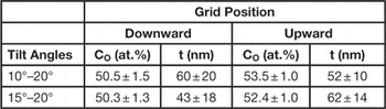
To estimate the O concentrations and the local film thickness, we employed the above-mentioned 2 tilt-angle method, previously described in [Reference Armigliato and Rosa6, Reference Rosa and Armigliato8]. We have chosen two couples of tilt angles, namely 10°–20° and 15°–20°. The former increases the differential X-ray absorption, whereas, the latter reduces the possible shadowing effect due to the specimen holder. From these results for the two geometries (Table 1), it was deduced that the oxygen concentration is in agreement with the one certified by Emitech (C(O) = 50 ± 2 at%), in the grid-downward geometry, whereas a significant deviation is obtained in the grid-upward case. This could be due to the presence of a carbon contamination on the sample surface.
Table 1 Estimates and associated errors of O concentration CO (at.%) and thickness t (nm) of the NiO film obtained by the MC 2 tilt-angle method, with the angle couples: 10°–20° and 15°–20°.
An alternative hypothesis is that the values of the physical parameters (in particular, ionization cross sections Q and detector efficiency ε) are inaccurate. But this would also affect the concentrations obtained by the 2 tilt-angle method in the grid downward geometry, which is not the case. We have also checked the absence of ice contamination in front of the detector window.
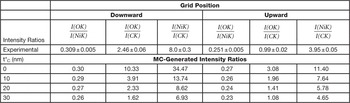
To check the hypothesis of the carbon contamination, we simulated by the 2 tilt-angle method a geometry in which, besides considering both grid positions, there is a further carbon film on the sample surface, with thickness t*C ranging from 10 nm to 30 nm. Table 2 shows that a 20–30 nm thick carbon overlayer yields similar results for both geometries, in agreement with the certified values. To further confirm this, we have used MC to obtain calculated (I(OK)/I(NiK), I(OK)/I(CK), and I(NiK)/I(CK)) intensity ratios, assuming a stoichiometric NiO composition and t*C varying from 0 nm to 30 nm. With t*C at about 20 nm, the agreement between the MC-calculated intensity ratios and the experimental intensity ratios is satisfactory in both geometries (Table 3). We point out that in Table 3 “experimental” refers to the ratios among the net integrated intensities, as obtained from the application of the ES Vision software to the experimental spectra. Obviously, a quantification can also be performed by this software (C-L method) starting from the intensities, but it is neither used in this work, nor needed for the MC calculations.
Table 2 Estimates and associated errors of O concentration CO (at.%) and thickness t (nm) of the NiO film, obtained by the MC 2 tilt-angle method, with a t*C thick carbon contaminating film on the sample surface.

Table 3 Experimental and MC-generated intensity ratios I(OK)/I(NiK), I(OK)/I(CK), and I(NiK)/I(CK). Tilt angle α = 20°.
Analysis of the NiO/Ni standard by C-L approach
Figure 4 shows a STEM image taken in the NiO region of the lamella obtained by the FIB thinning of the surface-oxidized bulk Ni standard, together with the X-ray spectra taken in 10 points along the 3 μm linescan shown as a straight line. The crosses at the end points of the linescan correspond to the position where the first and tenth spectra have been taken, which are reported in (b) and (c), respectively. The red square box was used for the antidrift correction by the cross-correlation method. The OK and the NiK peaks were used for quantification purposes. It is worth noting that no GaK peak from the Ga ion beam of the FIB is visible.
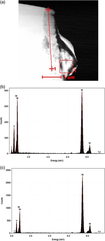
Figure 4 STEM image of the NiO/Ni lamella and EDS spectra taken on a 3000 nm long linescan. (a): the NiO film is almost vertical and clearly distinguishable from the bulk Ni substrate on its left. The two red crosses correspond to the thinnest (top) and the thickest (marked as 1) analyzed points, respectively. The square box on the right (also marked #1) is used by the software TIA of the Tecnai STEM for the drift correction with the cross-correlation method. (b) EDS spectrum taken in the thinnest point of the linescan. In addition to the OK and the NiK (and NiL) peaks, a small carbon peak is visible. (c) EDS spectrum taken in the thickest point of the linescan. Note the much higher vertical full-scale value with respect to the spectrum on the left. Tilt angle: α=20°. Reprinted with permission from Cambridge University Press, © 2013, see [Reference Armigliato11].
According to [5], the procedure to get k(O-Ni) is based on the following steps:
a) The 10 spectra are quantified with the C-L equation, assuming a stoichiometric composition and putting all k-factors equal to 1, under the thin-film approximation (no absorption).
b) A plot of C(O) and C(Ni) concentrations versus net NiK X-ray intensity is drawn.
c) The chart is fitted with a linear trendline.
d) The trendline, extrapolated to zero thickness, represents a virtual concentration.
e) Dividing the true concentration ratio by the virtual concentration ratio yields the measured k(O-Ni) factor. Namely, k(O-Ni)wt or k(O-Ni)at values will be obtained for true concentrations given in wt% or at%, respectively.
In our case, linear extrapolation of OK and NiK intensities to zero yields C(O) = 21.6 ± 0.7 and C(Ni) = 78.4 ± 0.7 (virtual concentrations, Figure 5), respectively, as:
 $$k({\rm O{\hyphen}Ni})={\textstyle{{[C({\rm O})/C({\rm Ni})]stoichiometric} \over {[C({\rm O})/C({\rm Ni})]virtual}}}$$
This results in k(O-Ni)wt = 0.99 and k(O-Ni)at = 3.63. These experimental values are quite different from the k(O-Ni)wt = 1.30 theoretical value calculated by the ES Vision software

Figure 5 Plot of O and Ni concentrations versus NiK intensity, generated in the different points in the linescan. The curves are fitted with a linear trendline. The extrapolation to zero intensity (thickness) yields virtual concentrations, where from the experimental C-L coefficient k(O-Ni) can be calculated (see text for details) [Reference Giannuzzi10].
(corresponding to k(O-Ni)at = 4.77). It must be also noted that the contribution to the primary OK intensity from the secondary fluorescence by the NiL X rays is of the order of 10-3, thus quite negligible [Reference Armigliato11]. Finally, we observe that to obtain k(O-Ni) values, this method does not require the knowledge of the detector efficiency ε (unlike MC [see previous paragraph], and the C-L method based on theoretical k factors).
Analysis of the NiO/C test sample by the C-L method
Let us now turn back to the NiO/C test sample. Having determined the experimental k value, the quantification of the NiO test sample by the C-L method can be repeated with better accuracy. The analysis was carried out by determining the OK and NiK X-ray intensities from spectra taken in this film, in both the grid-downward and grid-upward geometry, in the same experimental conditions as in the above-reported experiment on the wedge FIB lamella. The calculation of the Ni-O film composition, performed in the former geometry assuming the above-reported absorptionless k(O-Ni)at = 3.63 value and an absorption correction calculated by MC for a thickness of 55 nm, yields an oxygen concentration in agreement with the 2 tilt-angle MC method (Table 4). This result confirms the correctness of the experimental C-L factor k value obtained in this paper.
A quite different NiO composition is found by the C-L method in the grid-upward geometry. In this case the deviation from the stoichiometry is about 11 at%. This clearly indicates the inherent limitation of this analytical method, which assumes that the sample consists of a single, ternary C-O-Ni film. A still worse quantification can be expected for overlayers consisting of elements heavier than carbon.
In Table 4 the O and Ni concentrations (at.%) are summarized. They were obtained by the two methods (MC and C-L) in the two geometries.
Table 4 Comparison between the MC and C-L concentrations obtained from the NiO test sample in the two geometries.
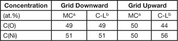
a2-tilt method, assuming t*C is about 20 nm; bwith experimental k(O-Ni)at = 3.63.
Discussion
The most accurate and reliable quantification of thin films by X-ray microanalysis in a (S)TEM can be obtained if the contribution to the experimental spectra of any carbon layer placed above and/or below a binary alloy is taken into account. This is particularly important when the sample contains light elements. To this end, application of the MC method [Reference Armigliato and Rosa6, Reference Armigliato and Rosa8] has proven to be useful because, unlike analytical approaches such as the C-L method, it can treat a specimen consisting of a stack of thin films. In fact, MC can accurately calculate the X rays generated in each layer according to the ionization cross section of the different elements at every step of the electron trajectories. The number of transmitted X rays is obtained applying the proper absorption correction. In contrast with MC, given a spectrum containing three or more peaks (CK, OK, NiK, and NiL in our case), the C-L method infers that the sample consists of a single, ternary C-O-Ni film. This leads to an inaccurate quantification of the film of interest when it is covered by one or more overlayers.
In this work we used a standard NiO sample deposited onto a grid covered with a carbon support film. From the OK and NiK intensities measured in the experimental spectra taken in the two possible sample geometries (grid downward and grid upward), MC calculation yields a NiO film composition in good agreement with the certified one only in the former case. However, if also the C-K experimental intensity is included in the MC simulations, it turns out that the a full agreement is obtained by assuming the presence of a contamination C overlayer at the sample surface (in both geometries).
As mentioned above, the C-L method could not be applied to this situation as it can treat only samples consisting of one layer. However, if the sample is mounted in the grid-downward geometry, MC shows that the influence on the NiO composition of the carbon overlayer is not significant.
It is important to experimentally determine the k(O-Ni) factors when using the C-L method. The best way, in our opinion, is to fabricate a wedge-thinned NiO/Ni standard by FIB milling. This allows one not only to obtain the factor by the extrapolation method, but also to check its correctness by calculating the Ni and O concentration in the different analyzed points; the absorption correction can be easily evaluated because the local thickness can be accurately measured on the basis of the wedge geometry.
Conclusions
The quantitative X-ray microanalysis by (S)TEM of a commercial, certified, 55 nm thick NiO film, deposited on a 20 nm carbon layer, has been performed by both the MC and the C-L methods. The presence of a few tens nm thick carbon contamination at the sample surface, revealed by MC, does not affect significantly the NiO quantification when working in proper experimental conditions. This makes the C-L method applicable, even though, unlike MC, it cannot analyze stacks of films. The required k(O-Ni) C-L factors have been experimentally determined by the extrapolation method applied to a wedge-shaped lamella, thinned by the FIB technique.


