


Introduction
Recently there has been a lot of discussion on the Microscopy Listserver about the fact that it frequently seems to take forever for a vacuum system to pump down to an operating level. It turns out that there are several interesting and fundamental reasons for this. Because of the widespread interest in this topic, it would seem worthwhile to review these reasons briefly. I think that anyone who works with an instrument that has a vacuum system could find this article useful. I am afraid, however, that the fact that it contains a number of mathematical equations will scare some people away. This should not be so, because no difficult mathematical manipulations are involved, and all the equations form the basis for interesting and important relationships, which I hope are described in straightforward, understandable terms.
Characteristics of a Vacuum
The ideal gas equation. To begin, it will be useful to review some of the relevant characteristics of a vacuum. Fundamentally, the pressure P exerted on the walls of a container of volume V by a number n moles of gas at a temperature of T Kelvins (K = °C + 273) is given by the ideal gas equation:
 $$
P = nRT/V
$$
$$
P = nRT/V
$$The preferred unit of pressure in the International System of Units is the Pascal (1 Pa = 1 Newton per square meter), and the preferred unit of volume is the cubic meter. When these units are used, the value of the gas constant R = 8.3144 Pa•m3/mole•K. The cubic meter is an inconveniently large unit of volume for most purposes, so if the liter is used instead, R = 8314.4 Pa•l/mole•K or R = 83.144 mbar•l/mole•K, where the millibar (1 mbar = 10−3 atmospheres) is another SI unit of pressure.
Older units for pressure. Originally pressures were measured with mercury manometers and were expressed in units of mm of mercury, which has since been renamed the Torr in honor of Evangelista Torricelli, the first scientist to measure the pressure of the atmosphere. Thus, 1 Torr = 133 Pa; 1 Pa = 0.0075 Torr, and R = 62.36 Torr•l/mole•K. The standard atmosphere or bar is about 760 Torr and has been defined as 100,000 Pa. Thus, 1 millibar = 100 Pa. In older vacuum work, it was also common to use two other units related to the mm Hg unit: the micron (1 μ = 10−3 Torr), which corresponds to the bottom of the rough vacuum range, and the millimicron (1 mμ = 10−6 Torr), which was once considered to be the bottom of the high vacuum range. Now the high-vacuum range is generally considered to extend to 10−7 Torr, and lower pressures are considered to be in the ultra-high vacuum range.
Concentration of gas molecules. The simple relationship almost everyone learns in elementary chemistry is that one mole of gas (1 mole = 6.023 × 10²³ molecules) occupies a volume of 22.4 liters at 0 °C (273 K) and one atmosphere pressure. Mathematically, the Kinetic Molecular Theory produced the following equation:
 $$
{\rm Number\ of\ gas\ molecules\ per\ liter} = \beta = 7.24 \times 10^{19} (P/T)
$$
$$
{\rm Number\ of\ gas\ molecules\ per\ liter} = \beta = 7.24 \times 10^{19} (P/T)
$$with pressure in Pa and temperature in Kelvins. Note that this equation does not include a dependence on the molecular mass of the gas. At ambient temperature (20°C or 293 K) the equation becomes:
 $$
\beta = 2.47 \times 10^{17} P{\rm\ molecules\ per\ liter\ for\ }P{\rm\ in\ Pa,\ or}
$$
$$
\beta = 2.47 \times 10^{17} P{\rm\ molecules\ per\ liter\ for\ }P{\rm\ in\ Pa,\ or}
$$ $$
\beta = 3.29 \times 10^{19} P{\rm\ molecules\ per\ liter\ for\ }P{\rm\ in\ Torr}
$$
$$
\beta = 3.29 \times 10^{19} P{\rm\ molecules\ per\ liter\ for\ }P{\rm\ in\ Torr}
$$These equations reveal that there are 2.5 × 10¹⁹ molecules of air in every cubic centimeter at atmospheric pressure. There are 3.3 × 10¹³ molecules per cc at the bottom of the rough vacuum range, 3.3 × 10⁹ per cc at the bottom of the high vacuum range, and at a pressure of 10−8 Pa (7.5 × 10⁻¹¹ Torr), which is well into the ultra-high vacuum range, there are still 2.5 × 10⁶ (more than two million!) molecules in each cc. The point here is that even the best vacuums we are capable of producing are still heavily populated with gas molecules!
Molecular motion. Due to their thermally activated kinetic energy, gas molecules are constantly moving in random directions at surprisingly high speeds. According to the Kinetic Molecular Theory, their speeds σ are given by the equation:
 $$
\sigma = 145.5\sqrt {(T/M)} {\rm\ meters\ per\ second}
$$
$$
\sigma = 145.5\sqrt {(T/M)} {\rm\ meters\ per\ second}
$$where M = the mass of a mole of gas. At room temperature (T = 295 K) oxygen molecules (M = 32 g/mole) fly around with speeds of about 1,000 mph, whereas lighter hydrogen molecules (M = 2 g/mole) have speeds of nearly 4,000 mph.
The important fact to be emphasized here is that vacuum pumps do not “suck,” or attract, gas molecules out of vacuum systems! What they actually do is capture a few gas molecules and remove them from a space at the end of the pumping line. This reduces the concentration of molecules in that space, whereupon molecules from neighboring regions of higher concentration instantly move in to fill the vacancy. This slight reduction in concentration rapidly propagates into the rest of the system, so when this process is repeated frequently enough and long enough, it eventually reduces the concentration of molecules in the entire system, creating a vacuum therein.
Mean free path. The average distance gas molecules travel between collisions with one another, their mean free path, is a very important characteristic because it determines how they behave when they flow through the components of vacuum systems. For air at 20°C, the mean free path λ is given with sufficient accuracy for our purposes by the following:
 $$
\lambda = 6.6/P{\rm\ mm\ for\ pressures\ in\ Pa,\ or}
$$
$$
\lambda = 6.6/P{\rm\ mm\ for\ pressures\ in\ Pa,\ or}
$$ $$
\lambda = 0.049/P{\rm\ mm\ for\ pressures\ in\ Torr}
$$
$$
\lambda = 0.049/P{\rm\ mm\ for\ pressures\ in\ Torr}
$$At atmospheric pressure and ambient temperatures, the mean free path for air molecules is only 7 × 10⁻⁸ m = 70 nm, or about 200 atom diameters. At 10−3 Torr, the bottom of the rough vacuum range, λ increases to about 50 mm (about 2 inches); at 10−4 Torr, the top of the high vacuum range, it becomes about 500 mm (nearly 20 in.); and at 10−7 Torr, the top of the ultra-high vacuum range, it becomes an incredible 500,000 mm (roughly 0.3 mile). The important thing to note here is that at all pressures below the rough vacuum range the mean free path of air molecules is larger than the internal dimensions of most components of most ordinary vacuum systems.
Flow through Circular Tubes
Viscous flow. The Knudsen number, which is the ratio of the mean free path of the gas molecules λ to the internal diameter D of the tube through which they are flowing (i.e., Kn = λ/D), is the function commonly used to characterize the flow of gas through circular tubes. This is a dimensionless quantity, and so λ and D must be measured in the same units. Then, if Kn <0.01 (λ <0.01D), gas flow is said to be viscous in character. Using equations (5a) and (5b) cited above, the condition for viscous flow can also be written as P > 5/D or D > 5/P, for P in Torr and D in mm, or P > 660/D if pressure is measured in Pa.
Under these conditions the gas molecules collide with one another more frequently than they collide with the walls of the tube through which they are flowing, and so they are swept along by the surrounding molecules producing a cooperative mass flow process. One very important consequence of this molecular interaction is that the molecules all move in the same general direction and backstreaming is impossible! That is, no molecules can move a significant distance in a direction opposite to that of the mass flow. This means that oil vapors and other contaminants cannot move from a vacuum pump into the vacuum system during periods of viscous flow.
Viscous flow will occur at pressures greater than about 65 Pa (~0.5 Torr) in tubes 10 mm in diameter and at pressures above 13 Pa (~0.1 Torr) for tubes 50 mm. Note that the maximum pressure conditions for viscous flow do not extend below 13 Pa (10−1 Torr), but that this pressure is not near the bottom of the rough vacuum range (0.133 Pa or 10−3 Torr). This can lead to problems in systems with oil-sealed rotary vane roughing pumps, because such pumps are capable of producing pressures of 1.3 Pa (10−2 Torr) or lower (see Figure 1). If such systems are evacuated for long periods of time by the roughing pump alone, the pressure in the pumping line can drop below the viscous flow range (10 Pa or 10−1 Torr).

Figure 1: A diagram depicting the basic components of vacuum systems and showing the definition of the basic evacuation parameters in terms of throughput Q.
Frictional heating and microscopic shear between the fast-moving rotor and the pump chamber can break pump oil molecules down into smaller molecular fragments that are more volatile than the oil itself. These molecular fragments can easily diffuse through the roughing line back into the system's work chamber and badly contaminate it. Leaving a system under vacuum is a good way to keep it “clean,” but not if in doing so it is continuously pumped on by an oil-sealed rotary vane pump.
Viscous conductance. The relative ease with which the components of vacuum lines accommodate the flow of gas through them is called their conductance. The conductance of circular tubes for the viscous flow of air at ambient temperature is given, with sufficient accuracy for our purposes, by the equation:
 $$
C_{cv} = 8.2 \times 10^{ - 5} (D^4 /L)P_{av} {\rm\ liters/min}
$$
$$
C_{cv} = 8.2 \times 10^{ - 5} (D^4 /L)P_{av} {\rm\ liters/min}
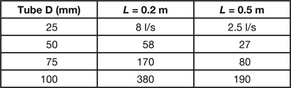
$$where D is the diameter of the tube (mm), L is its length (m), and P av is the average pressure = (P hi + P lo)/2 expressed in Pa. If P is measured in Torr, D in inches, and L in feet, the constant becomes 1.45 × 10⁴. One very important fact to note here is that viscous conductance increases as the fourth power of tube diameter; therefore, a small difference in tube diameter makes a large difference in conductance. Table 1 shows conductance values in liters per minute for tubes one meter long for two average pressures in the rough vacuum range, 1000 Pa = 7.5 Torr, and 10 Pa = 7.5 × 10⁻² Torr.
Table 1: Conductance under viscous conditions in one-meter tubes of various tube diameters.

These values are very large compared to the speeds of most roughing pumps, which range from about 50 to 200 l/min; consequently, rough pumping operations usually require very little time.
Molecular flow. At sufficiently low pressures, the mean free path of the gas molecules becomes greater than the diameter of the tubes through which they are flowing; the Knudsen number takes on a value greater than one, that is, Kn = λ/D > 1 (λ > D); and gas molecules collide more frequently with the walls of the tube than they do with one another. Under these circumstances gas flow is said to be molecular in character. Here the gas molecules move randomly, at high speeds, in all directions, and independently of each other; therefore, backstreaming is always present! Roughly,
 $$
N_b /N_p = P_p /P_s
$$
$$
N_b /N_p = P_p /P_s
$$meaning that the ratio of the number of backstreaming molecules N b to the number moving toward the pump N p is equal to the ratio of the pressure at the pump P p to that in the system work chamber P s. For example, toward the end of a pump-down process, P p might be one-tenth the pressure in the system (that is, P p = 0.1 P s), whereupon P p/P s = 0.1 and N b = 0.1 N p; that is, one-tenth as many molecules would be backstreaming as would be moving into the pump. For most systems molecular flow can be considered to occur at pressures below the rough vacuum range (below 0.13 Pa ~ 10−3 Torr).
Molecular conductance. The conductance of circular tubes for the flow of air under conditions of molecular flow at ambient temperature can be calculated, with sufficient accuracy for present purposes, using the equation:
 $$
C_{cm} = 0.0121D^3 /(100L + 0.133D){\rm\ liters/sec}
$$
$$
C_{cm} = 0.0121D^3 /(100L + 0.133D){\rm\ liters/sec}
$$where D is the tube diameter in mm, and L is its length in meters. There are three important characteristics of molecular conductance to note: (1) it does not involve a dependence on pressure, (2) it increases with the third power of the tube diameter, which is less than the fourth power dependence of viscous conductance, and (3) it decreases more rapidly with tube length than does viscous conductance. Approximate values for the molecular conductance (liters/sec) of tubes of several common diameters and 200 and 500 mm in length are shown in Table 2.
Table 2: Conductance under molecular conditions for two tube lengths and various tube diameters.
These values are generally small compared with the speeds of most pumps used in the high and ultra-high vacuum range, which typically range from 100 to 3000 liters per second.
Throughput. The quantity of gas (that is, the number of moles or molecules) flowing through a vacuum line per unit time (min or sec) is termed the throughput Q. This quantity is expressed in units of Torr·liters or Pascal·liters per minute in the rough vacuum range and per second at lower pressures. One Pa·liter is the amount of gas in one liter at a pressure of one Pa, and for T = 293 K this can be calculated using the ideal gas equation to be:
 $$
n = PV/RT = (1 \times 1)/(8314.4 \times 293) = 4.1 \times 10^{ - 7} {\rm\ moles}
$$
$$
n = PV/RT = (1 \times 1)/(8314.4 \times 293) = 4.1 \times 10^{ - 7} {\rm\ moles}
$$ $$
= 4.1 \times 10^{ - 7} \times 6.023 \times 10^{23} {\rm\ molecules/mole}
$$
$$
= 4.1 \times 10^{ - 7} \times 6.023 \times 10^{23} {\rm\ molecules/mole}
$$ $$
= 2.5 \times 10^{17} {\rm\ molecules}
$$
$$
= 2.5 \times 10^{17} {\rm\ molecules}
$$Likewise, one Torr·liter = 5.5 × 10⁻⁵ moles or 3.3 × 10¹⁹ molecules.
Then with P p being the pressure at the inlet of the pump and P c being the pressure at the outlet of the vacuum work chamber:
 $$
{\rm pumping\ speed\ is\ defined\ as\ }S_p = Q/P_p
$$
$$
{\rm pumping\ speed\ is\ defined\ as\ }S_p = Q/P_p
$$ $$
{\rm evacuation\ speed\ is\ defined\ as\ }S_e = Q/P_c
$$
$$
{\rm evacuation\ speed\ is\ defined\ as\ }S_e = Q/P_c
$$ $$
{\rm conductance\ of\ the\ pumping\ line\ as\ }C = Q/(P_c - P_p )
$$
$$
{\rm conductance\ of\ the\ pumping\ line\ as\ }C = Q/(P_c - P_p )
$$all being expressed in units of liters/min in the rough vacuum range and liters/sec at lower pressures. Then writing the reciprocal of Equation (12) yields:
 $$
1/C = (P_c /Q) - (P_p /Q) = (1/S_e ) - (1/S_p ),
$$
$$
1/C = (P_c /Q) - (P_p /Q) = (1/S_e ) - (1/S_p ),
$$which can be rearranged to give the following two important equations:
 $$
S_e = S_p C/(S_p + C)
$$
$$
S_e = S_p C/(S_p + C)
$$ $$
S_e /S_p = C/(S_p + C)
$$
$$
S_e /S_p = C/(S_p + C)
$$These equations show that the conductance of the pumping line has an overwhelming influence on the speed of evacuation.
In effect, the conductance of the pumping line can be considered as a factor degrading the efforts of the pump. For example, if the conductance is equal to the speed of the pump, the speed of evacuation will be only one half the speed of the pump. Even if the conductance is four times the speed of the pump, the speed of evacuation will be only 0.8 S p. The only way to have the speed of evacuation equal to the full speed of the pump is to install the pump directly onto the vacuum chamber!
The Evacuation Process
Rate of evacuation. The rate at which the pressure inside the vacuum chamber P c decreases with time t is called the rate of evacuation. Mathematically this is related to the speed of evacuation by the equation:
 $$
{\rm d}P_c /{\rm d}t = - (P_c /V_c )S_e
$$
$$
{\rm d}P_c /{\rm d}t = - (P_c /V_c )S_e
$$where dP c is the incremental amount P c decreases in an increment of time dt inside a chamber of volume V c, expressed in Pa or Torr per minute in the rough vacuum range and per second at lower pressures.
Ultimate pressure. Invariably, this decrease in pressure is opposed by an influx of gas q, at a rate q/V c, from several sources, principally, leaks and desorption of gas molecules from surfaces inside the vacuum system. Adding this effect, the above equation becomes:
 $$
{\rm d}P_c /{\rm d}t = (q/V_c ) - (P_c /V_c )S_e .
$$
$$
{\rm d}P_c /{\rm d}t = (q/V_c ) - (P_c /V_c )S_e .
$$As the evacuation proceeds, the pressure in the chamber will decrease. This causes the magnitude of the second term to decrease, and ultimately it will become equal to the value of the first term, whereupon the rate of evacuation becomes zero; that is, dP c/dt = 0 and q/V c = (P c/V c)S e. The pressure in the system at this point is called the ultimate pressure, P u. Substituting P u for P c in this equation yields this important relationship:
 $$
P_u = q/S_e
$$
$$
P_u = q/S_e
$$showing that the ultimate pressure attainable in a vacuum system depends as critically on the level of gas influx as on the speed of evacuation. Thus, attaining a low ultimate pressure requires a low level of gas influx (a clean, leak-free system) as well as a high speed of evacuation (short pumping lines of large diameter and high-speed pumps).
Pump-down equation. Substituting this relationship for q into Equation (16) for the rate of evacuation gives:
 $$
{\rm d}P_c /{\rm d}t = (P_u /V_c )S_e - (P_c /V_c )S_e
$$
$$
{\rm d}P_c /{\rm d}t = (P_u /V_c )S_e - (P_c /V_c )S_e
$$Separating variables, performing an integration, and solving for t yields the following equation for pump-down time:
 $$
t = (V_c S_e )\ln [(P_i - P_u )/(P_t - P_u )]
$$
$$
t = (V_c S_e )\ln [(P_i - P_u )/(P_t - P_u )]
$$Here P i is the initial pressure, P t is the pressure after pumping for a time t, and P u is the ultimate pressure for the system. Operationally, P i can be considered as the pressure at the start of a stage of the evacuation process, P t as the pressure at which the system can be put into use, whereupon t becomes the pump-down time. The term “ln” indicates the Napieran logarithm (base e = 2.71828) of the quantity that follows in square brackets.
In any practical vacuum system the ultimate pressure P u will be less than P i and P t by at least a factor of ten, and so it can be neglected, whereupon the equation simplifies to:
 $$
t = (V_c /S_e )\ln [P_i /P_t ]
$$
$$
t = (V_c /S_e )\ln [P_i /P_t ]
$$However, there is a serious shortcoming to this equation. Namely, it implies that the speed of evacuation remains constant throughout the evacuation process. Actually, both the conductance of the vacuum lines and the speed of the vacuum pumps can vary as the pressure decreases. This shortcoming can be overcome, with sufficient accuracy for most practical purposes, by dividing the pressure range into small increments, calculating the time for each increment, assuming C and S p to be constant over that increment, and adding these incremental times to obtain the total pump-down time.
Calculation of rough pumping time. For purposes of illustration, assume we have a scanning electron microscope (SEM) whose internal volume V c is about 20 liters that is rough pumped by a pump with a speed rated at 100 liters per minute through a hose that is 20 mm in diameter and 1.5 meters long (Figure 2). Then the step-wise calculation of the time for the rough pumping operation is illustrated in Table 3. Here the calculations have been carried out for pressures from atmospheric (105 Pa) down to 10 Pa in four increments (P i to P t). Conductance values were calculated for an average pressure (P av = 0.5(P i + P t)) using Equation (6). The speed of the pump was assumed to remain constant at the rated value of 100 l/min. Note that because of the overwhelmingly large values of the conductance, the speed of evacuation is essentially the same as the speed of the pump for all four stages. The time calculated for each stage is of the order of one-half minute. Thus, the total time for the rough pumping operation is calculated to be about two minutes, a value about the same as observed in practice.
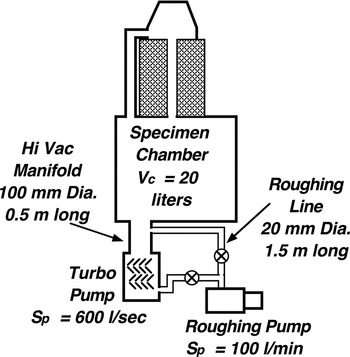
Table 3: Calculation of time for rough pumping.

Calculation of time to pump down to an operating level. Now assume that the high vacuum in our SEM is produced by a turbomolecular pump with a rated speed of 600 liters per second that is connected to the vacuum chamber by a tube 100 mm (~4″) in diameter and 0.5 meter long. Table 4 shows step-wise calculation of the time to pump down from a rough vacuum of 10 Pa (7.5 × 10⁻² Torr) to a rather low operating pressure of 10−3 Pa (7.5 × 10⁻⁶ Torr), using Equation (8) to calculate the conductance at the midrange of each interval, and with C, S p, and S e now in units of liters per second and time in seconds.
Table 4: Calculation of time to pump down to operating level.

In this pressure range, where flow is molecular in character, the conductance of the pumping line remains constant while the speed of the turbo pump and the speed of evacuation both increase as the pressure decreases. However, the total calculated pump-down time is less than one second! Anyone familiar with operating an SEM would immediately call this unrealistically short. A more realistic pump-down time would be somewhere in the range from 10 to 20 minutes, or several thousand times greater than the time just calculated. This large discrepancy is due to the fact that the influence of gas influx q, introduced in Equation (6), was subsequently neglected in the simplifying assumptions that were made in deriving Equation (20) that was used to make these calculations. The time calculated here probably corresponds closely to the time needed to remove the free gas molecules from the SEM.
Effect of gas influx. Equation (17) shows that the rate of gas influx q critically determines the ultimate pressure attainable in a vacuum system; therefore, it should be no surprise that it also plays a major role in determining the time required to pump a system down through the high vacuum range to an operating vacuum level. A simple equation for estimating this dependency is:
 $$
t \approx 3 \times 10^{ - 6} /R_t {\rm\ min}
$$
$$
t \approx 3 \times 10^{ - 6} /R_t {\rm\ min}
$$where t is the pump-down time (min) needed to reduce the rate of influx R (Pa·l/sec per mm2) due to desorption of gas molecules from surfaces inside the vacuum chamber to a level R t that is low enough to be removed by the pumping system having a throughput Q at the operating pressure. In the present example the rate of gas removal from the system at 10−3 Pa is Q = S eP c = 145 × 10−3 Pa·l/sec. It is extremely difficult to know the total internal surface area that is effective in desorbing gas molecules because this quantity is strongly dependent on such factors as surface roughness and surface preparation. However, 5 × 105 mm2 might be a reasonable value to assume for present purposes. Then the rate of gas desorption at the operating pressure would need to be less than R t = 145 × 10−3/ 5 × 105 = 2.9 × 10⁻⁷ Pa·l/sec per mm2. Using Equation (21) then gives:
 $$
t \approx 3 \times 10^{ - 6} /R_t \approx 3 \times 10^{ - 6} /2.9 \times 10^{ - 7}
$$
$$
t \approx 3 \times 10^{ - 6} /R_t \approx 3 \times 10^{ - 6} /2.9 \times 10^{ - 7}
$$ $$
\approx 10{\rm\ minutes\ for\ the\ pump-down\ time}{\rm .}
$$
$$
\approx 10{\rm\ minutes\ for\ the\ pump-down\ time}{\rm .}
$$This is a more reasonable value than that calculated in Table 4 and is in the general range of pump-down times experienced in practice. Although several rough estimates were involved in reaching this result, it nonetheless illustrates the fact that gas influx is an overriding factor in determining the time required to pump a vacuum system down to an operating level below the rough vacuum range.
Water vapor is the gas most heavily involved in this gas desorption process. Water molecules are highly polar in character and therefore adsorb strongly and desorb most reluctantly from surfaces inside a vacuum system. The atmosphere normally contains several percent water vapor, and so there is an abundance of water molecules available to adsorb onto the internal surfaces of a vacuum system every time it is exposed to the atmosphere. This adsorption process can, of course, be minimized by admitting a dry gas, such as dry nitrogen, rather than air, whenever it is necessary to bring the system up to atmospheric pressure. A liquid nitrogen trap in the high vacuum manifold, or a liquid nitrogen cooled cold finger in the vacuum chamber, will act as a very effective pump for water molecules and will usually speed up the pump-down process noticeably. Heating the system will also speed up the desorption process. In fact, systems designed to reach pressures in the ultra-high vacuum range are constructed so that they can be baked out for several hours at temperatures as high as 400°C. Leaks, gas evolution from such materials as silver and carbon paints, virtual leaks from such sources as gas confined in screw threads, can also contribute to the rate of gas influx and should be minimized.
Conclusions
Having to wait a long time for a vacuum instrument to pump down to an operating vacuum level is an annoying and frustrating experience. In this article an attempt has been made to explain the basic characteristics of the pump-down process and to show how they contribute to this problem. The first major factor is the construction of the pumping system, which should consist of high-speed pumps and short manifold tubes of large diameter. Unfortunately, once an instrument has been purchased there is little the ordinary user can do to change its construction. The second major factor is the influx of gas molecules inside the vacuum system, and here good maintenance procedures can have a significant effect.
I hope that this brief discussion has helped readers of Microscopy Today, who I hope also include many of those who correspond over the Microscopy Listserver, to understand the nature of this phenomenon more fully. If not, this topic is discussed in much greater detail in my book on vacuum methods [Reference Bigelow1].


