

The forecasts for the world and the UK economy reported in this Review are produced using the National Institute's global econometric model, NiGEM. NiGEM has been in use at NIESR for forecasting and policy analysis since 1987, and is also used by a group of more than 40 model subscribers, mainly in the policy community. Most countries in the OECD are modelled separately,Footnote 1 and there are also separate models for China, India, Russia, Brazil, Hong Kong, Taiwan, Indonesia, Singapore, Vietnam, South Africa, Latvia, Lithuania, Romania and Bulgaria. The rest of the world is modelled through regional blocks so that the model is global in scope. All models contain the determinants of domestic demand, export and import volumes, prices, external current account balances and net external assets. Output is tied down in the long run by factor inputs and technical progress interacting through production functions, but is driven by demand in the short to medium term. Economies are linked through trade, competitiveness and financial markets and are fully simultaneous. Further details on NiGEM are available on http://nimodel.niesr.ac.uk/.
The key interest rate and exchange rate assumptions underlying our current forecast are shown in tables A1–A2. Our short-term interest rate assumptions are generally based on current financial market expectations, as implied by the rates of return on treasury bills and government bonds of different maturities. Long-term interest rate assumptions are consistent with forward estimates of short-term interest rates, allowing for a country-specific term premium. Where term premia do exist, we assume they gradually diminish over time, such that long-term interest rates in the long run are simply the forward convolution of short-term interest rates.


The Reserve Bank of Australia and the Reserve Bank of New Zealand lowered their benchmark interest in 2016 and have since kept them unchanged. The Reserve Bank of Australia cut its rate by 50 basis points in two steps and the Reserve Bank of New Zealand reduced its rate by 75 basis points in three rounds. The People's Bank of China and the Reserve Bank of India reduced their interest rates in 2015 by a total of 125 basis points each. While the People's Bank of China has since left its benchmark rates unchanged, the Indian central bank lowered its benchmark rate further by 50 basis points in two rounds in 2016. After reducing its policy rate by 100 basis points in four steps between August 2014 and June 2015, the Bank of Korea cut it again by 25 basis points in June 2016. Indonesia's central bank reduced its benchmark interest rate by 25 basis points in February 2015, for the first time since 2012, and then lowered it again by 100 basis points in 2016 in four steps. However, after introducing a new policy rate, the 7-day reverse repurchase rate, in August 2016, its interest rates were lowered in two further steps, by 25 basis points in each case. In 2014 and 2015, the Romanian Central Bank reduced its benchmark interest rate by a total of 225 basis points in nine steps and has kept it unchanged since. The National Bank of Hungary brought its policy rate down by 120 basis points in eight rounds between the beginning of 2015 and May 2016 and has held it at 0.9 per cent since. The central banks of Norway and Poland lowered their policy rates by 50 basis points each in 2015, to 0.75 and 1.5 per cent respectively. The central bank of Norway cut its benchmark rate by a further 25 basis points in March 2016, while the central bank of Poland has left its rates unchanged. Over the course of 2015, the Swedish Riksbank cut its policy rate by 35 basis points in three rounds and lowered it again, by 15 basis points, at the beginning of 2016. At the time of writing, the Riksbank's policy rate stands at −0.5 per cent. At the turn of 2015 the Swiss National Bank cut its benchmark rate by 25 basis points to −0.75 per cent, while the Central Bank of Denmark reduced its rates by 15 basis points to just 0.05 per cent. Both central banks have left their main policy rate unchanged since then. After reducing its benchmark interest rate by a cumulative 700 basis points, to 10 per cent, in seven stages during 2015 and 2016, the Central Bank of Russia lowered it again by a total of 75 basis points in two stages in March–April 2017. The Bank of Canada has kept its benchmark interest rate unchanged, at 0.5 per cent, after lowering it by 50 basis points over two rounds in 2015. These were the Bank of Canada's first cuts in interest rates since April 2009. Following the easing of inflationary pressures and the election of a new government, the Central Bank of Brazil cut its interest rate by 25 basis points twice in the last three months of 2016 – the first time since 2012 – and lowered it by a further 250 basis points, in three steps, in January–April 2017.
In contrast, after a spell of reductions in interest rates by the Central Bank of Turkey in 2014 and 2015, inflationary pressures led to an increase in the benchmark rate by 50 basis points in November 2016. The South African Reserve Bank increased its benchmark rate– for the first time since 2008 – by 50 basis points in two rounds in 2015 and then raised it further by a further 75 basis points in two stages last year. Increases in the target range for the federal funds rate by the US Federal Reserve since December 2015, and also concerns about the trade policies of the US administration that came into office in January 2017, placed downward pressure on the Mexican peso. In order to stem this pressure, the central bank of Mexico increased its policy rate by 350 basis points in eight rounds between December 2015 and March 2017. These were the first increases since August 2008.
In March 2017, the Federal Reserve raised its target range for the federal funds rate by 25 basis points to 0.75–1.0 per cent – the third increase from the low of 0.0–0.25 per cent that applied for the seven years up to December 2015. Its median projections for the rate at the end of this year and 2018 were left unchanged, which implies that two further increases of 25 basis points are expected this year, followed by another three next year. With inflation now close to the Fed's medium-term objective, the FOMC stated that it would “carefully monitor actual and expected inflation developments relative to its symmetric inflation goal”.
The expectation of the first rate change by the Monetary Policy Committee (MPC) of the Bank of England is based on our view of how the economy will evolve over the next few years. As discussed in the UK chapter of this Review, we expect the UK economy to experience a slowdown as a consequence of the vote to leave the EU.Footnote 3 At its August 2016 meeting, to mitigate the expected downturn, the MPC introduced additional monetary stimulus, which included a reduction in Bank Rate by 25 basis points to 0.25 per cent, the purchase of £60 billion of government bonds and a programme of £10 billion of purchases of sterling-denominated non-financial corporate bonds. At the time of writing, financial markets expect the MPC to raise rates to 50 basis points by the spring of 2020, and to 70 basis points in the middle of 2021. Our view foresees an earlier rise in interest rates. We expect a 25 basis point rise in the third quarter of 2019, following the UK's two-year negotiated withdrawal from the EU. Bank Rate is expected to reach 2 per cent in the second half of 2022, with this being the point at which the MPC is assumed to stop re-investing the proceeds from maturing gilts it currently holds, allowing the Bank of England's balance sheet to shrink ‘naturally’.
The European Central Bank (ECB), at its March meeting, left its interest rates and asset purchase programme unchanged but amended its forward guidance to signify that the risk of deflation had disappeared, along with the associated sense of urgency. The Bank of Japan has left its policy parameters unchanged since September 2016.
The central banks of the Euro Area (ECB) and Japan (BoJ) continue to expand their balance sheets. The ‘expanded asset purchase programme’ of the ECB, which began in March 2015, envisaged combined purchases of assets amounting to €60 billion a month until at least September 2016. In April 2016, monthly purchases were increased to €80 billion and were expected to “run until end-March 2017, or beyond, if necessary, and in any case until the Governing Council sees a sustained adjustment in the path of inflation consistent with its inflation aim”. With inflation remaining well below the ECB's objective of ‘below, but close to, 2 per cent’, in December 2016, the ECB announced that its asset purchase programme would be extended to at least December 2017, but that starting in April purchases would revert to amounts of €60 billion per month. The ECB, at its March meeting, left its interest rates and asset purchase programme unchanged but amended its forward guidance to signify that the risk of deflation had disappeared, along with the associated sense of urgency.
In October 2014, the BoJ announced that it would expand its asset purchase programme by about 30 per cent. The expanded programme envisaged the addition of about ¥80 trillion to the monetary base annually, up from the existing ¥60–70 trillion. First in December 2015 and again in September 2016, the BoJ announced further modifications to its programme of quantitative and qualitative easing (QQE). The latest round of changes was motivated by the Bank's concern that negative interest rates, together with its asset purchase programme, via a flattening in the yield curve, posed risks to financial stability via their implications for bank profitability and pension funds' viability. Therefore the BoJ supplemented the QQE framework by ‘yield curve control’: the Bank would regulate its asset purchases to target the 10-year government bond yield, initially at zero, so that it would control long-term as well as short-term interest rates.
Figure A1 illustrates the recent movement in, and our projections for, 10-year government bond yields in the US, Euro Area, the UK and Japan. Convergence in Euro Area bond yields towards those in the US, observed since the start of 2013, reversed at the beginning of 2014. In February 2014, the margin between Euro Area and US bond yields started to widen, reaching a maximum of about 176 basis points at the end of December 2016, before somewhat narrowing to 120 basis points towards the second half of April 2017. In the second half of 2014 a wedge opened between the US and UK government bond yields, which fluctuated between 20 and 30 basis points in 2015. From the beginning of 2016, the margin started to widen, and remained within the range of about 100–140 basis points since December 2016. Looking at the levels of 10-year sovereign bond yields in the latter part of April 2017, these have decreased since the end of January in the US, the Euro Area, and the UK – by about 10–40 basis points – but remained largely unchanged in Japan. Expectations for bond yields for the end of 2017, compared with expectations formed just three months ago, are lower for the US, UK, and Japan, and largely unchanged for the Euro Area. While for the US and Japan they went down by about 10–20 basis points, for the UK, expectations for bond yields decreased by about 40 basis points.
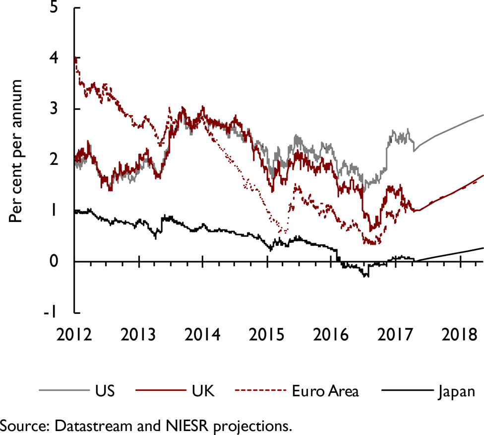
Figure A1. 10–year government bond yields
Sovereign risks in the Euro Area have been a major macroeconomic issue for the global economy and financial markets in recent years. Figure A2 depicts the spreads relative to Germany of 10-year government bond yields of Spain, Italy, Portugal, Ireland and Greece. The final agreement on Private Sector Involvement in the Greek government debt restructuring in February 2012 and the potential for Outright Monetary Transactions (OMT) announced by the ECB in August 2012 brought some relief to bond yields in these vulnerable economies. Sovereign spreads have remained stable, in most cases, since late July 2014, the most notable exception being a marked widening of Greek spreads reflecting initial uncertainty over the fiscal stance and probability of debt repayment following the formation of a government dominated by a political party elected on an ‘anti-austerity’ manifesto in January 2015. The risk of Greece leaving the Euro Area then returned to the fore, as a deal on a third bailout for Greece appeared unlikely. In the summer of 2015 a lack of liquidity led to a three-week closure of the domestic banking system, with withdrawal limits imposed upon on Greeks' bank accounts and the imposition of controls on external payments. The dangers relating to the financial difficulties of Greece and the policy programme being negotiated with its European partners subsequently receded. In mid-August 2015, it was confirmed that negotiators had reached agreement in principle on a 3-year fiscal and structural reform programme to be supported by €86 billion of financing from the European Stability Mechanism (ESM). Disbursements (including cash and cashless) totalling €31.7 billion were made by the ESM between August 2015 and October 2016. However, sovereign spreads remain elevated due to issues around long-term debt sustainability.
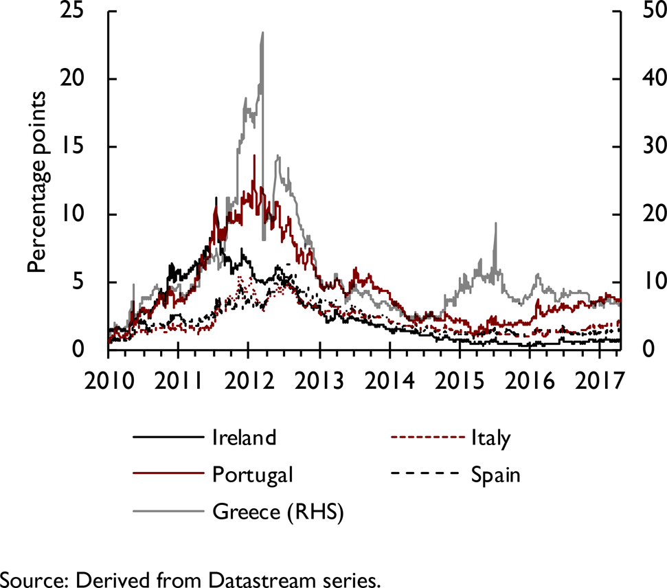
Figure A2. Spreads over 10–year German government bond yields
In Portugal sovereign spreads started to widen at the end of 2015, and throughout 2016 were around the levels last seen at the beginning of 2014. A combination of factors, including the initial ‘anti-austerity’ stance of the new Socialist government, the unexpected decision by the Portuguese central bank to impose losses on bank bonds held by international investors, the risk of a credit-rating downgrade that could result in the exclusion of government bonds from the ECB's asset-buying programme and weakness in the banking system combined with a high level of government debt (around 130 per cent of GDP) led to Portuguese bonds being the worst performers in the Euro Area after Greece.
In our forecast, we have assumed spreads over German bond yields continue to narrow in all Euro Area countries.
Figure A3 shows the spreads of corporate bond yields over government bond yields in the US, UK and Euro Area. This acts as a proxy for the margin between private sector and ‘risk-free’ borrowing costs. Private sector borrowing costs rose more or less in line with the rise in government bond yields from the second half of 2013 to the second half of 2015, illustrated by the stability of these spreads in the US, Euro Area and the UK. Reflecting the tightening of financial conditions, corporate bond spreads widened at the beginning of 2016, but subsequently have narrowed somewhat barring the jump observed around the period of the UK's decision to leave the EU. Since summer 2016 corporate bond spreads have been relatively stable in the UK, but have been on a declining trend in the US and the EA, where private sector borrowing costs have risen less than the observed rise in risk-free rates. This trend largely continued this year as well; however, by the time of writing there was marginal increase in corporate bond spreads in the US as private sector borrowing costs rose more compared to increase in risk-free rates. Our forecast assumption for corporate spreads is that they gradually converge towards their long-term equilibrium level.
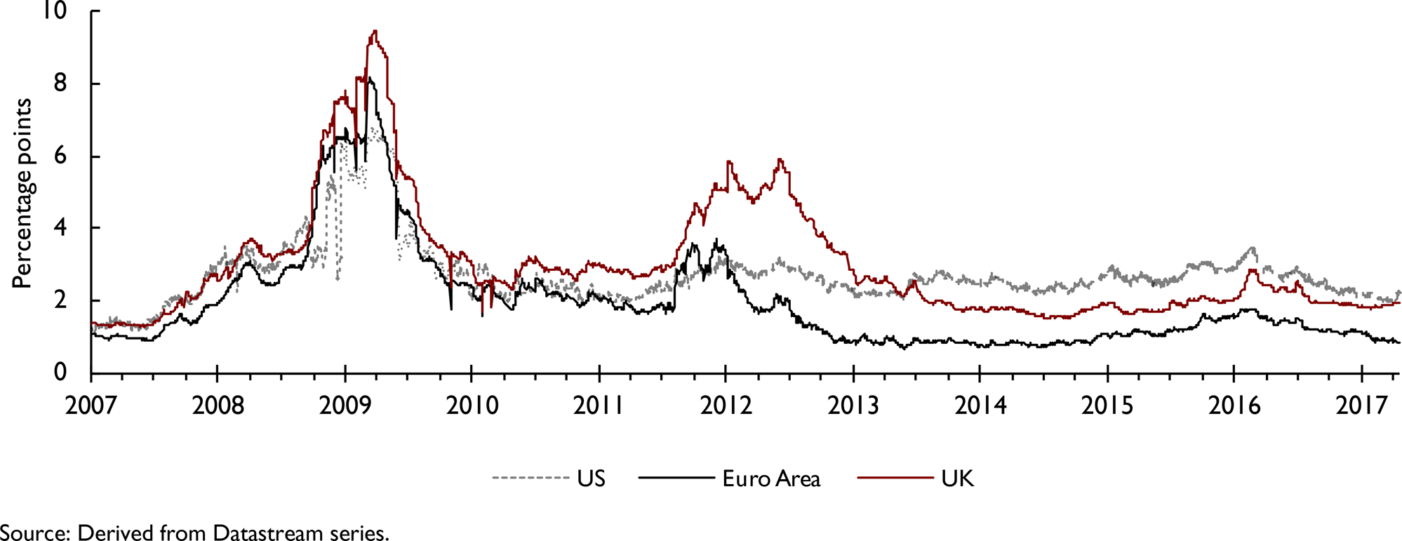
Figure A3. Corporate bond spreads. Spread between BAA corporate and 10–year government bond yields
Nominal exchange rates against the US dollar are generally assumed to remain constant at the rate prevailing on 19 April 2017 until the end of December 2017. After that, they follow a backward-looking uncovered-interest parity condition, based on interest rate differentials relative to the US. Figure A4 plots the recent history as well as our forecast of the effective exchange rate indices for Brazil, Canada, the Euro Area, Japan, UK, Russia and the US. Exchange rate movements in the period since late January 2017 have been mixed, with the US dollar broadly strengthening up to mid-March and subsequently falling back. The trade-weighted value of the US dollar in late April was little changed from late January and about 4 per cent below the 14-year peak reached at the end of last year. Since the fourth quarter of last year, in effective terms, the euro has lost about 1 per cent of its value, while the yen gained about 1 per cent. Over the same period, among the emerging market currencies, the largest movements in trade-weighted terms were a depreciation of the Turkish lira – by about 10 per cent – and appreciation of the Russian rouble and Mexican peso by about 12 and 7 per cent respectively. The Russian rouble continued to appreciate against the US dollar mainly reflecting oil price developments, while receding expectations of US action against Mexican exports and tightening of Mexican monetary policy led to the strengthening of Mexican currency.

Figure A4. Effective exchange rates
Our oil price assumptions for the short term are based on those of the US Energy Information Administration (EIA), published in April 2017, and updated with daily spot price data available up to 19 April 2017. The EIA use information from forward markets as well as an evaluation of supply conditions, and these are illustrated in figure A5. Oil prices fluctuated within a narrow range over the past three months, but in late April remained broadly unchanged from early March. Projections from the EIA suggest an increase in prices of about 10 per cent by the end of 2018 – largely unchanged from expectations three months ago. This would still leave oil prices about $48 lower than their nominal level in mid-2014. Oil prices are expected to be about $55 and $60 a barrel by the end of 2017 and 2018, respectively.
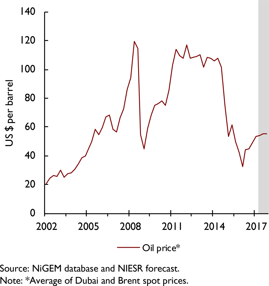
Figure A5. Oil prices
Our equity price assumptions for the US reflect the expected return on capital. Other equity markets are assumed to move in line with the US market, but are adjusted for different exchange rate movements and shifts in country-specific equity risk premia. Figure A6 illustrates the key equity price assumptions underlying our current forecast. Movements in equity markets since late January have been mixed and generally moderate. Major indices in the US reached historic highs at the beginning of March, subsequently fluctuating around slightly lower levels. In the Euro Area, since the fourth quarter of last year, equity prices in the major economies increased by between 7–18 per cent, with Italy being the best performer followed by Spain.
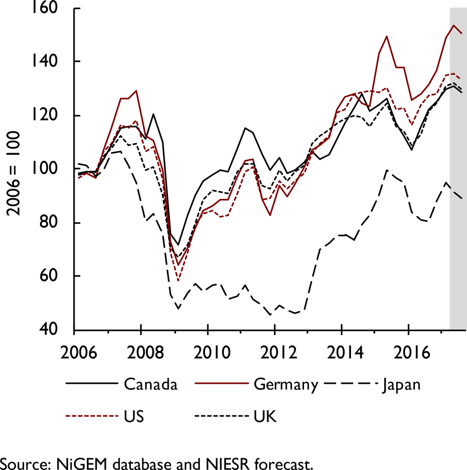
Figure A6. Share prices
Fiscal policy assumptions for 2017 follow announced policies as of 19 April 2016. Average personal sector tax rates and effective corporate tax rate assumptions underlying the projections are reported in table A3, while table A4 lists assumptions for government spending. Government spending is expected to continue to decline as a share of GDP between 2017 and 2016 in the majority of Euro Area countries reported in the table. Pressure continues to mount for a loosening of fiscal policy to support demand and indeed the decision by the European Commission in July 2016 not to recommend that fines should be levied on Portugal and Spain for not taking effective action to reduce their deficits is a sign of an easing of the discipline involved in the Stability and Growth Pact. The European Commission argued in November 2016 that, “In light of the slow recovery and risks in the macroeconomic environment, there is a case for a moderately expansionary fiscal stance for the euro area”, more specifically a fiscal expansion of up to 0.5 per cent of GDP at the level of the Euro Area as a whole for 2017. However in December 2016, the Eurogroup of Euro Area finance ministers rejected the Commission's recommendation, approving instead a neutral fiscal stance for the Area this year. A policy loosening relative to our current assumptions poses an upside risk to the short-term outlook in Europe. For a discussion of fiscal multipliers and the impact of fiscal policy on the macroeconomy based on NiGEM simulations, see Reference Barrell, Holland and HurstBarrell et al. (2012).


