


1. Introduction
In an era of social media and connectivity, the size of data has been growing exponentially as web users are becoming increasingly enthusiastic about interacting, sharing, and working together through online collaborative media (Cambria Reference Cambria2017). One way to leverage this information is opinion mining (also known as sentiment analysis), as understanding people’s opinion has a great value for both business and society.
Sentiment analysis consists of automatically extracting opinions (polarities such as positive, neutral and negative) expressed in natural languages; for instance, one should extract positive from the sentence: “I’m in love with this place!”. However, as opinion expressed by words is highly context-dependent (e.g., “This camera has a long battery life.” vs “This camera takes long to focus.”), and opposite polarities can be expressed in the same sentence (e.g., “The food is great but the service is awful .”), there is thus the need to perform sentiment analysis at a more fine-grained level: aspect level.
Sentiment analysis at aspect level, also known as aspect-based sentiment analysis (ABSA), consists of extracting the opinion associated with a predefined aspect in a sentence. For instance, consider the earlier example: “The food is great but the service is awful, ” ABSA will extract positive for the aspect food and negative for the aspect service. Usually, ABSA can be broken down into two tasks: aspect extraction and sentiment classification. In this paper, we only focus on the classification part, assuming the aspects have been extracted.
Similar to other NLP tasks, ABSA leverages deep learning to achieve state of the art performance. However, as an end-to-end approach, Deep Neural Networks (DNNs) are considered to be less flexible and robust as it is not easy to fix the model after training. For instance, later in this paper, we will see examples of a DNN model that always predicts positive when seeing obvious negative words (e.g., “terrible,” “disappointed”). To fix similar issues in an end-to-end model, it is very difficult to locate where the problem is. Of course, one could always retrain the model with additional training examples. However, in practice, new resources are not always available.
In this paper, focusing on the classification task of ABSA, we start searching for an efficient way to bridge DNN and existing language resources (sentiment lexicons) for a more robust and adaptive model architecture. Along the way, we find that the commonly used attention mechanism is likely to over-fit and force the network to “focus” too much on a particular part of a sentence, while ignoring key positions for judging the polarity. Moreover, we also explore the possibility of further improving the lexicon-enhanced neural system through domain-specific sentiment induction. In general, this paper can be divided into three main topics: lexicon enhancement, attention regularization, and sentiment induction.
1.1 Lexicon enhancement
To improve the robustness of a DNN based approach, it is natural to think of using sentiment lexicons. First, as freely available language resources, they require no extra efforts for feature engineering; second, by having a secondary input, the model should learn to leverage the information provided by the lexicon; compared to pure end-to-end approaches, a lexicon is easier to be maintained: for instance, the polarities of opinion words can be added, removed, or updated accordingly, so that the model becomes overall more robust.
In this paper, we start by replicating the AT-LSTM model (Wang et al. Reference Wang, Huang, Zhao and Zhu2016) as our baseline system on the SemEval 2014 Task 4, restaurant domain dataset. Later, we design and experiment different approaches to effectively merge sentiment lexicons with the baseline model. One of the approaches, which we name ATLX, yields notable improvement, while requiring less complexity in terms of model architecture and feature engineering. We later validate the same approach on the SemEval 2015 Task 12, laptop domain dataset. And a similar performance improvement is observed compared to the baseline. Details of the lexicon enhancement topic will be discussed in Section 3.1 for methodology and in Section 4.1 for experiments and discussion.
Note that some experiments of the ATLX model on the SemEval 2014 Task 4 data (restaurant domain) have been published in Bao et al. (Reference Bao, Lambert and Badia2019). In this paper, we report additional experiments on the SemEval 2015 Task 12 dataset (laptop domain) that support the effectiveness of the approach and additional performance tests of the ATLX model. We also include experiment results of other ATLX variants for comparison.
1.2 Attention regularization
In ABSA, the model is expected to extract opinion from the same input sentence according to different given aspects so that it makes perfect sense to allow the model to look at the input sequence differently given different aspects and be able to “highlight” relevant parts when predicting. However, we believe it is possible that the commonly used attention mechanism could over-fit by being too sparse, and this extreme sparsity in the attention vector could hurt the model by “over focusing” in particular parts of the sentence and thus “blinding” the model on key positions for polarity judgment. In recent studies, Niculae and Blondel (Reference Niculae and Blondel2017); Zhang et al. (Reference Zhang, Zhao, Li and Zong2019) proposed approaches to incentivize the sparsity in the attention vector; however, this would only encourage the over-fitting effect in such scenarios, especially when attention is applied early in the model.
In this paper, we explore the effect of regularizing attention vectors by introducing an attention regularization term in the loss function to allow the network to have a broader “focus” on different parts of the sentence. We design and experiment with two regularizers: a standard deviation regularizer and a negative entropy regularizer. Experimental results suggest that both regularizers are able to improve the baseline, where the negative entropy regularizer yields the largest improvement. Details of the attention regularization topic will be discussed in Section 3.2 for methodology and in Section 4.2 for experiments and discussion.
Note that some experiments of the attention regularizers on the SemEval 2014 Task 4 data (restaurant domain) have been published in Bao et al. (Reference Bao, Lambert and Badia2019). In this paper, we report additional experiments on the SemEval 2015 Task 12 dataset (laptop domain) that support a similar conclusion of the previous one.
1.3 Sentiment induction
Although sentiment lexicons can directly provide polarity information of opinion words to the model, it is true that the polarity of an opinion word is both domain- and context-dependent. For example, under a general context, “fallout” and “excel” carry negative and positive sentiments, respectively; but in the electronics or the laptop review domain, “fallout” or “excel” are both neutral proper nouns referring to a video game and a software. Additionally, in some cases, the same word may carry opposite sentiments in the same domain under different contexts, and this is common in ABSA: for instance, “cheap” is positive when describing the aspect price but it is definitely negative when describing the aspect quality. Thus, it is necessary to not only enable models to leverage sentiment lexicons but also adapt lexicons according to different domains and aspects.
In this paper, we are interested to see whether it is possible to further improve the ATLX system with a more fine-grained lexicon. To do that, we adopt one of the state of the art sentiment domain adaptation methods, the one by Mudinas et al. (2018), which consists of a word vector-based semi-supervised approach, and apply it to convert the general lexicon constructed for ATLX to a domain-specific one of electronics reviews. We then compare the performance gain of the general lexicon, the domain-specific lexicon, and a gold lexicon for laptop reviews labeled by ourselves by applying them in the ATLX system on the SemEval 2015 Task 12, laptop domain dataset.
As a result, we find that in general, domain-specific lexicons do improve the model performance compared to a generic one; however, the performance ceiling suggested by the gold lexicon is rather low. Moreover, as most domain adaptation works are done by recreating an existing domain-specific lexicon and neutral words are often ignored, we find that the role of neutral words is rather important when applying the adapted lexicon in the model. In addition, we also intend to create a fine-grained aspect-specific sentiment lexicon with a similar approach. However, no performance improvement could be achieved. Details regarding the sentiment induction topic will be discussed in Section 3.3 for methodology and in Section 4.3 for experiments and discussion.
2. Related work
Sentiment analysis as a valuable NLP field has been extensively studied in the past decades. Early researches of sentiment analysis date back to the beginning of the 21st century, when researchers began to realize the value of this field (Wiebe Reference Wiebe2000; Turney Reference Turney2002; Pang et al. Reference Pang, Lee and Vaithyanathan2002). In the last decades, computation power and digital data have been increasing exponentially, which enables DNN to be back under the spotlight as they yield significant improvements across a variety of tasks compared to previous state of the art methods (Barnes Reference Barnes2019; Wen et al. Reference Wen, Zhang, Zhang, Yin and Ma2020; Liu et al. Reference Liu, Zheng, Zheng and Chen2020). On the other hand, detecting and filtering neutrality (Valdivia et al. Reference Xue and Li2018) and sentiment sensing with ambivalence handling (Wang et al. 2020) have become trending. More recently, new approaches such as emotional recurrent units (Li et al. 2020), graph convolutional networks (Veyseh et al. Reference Li, Shao, Ji and Cambria2020), and multiplicative attention mechanism (Kumar et al. 2021) have become popular.
In terms of ABSA, Wei and Gulla (Reference Wei and Gulla2010) proposed a hierarchical classification model using a sentiment ontology tree that leverages the knowledge of hierarchical relationships of product attributes to better capture sentiment aspect relations. Tang et al. (Reference Tang, Qin, Feng and Liu2016) proposed Target Dependent LSTM (TD-LSTM) and Target Connection LSTM (TC-LSTM) to extend LSTM by taking the target into consideration. Ruder et al. (Reference Ruder, Ghaffari and Breslin2016) modeled the inter-dependencies of sentences in a review with a hierarchical bidirectional LSTM for ABSA, where the model is capable of leveraging both intra- and inter-sentence relations. Wang et al. (Reference Wang, Huang, Zhao and Zhu2016) proposed an attention-based LSTM with aspect embeddings, which was proven to be an effective way to enforce the neural model to attend to the related part of a sentence given different aspects. Tang et al. (Reference Tang, Qin, Feng and Liu2016) introduced a deep memory network for aspect level sentiment classification that explicitly captures the importance of each context word when inferring the sentiment polarity of an aspect. Cheng et al. (Reference Ma, Li, Zhang and Wang2017) proposed a HiErarchical ATtention (HEAT) network for ABSA, which contains a hierarchical attention module, consisting of aspect attention and sentiment attention. Ma et al. (2017) proposed Interactive Attention Networks (IAN) to interactively learn attention in the contexts and targets and generate the representations for targets and contexts separately. Liu et al. (2018) proposed a content attention-based ABSA model, which consists of two attention enhancing mechanisms: a sentence-level content attention mechanism and a context attention mechanism. Xu et al. (2019) extended ABSA to Review Reading Comprehension (RRC) that aims to turn customer reviews into a large source of knowledge that can be exploited to answer user questions, where BERT was used for post-training. Karimi et al. (2020) applied adversarial training to produce artificial examples that act as a regularization method for the BERT model on the tasks of both aspect extraction and aspect sentiment classification. Li et al. (Reference Kumar, Ashok, T. and Cambria2021) combined convolutional network and graph network and proposed a dual graph convolutional networks model to take into account syntactic relations between aspects and opinion words.
Over the years, a lot of work has been done focusing on leveraging existing sentiment lexicons to enhance the performance of deep learning based sentiment analysis systems; however, most works are performed at document and sentence level. Teng et al. (2016) proposed a weighted sum model which consists of representing the final prediction as a weighted sum of network prediction and polarities provided by the lexicon. Shin et al. (2017) used two convolutional neural networks to separately process sentence and lexicon inputs, and the final representation is then combined with an attention mechanism for prediction. Lei et al. (2018) described a multi-head attention network where the attention weights are jointly learned with lexicon inputs for classification. Barnes (Reference Barnes2019) explored the use of multi-task learning (MTL) for incorporating external knowledge in neural models by using MLT to enable a BiLSTM sentiment classifier to incorporate information from sentiment lexicons. Ren et al. (Reference Li, Sun, Han and Li2020) proposed a lexicon-enhanced attention network (LEAN) based on bidirectional LSTM. Li et al. (2020) experimented a lexicon integrated two-channel CNN–LSTM model, combining CNN and LSTM/BiLSTM branches in a parallel manner.
Regarding the attention mechanism, it is less stressed that it is likely to over-fit and force the network to ”focus” too much on a particular part of a sentence, while in some cases ignoring positions which provide key information for judging the polarity. In recent studies, both Niculae and Blondel (Reference Niculae and Blondel2017) and Zhang et al. (Reference Zhang, Zhao, Li and Zong2019) proposed approaches to make the attention vector more sparse; however, this would only encourage the over-fitting effect in such scenarios. In Niculae and Blondel (Reference Niculae and Blondel2017), instead of using softmax or sparesmax, fusemax was proposed as a regularized attention framework to learn the attention weights. In Zhang et al. (Reference Zhang, Zhao, Li and Zong2019), $L_{max}$
and Entropy were introduced as regularization terms to be jointly optimized within the loss function. Both approaches share the same idea of shaping the attention weights to be sharper and more sparse so that the advantage of the attention mechanism is maximized. However, according to our experiments, it is possible that when applied early in the network, the overly sparse attention vector could hurt the model by not passing key information to deeper layers.
$L_{max}$
and Entropy were introduced as regularization terms to be jointly optimized within the loss function. Both approaches share the same idea of shaping the attention weights to be sharper and more sparse so that the advantage of the attention mechanism is maximized. However, according to our experiments, it is possible that when applied early in the network, the overly sparse attention vector could hurt the model by not passing key information to deeper layers.
In Liu (Reference Aue and Gamon2012), it has been shown that sentiment analysis is highly sensitive to the domain from which the training data are extracted. A classifier trained using opinion documents from one domain often performs poorly on test data from another domain. The reason is that words and even language constructs used in different domains for expressing opinions can be quite different. Existing domain adaptation approaches either adapts the model or adapts a sentiment lexicon from a source domain to a target domain (Aue and Gamon Reference Tan, Wu, Tang and Cheng2005; Tan et al. Reference Pan, Ni, Sun, Yang and Chen2007; Pan et al. Reference Wu and Huang2010; Wu and Huang Reference Barnes, Klinger and imWalde2016; Barnes et al. Reference Barnes2016; Rietzler et al. Reference Kanayama and Nasukawa2020). On the other hand, a lot of research has focused on adapting generic lexicons to domain-specific ones (Kanayama and Nasukawa 2006; Wu and Wen 2010; Lu et al. Reference Bollegala, Weir and Carroll2011; Bollegala et al. Reference Mikolov, Chen, Corrado and Dean2011).
More recently, as deep learning thrives in most NLP fields, the focus of sentiment domain adaptation also shifts more to vector-based (Mikolov et al. Reference Madsen, Meade, Adlakha and Reddy2013) approaches. For example, Hamilton et al. (Reference Hamilton, Clark, Leskovec and Jurafsky2016) induced a domain-specific lexicon through label propagation over the lexical graph. When talking about sentiment, it is believed that pre-trained word embeddings are not able to encode sentiment orientation as they are usually learned in an unsupervised manner on a general domain corpus by predicting a word given its context (or vice versa). For example, the word “good” and “bad” both share similar contexts in a general domain corpus such as Wikipedia; therefore, their distributed word representations are similar as well. This similarity also determines that the sentiment orientations of the two words are not reflected in the learned word vectors. However, this assumption is believed to be true until Mudinas et al. (Reference Mudinas, Zhang and Levene2019) discovered that the distributed word representations in fact form distinct clusters for opposite sentiments, and this behavior in general holds across different domains. In other words, in the vector space shaped by a domain-specific corpus, positive words are closer to each other than they are to negative words, and the same behavior is expected in other domains. The key here is that instead of learning word embeddings from a generic domain corpus, when training on different domain-specific data, distinct clusters for opposite sentiment can actually be formed in each domain-specific vector space. One explanation could be that in fact in a domain-specific corpus (e.g., Amazon electronic products reviews), opinion words with opposite sentiment are less likely to appear together in the same sentence. For instance, it is unlikely that one would say “This phone is beautiful and ugly.” Thus, based on the cluster observation, a probabilistic word classifier can be trained on a set of seed words, and this classifier can be used to induce the generic sentiment lexicon by predicting the word polarity in a new domain given its domain-specific word embeddings.
3. Methodology
3.1 Lexicon enhancement
3.1.1 Baseline AT-LSTM
In this paper, we start by replicating the AT-LSTM model (Wang et al. Reference Wang, Huang, Zhao and Zhu2016) as our baseline. As shown in Figure 1, the AT-LSTM model consists of an attention mechanism on top of a LSTM network, where the attention weights are learned through a concatenation of the hidden states and the aspect embedding vector. The learned attention vector is then applied to the hidden states to produce a weighted representation of the whole sentence. The idea is to train the model to pay higher attention to different parts of the sentence given different aspects. For instance, in the case of “Staffs are not that friendly, but the taste covers all,” given the aspect service, the network should pay more attention to the first clause.

Figure 1. Baseline AT-LSTM model architecture (Wang et al. Reference Wang, Huang, Zhao and Zhu2016).
3.1.2 ATLX
Model architecture
As shown in Figure 2, on top of the baseline model, a new set of inputs consisting of lexical features are introduced, where each vector is the lexical features of a word given by the lexicon union set $U$
(explained in the end of this section). To merge them into the baseline system, the input lexical features
$U$
(explained in the end of this section). To merge them into the baseline system, the input lexical features $V_l$
are firstly transformed linearly, so that the original sentiment distribution is kept. Next, we apply the attention vector
$V_l$
are firstly transformed linearly, so that the original sentiment distribution is kept. Next, we apply the attention vector $\alpha$
, learned from the concatenation of the aspect embeddings and the hidden states of the LSTM layer, onto the transformed lexical features
$\alpha$
, learned from the concatenation of the aspect embeddings and the hidden states of the LSTM layer, onto the transformed lexical features $L$
. This way, a weighted representation of the lexical features
$L$
. This way, a weighted representation of the lexical features $l$
is obtained. At last, the weighted representations (
$l$
is obtained. At last, the weighted representations ( $r$
and
$r$
and $l$
) and the final hidden state
$l$
) and the final hidden state $h_N$
are transformed by some model parameters and summed together to obtain the final representation for prediction.
$h_N$
are transformed by some model parameters and summed together to obtain the final representation for prediction.

Figure 2. ATLX model architecture.
Formally, let $S \in \{w_1, w_2, \ldots, w_N\}$
be the input sentence,
$S \in \{w_1, w_2, \ldots, w_N\}$
be the input sentence, $V_l \in \{v_{l1},$ $v_{l2}, \ldots, v_{lN}\}$
be the lexical features of each word in
$v_{l2}, \ldots, v_{lN}\}$
be the lexical features of each word in $S$
,
$S$
, $v_a \in \mathbb{R}^{d_a}$
be the aspect embeddings. Let
$v_a \in \mathbb{R}^{d_a}$
be the aspect embeddings. Let $H \in \mathbb{R}^{d \times N}$
be the matrix of the hidden states
$H \in \mathbb{R}^{d \times N}$
be the matrix of the hidden states $\{h_1, h_2, \ldots, h_N \in \mathbb{R}^d\}$
produced by the LSTM network. The attention vector
$\{h_1, h_2, \ldots, h_N \in \mathbb{R}^d\}$
produced by the LSTM network. The attention vector $\alpha$
and the weighted sentence representation
$\alpha$
and the weighted sentence representation $r$
are computed as:
$r$
are computed as:
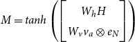
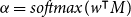
 \begin{align} M &= tanh\left( \begin {bmatrix} W_h H \\ W_v v_a \otimes e_N \\ \end {bmatrix} \right) \nonumber\\[3pt] \alpha &= softmax(w^\intercal M) \nonumber\\[3pt] r &= H \alpha ^\intercal\end{align}
where $M \in \mathbb{R}^{(d+d_a)\times N}$
,
$M \in \mathbb{R}^{(d+d_a)\times N}$
, $\alpha \in \mathbb{R}^N$
,
$\alpha \in \mathbb{R}^N$
, $r \in \mathbb{R}^d$
,
$r \in \mathbb{R}^d$
, $W_h \in \mathbb{R}^{d\times d}$
,
$W_h \in \mathbb{R}^{d\times d}$
, $W_v \in \mathbb{R}^{d_a\times d_a}$
,
$W_v \in \mathbb{R}^{d_a\times d_a}$
, $w \in \mathbb{R}^{d + d_a}$
.
$w \in \mathbb{R}^{d + d_a}$
. $v_a \otimes e_N = [v_a, v_a, \ldots, v_a]$
represents the operation that repeatedly concatenates
$v_a \otimes e_N = [v_a, v_a, \ldots, v_a]$
represents the operation that repeatedly concatenates $v_a$
for
$v_a$
for $N$
times. Regarding the lexical inputs, let
$N$
times. Regarding the lexical inputs, let $V_l \in \mathbb{R}^{n \times N}$
be the lexical feature matrix of the sentence,
$V_l \in \mathbb{R}^{n \times N}$
be the lexical feature matrix of the sentence, $V_l$
then is transformed linearly (Equation (2)) by:
$V_l$
then is transformed linearly (Equation (2)) by:
 \begin{equation} L = W_l \cdot V_l \end{equation}
where $L \in \mathbb{R}^{d \times N}, W_l \in \mathbb{R}^{d \times n}$
. Later, the attention vector
$L \in \mathbb{R}^{d \times N}, W_l \in \mathbb{R}^{d \times n}$
. Later, the attention vector $\alpha$
learned from the concatenation of
$\alpha$
learned from the concatenation of $H$
and
$H$
and $v_a \otimes e_N$
is applied on
$v_a \otimes e_N$
is applied on $L$
to obtain a weighted representation of the lexical features (Equation (3)):
$L$
to obtain a weighted representation of the lexical features (Equation (3)):
 \begin{equation} l = L \cdot \alpha ^\intercal \end{equation}
where $l \in \mathbb{R}^d, \alpha \in \mathbb{R}^N$
. Finally, the mixed final representation of all inputs
$l \in \mathbb{R}^d, \alpha \in \mathbb{R}^N$
. Finally, the mixed final representation of all inputs $h^*$
is updated and passed to the output layer by:
$h^*$
is updated and passed to the output layer by:
 \begin{equation} h^* = tanh(W_p r + W_x h_N + W_o l) \end{equation}
 \begin{equation} \hat{y} = softmax(W_s h^* + b_s) \end{equation}
where $W_o \in \mathbb{R}^{d \times d}$
is a projection parameter as
$W_o \in \mathbb{R}^{d \times d}$
is a projection parameter as $W_p$
and
$W_p$
and $W_x$
;
$W_x$
; $W_s$
and
$W_s$
and $b_s$
are weights and biases in the output layer. The same loss function as the baseline is used to train the model:
$b_s$
are weights and biases in the output layer. The same loss function as the baseline is used to train the model:
 \begin{equation} loss = - \sum _i y_i log(\hat{y}_i) + \lambda \|\boldsymbol{\Theta }\|_2^2 \end{equation}
where $i$
is the number of classes (ternary classification in our experiments).
$i$
is the number of classes (ternary classification in our experiments). $\lambda$
is the hyperparameter for
$\lambda$
is the hyperparameter for $L_2$
regularization. And
$L_2$
regularization. And $\boldsymbol{\Theta }$
is the parameter set of the network to be regularized; compared to the baseline, new parameters
$\boldsymbol{\Theta }$
is the parameter set of the network to be regularized; compared to the baseline, new parameters $W_l$
and
$W_l$
and $W_o$
are added to
$W_o$
are added to $\boldsymbol{\Theta }$
.
$\boldsymbol{\Theta }$
.
Lexicon
In order to have a broader coverage of the vocabulary, we first build our lexicon from 4 existing lexicons by merging them into one, namely MPQA Footnote a , Opinion Lexicon Footnote b , OpeNER Footnote c, and Vader Footnote d . There is no specific reason for us to select any particular lexicon; as all four lexicons are open source, easily accessible, and domain independent, we select them out of convenience.
After gathering the resources, we have to standardize the polarities in these lexicons as they are not annotated with the same standard. Specifically, for lexicons with categorical labels such as negative, weakneg, neutral, both, positive, we convert them into numerical values as {–1.0, –0.5, 0.0, 0.0, 1.0}, respectively. On the other hand, regarding lexicons with real number annotations, for each lexicon, we adopt the annotated value normalized by the maximum absolute polarity value in that lexicon. Namely, let $\boldsymbol{p} \in \{p_1, p_2, \ldots, p_n\}$
be the set of unique numerical polarities of a given lexicon, the normalized polarity
$\boldsymbol{p} \in \{p_1, p_2, \ldots, p_n\}$
be the set of unique numerical polarities of a given lexicon, the normalized polarity $p_i$
is computed as (Equation (7)):
$p_i$
is computed as (Equation (7)):
 \begin{equation} p_i = \frac{p_i}{max(|\boldsymbol{p}|)} \:\:\:\: \forall _i \in \{1, 2, \ldots, n\} \end{equation}
Finally, all lexicons are merged into a union $U$
, where each word
$U$
, where each word $w_l \in U$
has an associated vector
$w_l \in U$
has an associated vector $v_l \in \mathbb{R}^n$
(
$v_l \in \mathbb{R}^n$
( $n$
is the number of lexicons) that encodes the numerical polarity of each lexicon. In case of any lexicon that does not contain a certain entry, the average polarity value of all available lexicons is used to fill in the missing one. A
$n$
is the number of lexicons) that encodes the numerical polarity of each lexicon. In case of any lexicon that does not contain a certain entry, the average polarity value of all available lexicons is used to fill in the missing one. A $n$
dimensional zero vector is supplemented for words not in
$n$
dimensional zero vector is supplemented for words not in $U$
. As an example, Table 1 shows a small portion of the merged lexicon.
$U$
. As an example, Table 1 shows a small portion of the merged lexicon.
Table 1. Example of the merged lexicon $U$
$U$

3.2 Attention regularization
Since the attention vector is learned purely based on the training examples, it is possible that it is over-fitted in some cases, causing the network to overlook some key information. A graphical representation of this effect is shown in Figure 10 below: the attention weights in ATLX are less sparse across the sentence, while the ones in the baseline are focusing only on the last parts of the sentence (details will be discussed in Section 4.2). In addition, we observe that the distribution of all the attention weights in ATLX has a lower varianceFootnote e than in the baseline. Note that the attention weights sum up to one, so when weights are closer to mean (not zero), the standard deviation is smaller; on the other hand, when most weights are close to zero and the rest few weights are close to one, the standard deviation is larger.
Thus, we propose a simple method to validate our hypothesis, which consists of adding into the loss function a second regularizer that governs the attention distribution, namely a standard deviation regularizer or a negative entropy regularizer. The idea is to avoid the attention vector being overly sparse by having large weights in few positions; instead, it is preferred to have higher weight values for more positions, that is, to have an attention vector with more spread out weights. Formally, the attention regularized loss function is defined as:
 \begin{equation} loss = - \sum _i y_i log(\hat{y}_i) + \lambda \|\boldsymbol{\Theta }\|_2^2 + \epsilon \: \Omega (\boldsymbol{\alpha }) \end{equation}
Compared to the loss function in ATLX (Equation (6)), a second regularization term $\epsilon \: \Omega (\boldsymbol{\alpha })$
is added, where
$\epsilon \: \Omega (\boldsymbol{\alpha })$
is added, where $\epsilon$
is the hyperparameter for the attention regularizer (always positive);
$\epsilon$
is the hyperparameter for the attention regularizer (always positive); $\Omega$
stands for the regularization function defined in Equations (9) or (10), and
$\Omega$
stands for the regularization function defined in Equations (9) or (10), and $\alpha$
is the attention vector, that is, the distribution of attention weights.
$\alpha$
is the attention vector, that is, the distribution of attention weights.
Regarding $\Omega$
itself, we experiment two different regularizers in our experiments: one uses the standard deviation of
$\Omega$
itself, we experiment two different regularizers in our experiments: one uses the standard deviation of $\alpha$
defined in Equation (9) and another one uses the negative entropy of
$\alpha$
defined in Equation (9) and another one uses the negative entropy of $\alpha$
defined in Equation (10).
$\alpha$
defined in Equation (10).
Standard deviation regularizer
 \begin{equation} \Omega (\alpha ) = \sigma (\alpha ) = \sqrt{\frac{1}{N} \sum _i^N(\alpha _i - \mu )^2} \end{equation}
Negative entropy regularizer
 \begin{align}ent(\alpha ) &= - \sum _i^N \alpha _i log(\alpha _i) \nonumber \\[3pt] \Omega (\alpha ) &= - ent(\alpha ) \end{align}
3.3 Sentiment induction
3.3.1 Sentiment domain adaptation
Vector-based domain adaptation nethod
In our experiments, we take the approach by Mudinas et al. (Reference Mudinas, Zhang and Levene2019) to perform sentiment domain adaptation, who discovered that the distributed word representations in fact form distinct clusters for opposite sentiments, and this behavior in general holds across different domains. In other words, in the vector space shaped by a domain-specific corpus, positive words are closer to each other than they are to negative words, and the same behavior is expected in other domains. Thus, a probabilistic word classifier can be trained on a set of seed words (a number of predefined words which have consistent sentiment behavior in different domains, e.g., “good” and “bad)”, and this classifier can be used to induce the generic sentiment lexicon by predicting the word polarity in a new domain given its domain-specific word embeddings.
Specifically, we use the domain-specific word embeddingsFootnote
f
learned from Amazon electronics review corpus and a set of seed words (listed in Table 2) to form a set of training examples. Each example is composed by $(x, y)$
pairs where
$(x, y)$
pairs where $x \in \mathbb{R}^{500}$
is the 500 dimensional domain-specific word vector, and
$x \in \mathbb{R}^{500}$
is the 500 dimensional domain-specific word vector, and $y$
is the seed word polarity as a label. Next, we train a SVM classifier (Pedregosa et al. Reference Pedregosa, Varoquaux, Gramfort, Michel, Thirion, Grisel, Blondel, Prettenhofer, Weiss, Dubourg, Vanderplas, Passos, Cournapeau, Brucher, Perrot and Duchesnay2011) with rbf kernel and
$y$
is the seed word polarity as a label. Next, we train a SVM classifier (Pedregosa et al. Reference Pedregosa, Varoquaux, Gramfort, Michel, Thirion, Grisel, Blondel, Prettenhofer, Weiss, Dubourg, Vanderplas, Passos, Cournapeau, Brucher, Perrot and Duchesnay2011) with rbf kernel and $C=10$
as a regularization parameter. Finally, we use the trained classifier to predict the polarity of generic lexicon words (
$C=10$
as a regularization parameter. Finally, we use the trained classifier to predict the polarity of generic lexicon words ( $U$
described in Section 3.1.2). When predicting, a confidence threshold
$U$
described in Section 3.1.2). When predicting, a confidence threshold $t=0.7$
is applied to reduce noise; that is, the polarity of the generic lexicon is updated only when
$t=0.7$
is applied to reduce noise; that is, the polarity of the generic lexicon is updated only when $p \geq t$
where
$p \geq t$
where $p$
is the maximum predicted probability of the classifier.
$p$
is the maximum predicted probability of the classifier.
Table 2. Seed words and word counts used for domain adaptation

We use this approach to convert $U$
from a generic domain lexicon into a domain-specific one (Amazon electronic reviews). Then, we apply it in ATLX and compare it with applying a gold domain-specific lexicon constructed by ourselves (Section 6). We evaluate the performance gain of each lexicon when applied in the ATLX model to understand the limit of domain adaptation.
$U$
from a generic domain lexicon into a domain-specific one (Amazon electronic reviews). Then, we apply it in ATLX and compare it with applying a gold domain-specific lexicon constructed by ourselves (Section 6). We evaluate the performance gain of each lexicon when applied in the ATLX model to understand the limit of domain adaptation.
In addition, compared to the binary classification originally applied in Mudinas et al. (Reference Mudinas, Zhang and Levene2018) using only positive and negative seed words, we find that the binary classification would misclassify obvious neutral words, even when a $0.7$
confidence threshold is applied. For example, “really,” “very,” and “thought” are predicted to be negative, positive, and negative, respectively. Thus, to further reduce noise, we introduce an additional set of 35 neutral seed words (Table 2) to perform ternary classification instead of binary.
$0.7$
confidence threshold is applied. For example, “really,” “very,” and “thought” are predicted to be negative, positive, and negative, respectively. Thus, to further reduce noise, we introduce an additional set of 35 neutral seed words (Table 2) to perform ternary classification instead of binary.
Gold lexicon
To better interpret the experimental results and understand the limit of domain adaptation, we find the intersection $I$
(839 elements) between the set of generic lexicon entries
$I$
(839 elements) between the set of generic lexicon entries $G$
(13,297 elements) and the set of the corpus vocabulary
$G$
(13,297 elements) and the set of the corpus vocabulary $V$
(2,965 elements), where
$V$
(2,965 elements), where $I = G \cap V$
. Then, we label
$I = G \cap V$
. Then, we label $I$
to be the gold lexicon of the electronics review domain, where polarities positive, neutral, and negative are annotated as numerical values:
$I$
to be the gold lexicon of the electronics review domain, where polarities positive, neutral, and negative are annotated as numerical values: $1$
,
$1$
, $0$
and
$0$
and $-1$
, respectively. Three principles are defined as annotation guidelines:
$-1$
, respectively. Three principles are defined as annotation guidelines:
-
(1) Domain first: prioritize the most common meaning of the word in the current domain. For example, in the electronics or laptops review domain, “fallout” or “excel” are neutral proper nouns referring to a video game and a software; however, under generic context “fallout” and “excel” are marked as negative and positive. Similarly, nouns such as “brightness,” “durability” and “security” have positive sentiment under generic context, but here they in fact refer to neutral product aspects.
-
(2) Neutral adverbs: adverbs in general should be neutral especially when they can be used to modify both positive and negative words. For example “definitely,” “fairly” and “truly” can all express opposite sentiment depends on the word that follows (“definitely great ” vs “definitely garbage ”).
-
(3) Neutral ambiguity: ambiguous context-dependent words should be neutral in the lexicon, in order to avoid feeding confusing information to the model. For instance, “cheap price” carries positive sentiment while “cheap plastic” is definitely negative. Other examples are: “black screen” vs “black macbook”; “loud speaker” vs “loud click”; “low price” vs “low grade.”
3.3.2 Sentiment aspect adaptation
To deal with the aspect-dependent problem (e.g., “cheap price” vs “cheap plastic”), we adopt a similar approach to the domain adaptation method described in Section 3.3.1. More specifically, we build a set of training data using the same seed words shown in Table 2: the domain-specific word embeddings of each word is merged with the aspect embeddings of each aspect word, the merged word vector serve as input features to the classifier; and the seed words labels are served as classes. Then, the same SVM classifier as for domain adaptation (Section 3.3.1) is trained and used to update the generic lexicon $U$
given its word embeddings and aspect embeddings as joint inputs.
$U$
given its word embeddings and aspect embeddings as joint inputs.
Formally, let $A$
be the set of 9 aspect words in which each word is
$A$
be the set of 9 aspect words in which each word is $A=\{$
“connectivity,” “design,” “general,” “miscellaneous,” “performance,” “portability,” “price,” “quality,” “usability”
$A=\{$
“connectivity,” “design,” “general,” “miscellaneous,” “performance,” “portability,” “price,” “quality,” “usability” $\}$
. Let
$\}$
. Let $v_a^{\,j}$
be the word vector of an aspect word
$v_a^{\,j}$
be the word vector of an aspect word $j \in A$
, where all word vectors are learned from the Amazon electronics review corpus, same as the domain adaptation method. Let
$j \in A$
, where all word vectors are learned from the Amazon electronics review corpus, same as the domain adaptation method. Let $S$
be the set of seed words in Table 2 and
$S$
be the set of seed words in Table 2 and $v_s^i$
be the domain-specific word embeddings of a seed word
$v_s^i$
be the domain-specific word embeddings of a seed word $i \in S$
.
$i \in S$
. $y_i$
be the label of the word
$y_i$
be the label of the word $i$
from
$i$
from $S$
, namely positive, neutral, or negative. Thus for each training example
$S$
, namely positive, neutral, or negative. Thus for each training example $(x_{ij}, y_i)$
, we have
$(x_{ij}, y_i)$
, we have
 \begin{equation*}x_{ij} = v_s^i \oplus v_a^{\,j} \:\:\:\: \forall _j \in A\end{equation*}
where $\oplus$
is an operation of concatenation, summation, or mean of two vectors
$\oplus$
is an operation of concatenation, summation, or mean of two vectors $v_s^i$
and
$v_s^i$
and $v_a^j$
. This is equivalent to a Cartesian product between
$v_a^j$
. This is equivalent to a Cartesian product between $S$
and
$S$
and $A$
, and for each element in the output, we concatenate (or sum, or average) their corresponding domain-specific word vectors as input features.
$A$
, and for each element in the output, we concatenate (or sum, or average) their corresponding domain-specific word vectors as input features.
Then, these training examples are used to train a SVM classifier same as the domain adaptation method. And finally, the trained classifier is used to predict the polarity of a tuple consisting of the domain-specific word vector of a given word in $U$
and the aspect vector of any aspect from
$U$
and the aspect vector of any aspect from $A$
. When the predicted probability is larger than the threshold
$A$
. When the predicted probability is larger than the threshold $t$
, the polarity of that word-aspect pair is modified. The final aspect-specific lexicon is essentially a dictionary with keys as the Cartesian product of
$t$
, the polarity of that word-aspect pair is modified. The final aspect-specific lexicon is essentially a dictionary with keys as the Cartesian product of $U$
and
$U$
and $A$
. And when used in the ABSA system, the polarity of a word is given by the expanded lexicon based on the input word and its associated aspect. Same as the domain adaptation method described in Section 3.3.1, we train a SVM classifier (Pedregosa et al., Reference Pedregosa, Varoquaux, Gramfort, Michel, Thirion, Grisel, Blondel, Prettenhofer, Weiss, Dubourg, Vanderplas, Passos, Cournapeau, Brucher, Perrot and Duchesnay2011) with rbf kernel and
$A$
. And when used in the ABSA system, the polarity of a word is given by the expanded lexicon based on the input word and its associated aspect. Same as the domain adaptation method described in Section 3.3.1, we train a SVM classifier (Pedregosa et al., Reference Pedregosa, Varoquaux, Gramfort, Michel, Thirion, Grisel, Blondel, Prettenhofer, Weiss, Dubourg, Vanderplas, Passos, Cournapeau, Brucher, Perrot and Duchesnay2011) with rbf kernel and $C=10$
as a regularization parameter, and the threshold
$C=10$
as a regularization parameter, and the threshold $t=0.7$
is used.
$t=0.7$
is used.
4. Experiments
4.1 Lexicon enhancement (ATLX)
4.1.1 Datasets
We conduct our experiments on the SemEval 2014 Task 4, restaurant domain dataset, same as Wang et al. (Reference Wang, Huang, Zhao and Zhu2016). The data consist of reviews of restaurants with predefined aspects: {food, price, service, ambience, miscellaneous} and associated polarities: {positive, neutral, negative}. The objective is to predict the polarity given a sentence and an aspect. For instance, given a review sentence “The restaurant was too expensive,” the model should identify the negative polarity associated with the aspect price. In total, there are 3,518 training examples and 973 test examples in the corpus. Table 3 shows the distribution of aspects per label for both training and test data.
Table 3. Distribution of aspects by label and train/test split in the SemEval 2014 Task4, restaurant domain dataset.

In addition, we also reproduce our experiments on the SemEval 2015 Task 12, laptop domain dataset. The dataset consists of reviews of laptops with annotated entity-attribute pairs such as: {LAPTOP#GENERAL, KEYBOARD#QUALITY, LAPTOP#PRICE, …} and associated polarities: {positive, neutral, negative}. In order to have comparable results with the SemEval 2014 dataset, we simplify the attribute annotations to {general, performance, design, usability, portability, price, quality, miscellaneous, connectivity} and use them as aspects. Together, there are 1973 training examples and 949 test examples in the corpus. Details of the corpus statistics are shown in Table 4.
Table 4. Distribution of aspects by label and train/test split in the SemEval 2015 Task12, laptop domain dataset.

Regarding the word vectors, we use pre-trained word embeddings to initialize the parameters in the embedding layer of our model. Namely, the 300 dimensional GloveFootnote g vectors trained on 840B tokens are used for the ATLX model.
4.1.2 Lexicons
As shown in Table 5, we merge four existing and online available lexicons into one. The merged lexicon $U$
as described in Section 3.1.2 is used for our experiments. After the union, the following post-process is carried out:
$U$
as described in Section 3.1.2 is used for our experiments. After the union, the following post-process is carried out: $\{bar, try, too\}$
are removed from
$\{bar, try, too\}$
are removed from $U$
since they are unreasonably annotated as negative by MPQA and Opener;
$U$
since they are unreasonably annotated as negative by MPQA and Opener; $\{n't, not\}$
are added to
$\{n't, not\}$
are added to $U$
with
$U$
with $-1$
polarity for negation as we have observed cases in early experiments where the model struggles to identify negation after lexicon integration.
$-1$
polarity for negation as we have observed cases in early experiments where the model struggles to identify negation after lexicon integration.
Table 5. Lexicon statistics of positive, neutral, negative words, and number of words covered in corpus.

4.1.3 ATLX variants
In order to effectively merge lexicon information to the baseline system, apart from the ATLX model described in Section 3.1.2, we have designed a set of variants as well, namely a variety of ways slightly different from ATLX to merge lexicon information into the system.
Variant 1
Recall that in ATLX (Equation (3), Section 3.1.2), the lexical representation $l$
is obtained by applying the attention weights
$l$
is obtained by applying the attention weights $\alpha$
on the transformed lexical features
$\alpha$
on the transformed lexical features $L$
:
$L$
:
 \begin{equation*}l = L \cdot \alpha ^\intercal \end{equation*}
Here, instead of applying the attention vector $\alpha$
, a linear transformation is adopted to obtain
$\alpha$
, a linear transformation is adopted to obtain $l$
(Equation (11)):
$l$
(Equation (11)):
 \begin{equation} l = L \cdot w_{v1} \end{equation}
where $L \in \mathbb{R}^{d \times N}$
,
$L \in \mathbb{R}^{d \times N}$
, $w_v \in \mathbb{R}^{N}$
, and
$w_v \in \mathbb{R}^{N}$
, and $l \in \mathbb{R}^d$
.
$l \in \mathbb{R}^d$
.
Variant 2
Recall that in ATLX (Equation (1), Section 3.1.2), the attention vector $\alpha$
is computed with the concatenation of transformed hidden states
$\alpha$
is computed with the concatenation of transformed hidden states $H$
and the repeated aspect vectors
$H$
and the repeated aspect vectors $v_a$
as input:
$v_a$
as input:
 \begin{equation*} M = tanh\left( \begin {bmatrix} W_h H \\ W_v v_a \otimes e_N \\ \end {bmatrix} \right) \end{equation*}
 \begin{equation*}\alpha = softmax(w^\intercal M)\end{equation*}
Here, we add a third input to compute $\alpha$
, which is the lexical features
$\alpha$
, which is the lexical features $L$
projected by some network parameter
$L$
projected by some network parameter $W_{v2}$
:
$W_{v2}$
:
 \begin{equation} M = tanh\left( \begin{bmatrix} W_h H \\ W_v v_a \otimes e_N \\ W_{v2} L\\ \end{bmatrix} \right) \end{equation}
 \begin{equation*}\alpha = softmax(w^\intercal M)\end{equation*}
where $L \in \mathbb{R}^{d \times N}$
,
$L \in \mathbb{R}^{d \times N}$
, $W_{v2} \in \mathbb{R}^{d \times d}$
, and
$W_{v2} \in \mathbb{R}^{d \times d}$
, and $M \in \mathbb{R}^{(d+d_a+d)\times N}$
.
$M \in \mathbb{R}^{(d+d_a+d)\times N}$
.
Variant 3
Recall that in ATLX (Equation (4), Section 3.1.2), the final representation $h^*$
is composed by the summation of three lower level representations:
$h^*$
is composed by the summation of three lower level representations: $r$
,
$r$
, $h_N$
, and
$h_N$
, and $l$
:
$l$
:
 \begin{equation*}h^* = tanh(W_p r + W_x h_N + W_o l)\end{equation*}
Here instead of summation, a concatenation of three elements is made to form the final representation:
 \begin{equation} h^* = tanh\left( \begin{bmatrix} W_p r \\ W_x h_N \\ W_o l\\ \end{bmatrix} \right) \end{equation}
where $r \in \mathbb{R}^d$
,
$r \in \mathbb{R}^d$
, $l \in \mathbb{R}^d$
,
$l \in \mathbb{R}^d$
, $h_N \in \mathbb{R}^d$
, and
$h_N \in \mathbb{R}^d$
, and $h^* \in \mathbb{R}^{3d}$
.
$h^* \in \mathbb{R}^{3d}$
.
Variant 4
Similar to Variant 3, compared to ATLX where the final representation is obtained through the summation of three lower level representations, here we use a different approach to compute $h^*$
. Inspired by the attention mechanism, we would like to have a second attention mechanism here to weight the lower level representations when aggregating the final representation. This way, the model would be able to weight different information sources accordingly as lexical features are not always available (words outside of the lexicon are treated as neutral as described in Section 3.1.2).
$h^*$
. Inspired by the attention mechanism, we would like to have a second attention mechanism here to weight the lower level representations when aggregating the final representation. This way, the model would be able to weight different information sources accordingly as lexical features are not always available (words outside of the lexicon are treated as neutral as described in Section 3.1.2).
Formally, let $H^*$
be the concatenation of
$H^*$
be the concatenation of $W_p r + W_x h_N$
and
$W_p r + W_x h_N$
and $W_o l$
(Equation (14)), a new attention vector
$W_o l$
(Equation (14)), a new attention vector $\beta$
(Equation (15)) is learned and applied back to
$\beta$
(Equation (15)) is learned and applied back to $H^*$
to obtain the final representation (Equation (16)):
$H^*$
to obtain the final representation (Equation (16)):
 \begin{equation} H^* = tanh\!\left( \begin{bmatrix} W_p r + W_x h_N, W_o l\\ \end{bmatrix} \right) \end{equation}
 \begin{equation} \beta = softmax(w_b^\intercal H) \end{equation}
 \begin{equation} h^* = H \beta ^\intercal \end{equation}
where $H^* \in \mathbb{R}^{d \times 2}$
,
$H^* \in \mathbb{R}^{d \times 2}$
, $w_b \in \mathbb{R}^d$
,
$w_b \in \mathbb{R}^d$
, $\beta \in \mathbb{R}^2$
,
$\beta \in \mathbb{R}^2$
, $h^* \in \mathbb{R}^d$
.
$h^* \in \mathbb{R}^d$
.
4.1.4 Evaluation
In our experiments, we use cross-validation (CV) to evaluate the performance of each model. Specifically, the training set is randomly shuffled and split into six-folds with a fixed random seed. According to the codeFootnote
h
released by Wang et al. (Reference Wang, Huang, Zhao and Zhu2016), a development set containing 528 examples is used in the implementation of AT-LSTM, which is roughly $\frac{1}{6}$
of the training corpus. In order to remain faithful to the original implementation, we thus evaluate our model with a CV of six-folds.
$\frac{1}{6}$
of the training corpus. In order to remain faithful to the original implementation, we thus evaluate our model with a CV of six-folds.
Table 6 shows the evaluation results of the baseline system, ATLX, and four variants of ATLX on the SemEval14 restaurant dataset. Compared to the baseline system, ATLX improves on both CV and test sets in terms of average accuracy. However, the significance test comparing the performance distribution of the ATLX model and the baseline on the test set does not suggest a statistically significant improvement (p-value = $0.052 \gt 0.05$
). Nevertheless, the analysis in Section 4.1.5 does support the effectiveness of the lexicon enhancement. Meanwhile, the four variants of ATLX cannot achieve a superior performance compared to ATLX, and some even decrease compared to the baseline. For instance, both variant 1 and variant 2 improve slightly on the CV sets compared to the baseline; however, only variant 2 improves on the test set as well while variant 1 suffers a drop back. On the other hand, both variant 3 and variant 4 show an inferior performance compared to the baseline on both CV sets and test set, where variant 4 suffers the largest decrease. In Section 4.1.6, we will discuss some potential insights learned from these failed experiments.
$0.052 \gt 0.05$
). Nevertheless, the analysis in Section 4.1.5 does support the effectiveness of the lexicon enhancement. Meanwhile, the four variants of ATLX cannot achieve a superior performance compared to ATLX, and some even decrease compared to the baseline. For instance, both variant 1 and variant 2 improve slightly on the CV sets compared to the baseline; however, only variant 2 improves on the test set as well while variant 1 suffers a drop back. On the other hand, both variant 3 and variant 4 show an inferior performance compared to the baseline on both CV sets and test set, where variant 4 suffers the largest decrease. In Section 4.1.6, we will discuss some potential insights learned from these failed experiments.
Table 6. Mean accuracy and standard deviation ( $\sigma$
) of cross-validation results on six-folds of development sets and one holdout test set of the SemEval14, restaurant dataset. Note that in our replicated baseline system, the cross-validation performance on the test set ranges from 80.06 to 83.45; in Wang et al. (Reference Wang, Huang, Zhao and Zhu2016), 83.1 was reported.
$\sigma$
) of cross-validation results on six-folds of development sets and one holdout test set of the SemEval14, restaurant dataset. Note that in our replicated baseline system, the cross-validation performance on the test set ranges from 80.06 to 83.45; in Wang et al. (Reference Wang, Huang, Zhao and Zhu2016), 83.1 was reported.

To further validate the effectiveness of ATLX, we conduct similar experiments on the SemEval15 laptop dataset. More specifically, we apply both the baseline and the ATLX model on the SemEval15 dataset and see if a similar improvement can be observed. Table 7 shows the evaluation results of the two models on both datasets. From the table, we can see that similar to the SemEval14 dataset, compared to the baseline, ATLX improves on both the CV sets and the test set of the SemEval15 dataset as well. In addition, the significance test comparing the performance distribution of the ATLX model and the baseline on the test set suggests that they are significant (p-value = $0.018 \lt 0.05$
).
$0.018 \lt 0.05$
).
Table 7. Mean accuracy and standard deviation ( $\sigma$
) of cross-validation results on six-folds of development sets and one holdout test set. Evaluated on the SemEval14, restaurant dataset and the SemEval15, laptop dataset.
$\sigma$
) of cross-validation results on six-folds of development sets and one holdout test set. Evaluated on the SemEval14, restaurant dataset and the SemEval15, laptop dataset.

It is worth mentioning that the results on the SemEval15 dataset have higher variance than the SemEval14 dataset ( $\sigma ^{CV}$
of the baseline and ATLX on the SemEval15 dataset are both above
$\sigma ^{CV}$
of the baseline and ATLX on the SemEval15 dataset are both above $2.0$
, compared to the ones in SemEval14 which are both below
$2.0$
, compared to the ones in SemEval14 which are both below $1.5$
), and the variance improvements of the proposed methods are only observed in the SemEval14 dataset. Given the fact that both datasets are not large in terms of scale under modern deep learning standards, and the SemEval15 dataset is even smaller than the SemEval14 dataset, it is hard to draw a strong conclusion here.
$1.5$
), and the variance improvements of the proposed methods are only observed in the SemEval14 dataset. Given the fact that both datasets are not large in terms of scale under modern deep learning standards, and the SemEval15 dataset is even smaller than the SemEval14 dataset, it is hard to draw a strong conclusion here.
4.1.5 Qualitative analysis
Lexicon size
To further explore the impact of adding lexical features into the system, we conduct another support experiment focusing on the changes caused by the size of the lexicon.
As described in Section 3.1.2, neutral polarity is supplied for words outside the lexicon. Let $u \in U$
be the subset of lexicon entries where
$u \in U$
be the subset of lexicon entries where $u = U \cap V$
and
$u = U \cap V$
and $V$
is the vocabulary of the corpus. In Table 5, the size of
$V$
is the vocabulary of the corpus. In Table 5, the size of $u$
in our experiment is
$u$
in our experiment is $1234$
. In order to experiment with the impact caused by the size of the lexicon, we randomly shuffle
$1234$
. In order to experiment with the impact caused by the size of the lexicon, we randomly shuffle $u$
and perform the same CV evaluation on ATLX with an increasing size of
$u$
and perform the same CV evaluation on ATLX with an increasing size of $u$
by a step of 200. Figure 3 shows the CV performance on the test set.
$u$
by a step of 200. Figure 3 shows the CV performance on the test set.
In general, we can see that larger size of $u$
tends to yield better overall performance but with an exception of size
$u$
tends to yield better overall performance but with an exception of size $1000$
, where the performance becomes more variant.
$1000$
, where the performance becomes more variant.
Lexicon dimensions
As shown in Table 8, the dimension of the lexical feature affects the performance of the model to some extent. The best performance comes from $n=3$
, that is when using only 3 columns of the merged lexicon
$n=3$
, that is when using only 3 columns of the merged lexicon $U$
, which is the result reported as ATLX in Table 6 and others that follow. Although the difference between ATLXn = 3 and ATLXn = 4 is negligible and the performance seems linear with respect to
$U$
, which is the result reported as ATLX in Table 6 and others that follow. Although the difference between ATLXn = 3 and ATLXn = 4 is negligible and the performance seems linear with respect to $n$
, it would be safer to select
$n$
, it would be safer to select $n$
through tuning.
$n$
through tuning.
Table 8. ATLX lexicon dimension experiments on SemEval14, restaurant domain dataset.


Figure 3. ATLX cross-validation results on test set with increasing lexicon size on SemEval14, restaurant domain dataset.
Case studies
Given results from the previous section, the overall performance of the ATLX model is enhanced compared to the baseline, and more importantly, by leveraging lexical features independent from the training data, the model becomes more robust and flexible. For instance in Figure 4, although the baseline is able to pay relatively high attention to the word “disappointed” and “dungeon,” it is not able to recognize these words as clear indicators of negative polarity, while ATLX is able to correctly predict negative for both examples. It is also interesting to see that in the second example, the attention shifts to the word “dungeon” in ATLX compared to the baseline, suggesting that the model is able to take advantage of the extra information provided by the lexicon.

Figure 4. Baseline (“Base”) and ATLX comparison (1/6); baseline predicts positive (“Pos”) for both examples, while the gold labels are negative (“Neg”) for all. In the rows annotated as “Base” and “ATLX,” the numbers represent the attention weights of each model when predicting. Note that they do not sum up to 1 in the Figure because predictions are done in a batch with padding positions in the end which are not shown in the Figure. The rows annotated as “Lexicon” indicate the average polarity per word given by $U$
as described in Section 3.1.2. In some of the following plots, the neutral polarity is annotated as (“Neu”).
$U$
as described in Section 3.1.2. In some of the following plots, the neutral polarity is annotated as (“Neu”).
In Figure 5, we can see another case in which after introducing the lexicon, the model is able to attend more to a keyword and makes the correct prediction. Specifically, given the aspect service, the baseline is not able to predict the correct negative label although the clause “the service is terrible” has been given relatively higher weights. On the other hand, the weight of the opinion word “terrible” is doubled in ATLX with the polarity of the word “terrible” fed to the model.

Figure 5. Baseline and ATLX comparison (2/6).
In Figure 6, we can see a rather simple case, in which the baseline predicts incorrectly the neutral label. However, in ATLX, although the distribution of the attention weights is similar to the baseline, the model now can correctly predict positive given the aspect food.

Figure 6. Baseline and ATLX comparison (5/6). Baseline predicts neutral (“Neu”).
Although the general performance of ATLX is better than the baseline, there are also cases where the lexicon-enhanced model performs worse than the baseline. By adding lexical features in the system, it is inevitable to introduce noise, and such noise may confuse the model.
For example in Figure 7, both the baseline and ATLX are able to pay relatively high attention to the second clause: “definitely the place to be”; however, ATLX is not able to identify the positive polarity given the miscellaneous aspect. It is worth mentioning that the polarities of all three non-neutral words given by the lexicon would be more reasonable to be considered as neutral. Such noise from the lexicon can produce a negative effect on the ATLX model.

Figure 7. Baseline and ATLX comparison (4/6).
Similarly, in Figure 8, given the aspect miscellaneous, the ATLX model fails to identify the neutral polarity. Compared to the baseline, ATLX “focuses” more on the word “promptly,” which carries a positive sentiment according to the lexicon. Under this context, it is reasonable that “seated promptly” refers to good fast service because there was no need to wait. However, it is indeed neutral regarding the aspect miscellaneous. Nevertheless, the words “close” and “dance” are marked as negative and positive by the lexicon, which is disputable.

Figure 8. Baseline and ATLX comparison (5/6).
A slightly more complex example can be found in Figure 9, where a comparative opinion is expressed on top of a positive opinion. In fact, comparative opinions are studied as a sub-field of sentiment analysis due to their complex structure (Liu Reference Aue and Gamon2012). In this case, the baseline model predicts correctly and the ATLX model seems to be affected by the number of positive and negative opinion words marked by the lexicon.

Figure 9. Baseline and ATLX comparison (6/6).
4.1.6 Discussion
Regarding the ATLX variants described in Section 4.1.3, apparently none of them achieves a superior performance compared to not only ATLX but also the baseline. Although it is not yet fully understood how DNN work to the finest granularity, recent studies have shown signs of interpretability and explainability (Serrano and Smith Reference Serrano and Smith2019; Madsen et al. Reference Li, Chen, Feng, Ma, Wang and Hovy2021). Here by comparing the difference with the ATLX model, we try to point out some potential insights learned from these experiments.
Compared to ATLX, variant 1 uses a linear transformation to process the lexical features $L$
instead of applying the attention vector on
$L$
instead of applying the attention vector on $L$
(Equation (11)). First, a linear transformation seems to be incapable of efficiently passing lower level information to higher level layers. Second, by applying the attention vector
$L$
(Equation (11)). First, a linear transformation seems to be incapable of efficiently passing lower level information to higher level layers. Second, by applying the attention vector $\alpha$
on
$\alpha$
on $L$
instead of putting
$L$
instead of putting $L$
as input to learn
$L$
as input to learn $\alpha$
, when training the network and updating the parameters, the lexical features still have impact on how
$\alpha$
, when training the network and updating the parameters, the lexical features still have impact on how $\alpha$
will change, and thus, the attention framework is capable of taking into account lexical features as well. Consequently, we observe the impact on attention vectors in ATLX compared to the baseline, which allows it to attend more on key opinion words with sentiment information from the lexical features. In addition, the fact that the attention vector is learned to attend to both the input sentence and the lexical features ensures that when putting them together at later steps, there will be no conflict between these two components and it allows us to obtain a final representation more smoothly.
$\alpha$
will change, and thus, the attention framework is capable of taking into account lexical features as well. Consequently, we observe the impact on attention vectors in ATLX compared to the baseline, which allows it to attend more on key opinion words with sentiment information from the lexical features. In addition, the fact that the attention vector is learned to attend to both the input sentence and the lexical features ensures that when putting them together at later steps, there will be no conflict between these two components and it allows us to obtain a final representation more smoothly.
In variant 2, we add the linearly transformed lexical features $L$
into the input for computing the attention vector
$L$
into the input for computing the attention vector $\alpha$
(Equation (12)). The results in Table 6 show that variant 2 does improve on both the CV sets and the test set compared to the baseline; however, the improvement is not as large as ATLX. One possible reason is that by adding
$\alpha$
(Equation (12)). The results in Table 6 show that variant 2 does improve on both the CV sets and the test set compared to the baseline; however, the improvement is not as large as ATLX. One possible reason is that by adding $L$
into the equation, we have also introduced more model parameters that need to be learned, while the dataset is limited in size and cannot help to train a better model. Meanwhile, the model becomes redundant when trying to obtain the final representation of all inputs as
$L$
into the equation, we have also introduced more model parameters that need to be learned, while the dataset is limited in size and cannot help to train a better model. Meanwhile, the model becomes redundant when trying to obtain the final representation of all inputs as $h^* = tanh(W_p r + W_x h_N + W_o l)$
, where both
$h^* = tanh(W_p r + W_x h_N + W_o l)$
, where both $l$
and
$l$
and $r$
are products of the attention vector
$r$
are products of the attention vector $\alpha$
.
$\alpha$
.
Both variant 3 and variant 4 suffer a performance decrease compared to the baseline. Similarly, instead of summing the lower level representations, they try to concatenate the lower level representations (Equation (13)) or using a weighted sum to combine them (Equation (16)). Concatenation as a commonly used approach to combine the outputs of two hidden layers has been widely used in DNN. However in Table 6, the results suggest that summation yields better results. Similar results can be observed for variant 4, where using weighted sum for combining the sentence representation and lexicon representation does not yield a better performance.
4.2 Attention regularization
4.2.1 Evaluation
As described in Section 3.2, in Figure 10, we can observe that in the baseline system, before adding lexical features, the attention weights are more sparse (i.e., large weights in few positions, small weights close to zero in many positions), and mostly focusing only on the last parts of the sentence. However in the ATLX system, the attention weights are less sparse across the sentence. This sparseness could hurt the model by not passing key information to deeper layers. In this case, the baseline is not able to pay attention to “bad manners,” while the ATLX model can. Since the attention vector is purely learned on the training data, we believe it could be over-fitting. Thus, we design two regularizers (Section 3.2) and try to overcome the over-fitting effect.
Table 9 shows the evaluation results of applying these two regularizers in both the baseline and the ATLX model. Compared to the baseline system on both datasets, by adding attention regularization to the baseline system without introducing lexical features, both the standard deviation regularizer (basestd) and the negative entropy regularizer (baseent-) are able to contribute positively, where baseent- yields the largest improvement. But this is only observed on the test sets of both datasets, the performance on the CV sets of SemEval15 is generally worse than the baseline. However, by combining attention regularization and lexical features together, the model is able to achieve the highest test accuracy in all experiments conducted on both datasets.
Table 9. Comparison between main experiments and attention regularizers. Mean accuracy and standard deviation of cross-validation results on six-folds of development sets and one holdout test set. Evaluated on SemEval14 and SemEval15 dataset.

4.2.2 Discussion
As shown in Figure 10, when comparing ATLX with the baseline, we find that although the lexicon only provides non-neutral polarity information for three words, the attention weights of ATLX are less sparse and more spread out than it is in the baseline. On the other hand, this effect is general as the standard deviation of the attention weights distribution in the test set in ATLX (0.0219) is notably lower compared to the baseline (0.0354).
Thus, it makes us think that the attention weights might be over-fitting in some cases as they are purely learned on training examples. This could cause that by giving too much weight to particular words in a sentence, the network ignores other positions which could provide key information for higher level classification. For instance, the example in Figure 10 shows that the baseline, which predicts positive, is “focusing” on the last parts of the sentence, mostly the word “easy”, while ignoring the “bad manners” coming before, which is key for judging the polarity of the sentence given the aspect service. In contrast, the same baseline model trained with attention regularized by standard deviation is able to correctly predict negative just by “focusing” a little bit more on the “bad manners” part.
However, the hard regularization by standard deviation might not be ideal as the optimal minimum value of the regularizer will imply that all words in the sentence have homogeneous weights, which is the opposite of what the attention mechanism is able to gain.
Regarding the negative entropy regularizer, taking into account that the attention weights are outputs of $softmax$
which is normalized to sum up to 1Footnote
i
, although the minimum value of this term would also imply homogeneous weight of
$softmax$
which is normalized to sum up to 1Footnote
i
, although the minimum value of this term would also imply homogeneous weight of $\frac{1}{N}$
, it is interesting to see that with an almost evenly distributed
$\frac{1}{N}$
, it is interesting to see that with an almost evenly distributed $\alpha$
, the model remains sensitive to few positions with relatively higher weights. For example in Figure 10, the same sentence with negative entropy regularization demonstrates that although most positions are closely weighted, the model is still able to differentiate key positions even with a weight difference of 0.01 and correctly predict negative given the service aspect.
$\alpha$
, the model remains sensitive to few positions with relatively higher weights. For example in Figure 10, the same sentence with negative entropy regularization demonstrates that although most positions are closely weighted, the model is still able to differentiate key positions even with a weight difference of 0.01 and correctly predict negative given the service aspect.
4.3 Sentiment induction
So far, the experiments on ATLX have been using sentiment lexicons in a generic domain; to further improve the system, the idea of domain adaptation comes naturally. Currently, most works on sentiment domain adaptation measure the performance by recreating an existing domain-specific lexicon (Hamilton et al., Reference Hamilton, Clark, Leskovec and Jurafsky2016; Mudinas et al. Reference Mudinas, Zhang and Levene2018). It is less frequent to see how much improvement can actually be gained in an applied case. Thus from an application point of view, we ask the question: how much improvement can we get from the domain-specific lexicon in a lexicon-enhanced neural sentiment analysis system? And what is its limit?
To answer these questions, we first apply the method described in Section 3.3.1 to adapt our generic sentiment lexicon described in Section 3.1.2 to a domain-specific lexicon (electronics review). Then, we experiment with the adapted lexicons by applying them in the ATLX model and test the model performance on the SemEval 2015 laptop domain dataset. To better understand the quality of the adapted lexicon and the performance gain it is able to obtain, we also compare the adapted lexicon with the gold lexicon that we constructed (Section 6). Details of the experimental results are described in Section 4.3.1.
On the other hand, as described in Section 3.3.2, we would like to expand the domain adaptation method and apply it to aspect adaptation. In other words, expand the existing generic lexicon to be aspect-specific. Since there is no gold lexicon to evaluate and compare, we test the quality of the aspect adapted lexicon by applying it in the ATLX model and measuring the performance differences. Details of the experiment will be described in Section 4.3.1.
4.3.1 Evaluation
We experiment the domain adaptation performance on the SemEval 2015 Task 12, laptop dataset, same as the ATLX experiments described in Section 4.1.1.
Same as the ATLX experiments, a CV of six-folds is performed and the average accuracy on both development sets and test set is recorded together with the variance. We also compare the adapted lexicons with the gold lexicon by measuring their accuracy and f-score in both binary and ternary scenarios, where neutral is excluded from binary but included in ternary. Table 10 shows the evaluation results.
Table 10.
(a) ATLX model performance (average cross-validation accuracy and variance) with Domain Adapted Lexicons (DAL) on SemEval15 Task 12, laptop dataset. (b) Accuracy and f-score of DALs measured against the gold lexicon, where binary excludes neutral and ternary does not. The subscripts ${}_{\textrm{bin}}$
and
${}_{\textrm{bin}}$
and ${}_{\textrm{ter}}$
refer to binary classification and ternary classification, respectively.
${}_{\textrm{ter}}$
refer to binary classification and ternary classification, respectively.

Table 11 shows the performance of the aspect adapted lexicons when applied in the ATLX model, together with the model performance of the domain adapted lexicons (DALs) and other variations. The subscripts ${}_{\textrm{add}}$
,
${}_{\textrm{add}}$
, ${}_{\textrm{avg}}$
,
${}_{\textrm{avg}}$
, ${}_{\textrm{concat}}$
correspond to the
${}_{\textrm{concat}}$
correspond to the $\oplus$
operation described in Section 3.3.2, where each of them stands for summation, mean, and concatenation of the domain-specific word vector
$\oplus$
operation described in Section 3.3.2, where each of them stands for summation, mean, and concatenation of the domain-specific word vector $v_s^i$
and the domain-specific aspect vector
$v_s^i$
and the domain-specific aspect vector $v_a^j$
, respectively.
$v_a^j$
, respectively.
Table 11. ATLX model performance (average cross-validation accuracy and variance) with Aspect Adapted Lexicons (AAL) on SemEval15 Task 12, laptop dataset.


Figure 10. Comparison of attention weights between baseline (base), baseline with standard deviation regularizer (basestd), baseline with negative entropy regularizer (baseent-), baseline with positive entropy regularizer (baseent+) and ATLX. Baseline predicts positive while all other models correctly predict negative. The row annotated as “Lexicon” indicates the average polarity given by $U$
. Note that only ATLX takes into account lexical features, the rest do not.
$U$
. Note that only ATLX takes into account lexical features, the rest do not.
4.3.2 Discussion
Sentiment domain adaptation
As shown in Table 10, we observe that in the laptops review domain, the generic lexicon improves performance compared to no lexicon applied. Moreover, the accuracy keeps increasing on the test set as the lexicon gets more similar to the gold one, that is, performance on No Lexicon, Generic, $\text{DAL}_{\textrm{bin}}$
, and
$\text{DAL}_{\textrm{bin}}$
, and $\text{DAL}_{\textrm{ter}}$
gets increasingly similar to Gold. However, the performance on the CV sets does not have a clear pattern; in particular, the generic lexicon outperforms all domain-specific lexicons including the gold one; nevertheless, it is worth noticing that the generic lexicon does cause a larger variance on the CV sets, and the size of the dataset is rather small to obtain an overall robust performance.
$\text{DAL}_{\textrm{ter}}$
gets increasingly similar to Gold. However, the performance on the CV sets does not have a clear pattern; in particular, the generic lexicon outperforms all domain-specific lexicons including the gold one; nevertheless, it is worth noticing that the generic lexicon does cause a larger variance on the CV sets, and the size of the dataset is rather small to obtain an overall robust performance.
Regarding the domain adaptation method, when applied in ATLX, the DAL achieves comparable results compared to the gold lexicon, especially after neutral seeds are used for ternary classification. However, the gold lexicon only improves the performance on the test set by 1.29% but also decreases on the dev set by 0.92%, indicating the performance ceiling of the best possible domain adaptation method on this dataset.
Looking at the lexicon evaluation, a good score compared to the gold lexicon does not necessarily translate to good performance when applied in the model. In addition, as shown in Figure 11, both the Gold and the $\text{DAL}_{\textrm{ter}}$
lexicon have noticeably more neutral words than others, suggesting that bias exists in generic lexicon and it is important to include neutral for sentiment domain adaptation.
$\text{DAL}_{\textrm{ter}}$
lexicon have noticeably more neutral words than others, suggesting that bias exists in generic lexicon and it is important to include neutral for sentiment domain adaptation.
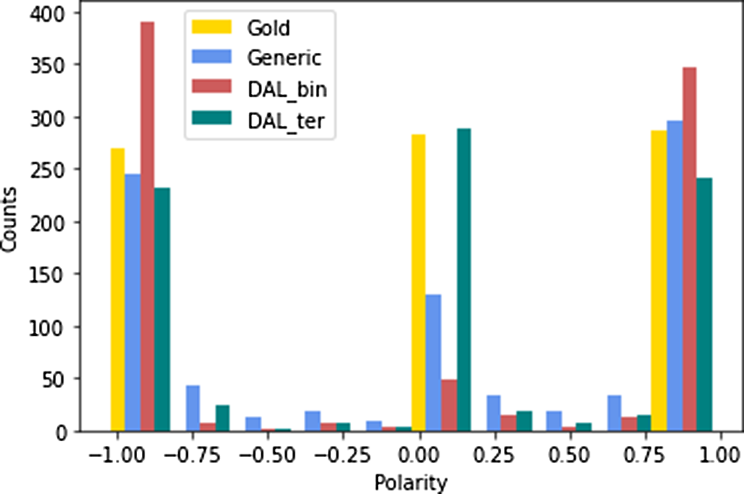
Figure 11. Polarity distribution of different lexicons.
In addition, as no automatic domain adaptation method can avoid introducing noise, we wonder how lexicon noise affects the model performance. Figure 12 shows the CV results of the ATLX model with respect to the increasing size of noisy lexicon entries, where the noise is added by flipping the polarity in the gold lexicon to be a random choice between any opposite polarities but the annotated one (e.g., the polarity of good will be changed to be a random choice between neutral or negative). We find that the model is sensitive to lexicon noise as a significant performance decrease is observed since 20% noise level. Interestingly, the model seems capable of ignoring noisy lexical information because when the noise level keeps increasing, the performance remains close to when no lexicon is applied.

Figure 12. Model performance in accuracy by increasing size of noise in lexicon.
Sentiment aspect adaptation
In Table 11, we create three aspect adapted lexicons with different ways of combining the word vector and the aspect vector. First, we can see that all three methods do not make a huge difference in terms of model performance. Secondly, when compared to the baseline (no lexicon applied), there is only a marginal improvement with an exception of $\text{AAL}_{\textrm{concat}}$
that suffers a decrease on the CV sets. Thirdly, when compared to the ATLX model with generic lexicon, none of the three aspect adapted lexicons are able to achieve superior performance. Thus, we can conclude that the aspect adaptation method does not provide the model with extra useful information to make a better prediction.
$\text{AAL}_{\textrm{concat}}$
that suffers a decrease on the CV sets. Thirdly, when compared to the ATLX model with generic lexicon, none of the three aspect adapted lexicons are able to achieve superior performance. Thus, we can conclude that the aspect adaptation method does not provide the model with extra useful information to make a better prediction.
The reason for that is most likely due to the limitation in terms of size and variability of the training data ensembled from the seed words. More importantly, the aspect-specific polarity difference cannot be properly reflected in the ensembled training data. In other words, the idea is to have the classifier to be able to disambiguate aspect-dependent opinion words such as “ cheap price” vs “ cheap design” and “ low price” vs “ low quality.” However, the size of the seed words limits the chance of these important examples to appear in the training data. On the other hand, due to the selected seed words themselves, they are more likely to be homogeneously positive or negative on all aspects, making for the classifier even harder to learn the difference between aspect-dependent opinion words.
On the other hand, this kind of ambiguity is not usually associated with the aspect directly, it is mostly based on the context. For example, consider the case “ black screen” vs “ black macbook”, where “black screen” is indirectly associated with the aspect quality, and “black macbook” is indirectly associated with the aspect design. Thus, it is hard to connect ambiguous opinion words with the aspects directly. For similar examples, consider: “battery lasts long ” vs “takes a long time to load”; “the laptop will burn my lags” vs “ burn 3 dvds.”
4.4 Direct comparison to related works
Since the works described in this paper expand across multiple years and the NLP filed has been evolving extremely fast, here we compare our work directly to related works focusing mainly in the last five years. In these five years, the dominant approach has shifted from LSTM and attention-based approaches to fine-tuning a pre-trained large language model (LLM) such as BERT (Devlin et al. Reference Devlin, Chang, Lee and Toutanova2019). As LLMs are bigger in terms of both pre-training data size and number of parameters compared to previous approaches, the gap between two paradigms is rather large; however, for the same reason, it is not entirely fair to compare.
Table 12 shows the benchmark comparing our proposed methods with other ABSA systems. As shown in the table, our proposed methods rank among the top non-BERT methods. The ATLX model and its variants rank top among the non-BERT methods in the restaurant domain dataset. In terms of the laptop domain detest, although the results are evaluated on different datasets (SemEval 2014 and SemEval 2015), the performance of our proposed model is at the same level as other systems.
Table 12. Comparison between our proposed methods and other ABSA systems in accuracy on the restaurant and laptop domain datasets. All results of the restaurant domain are based on the SemEval 2014 Task 4 restaurant dataset. All results of the laptop domain are based on the SemEval 2014 Task 4 laptop dataset, except the ones marked by *, which are based on the SemEval 2015 Task 12 laptop dataset. The ATLX + DAL $_{\textrm{ter}}$
experiment is the laptop review domain adaptation experiment explained in Section 4.3; thus, no results present for the restaurant domain.
$_{\textrm{ter}}$
experiment is the laptop review domain adaptation experiment explained in Section 4.3; thus, no results present for the restaurant domain.
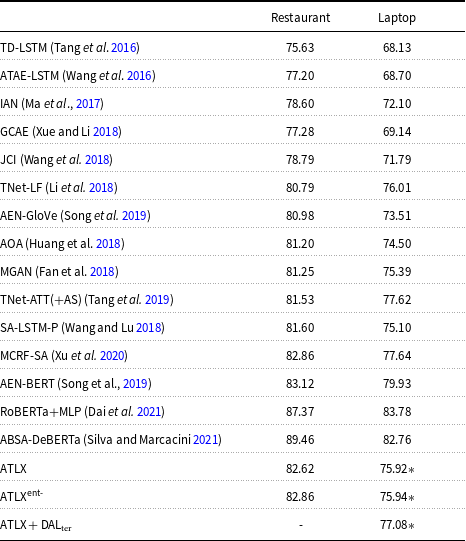
5. Conclusion and future work
In this work, we propose ATLX, a simple yet effective approach to merge the lexical features given by sentiment lexicon with an attention-based LSTM neural network for ABSA. We experiment our approach on two different datasets from different domains and the results prove the effectiveness of our approach.
In addition, we find that the commonly used attention mechanism applied in our experiment is likely to over-fit, especially when applied early in the network for a task such as ABSA. This over-fitting effect hurts the performance by binding the model from key elements for polarity judgment. The effect is shown by comparing the difference between ATLX and the baseline model. Moreover, the effect is also shown when we experiment with two attention regularizers that try to overcome this over-fitting effect. The experimental results show that regularizing the attention vector from being sparse can lead to performance improvement. However, both proposed regularizers are not ideal as the optimum of both regularizers suggests uniformly distributed weights, which is the opposite of what the attention mechanism is able to gain.
Lastly, we try to improve the ATLX system by adapting the generic lexicon to a domain-specific one or even an aspect-specific one. To do that we test the performance gain of sentiment domain adaptation in our system, as most existing researches measure sentiment domain adaptation by recreating an existing domain-specific lexicon. The experimental results suggest that when applied, the improvement from domain adaptation is limited and a good evaluation on lexicon recreation does not necessarily translate to model performance gain.
Perhaps in this paper, the outcomes of the attention regularization experiments are the least expected. As described in Section 4.2.2, in Figure 10, the negative entropy regularizer applied in the baseline system leads to an almost evenly distributed attention vector. However, this kind of distribution does not hurt the model at all, in fact improvements compared to the baseline are generally observed for the negative entropy regularizer (Table 9).
As a fundamental building block of many state of the art models (e.g., Transformer, BERT), the attention framework is designed mimicking the attention of a human being when processing information. In other words, it supposes to discard irrelevant information and “focus” on particular key points. And one would expect having almost evenly distributed attention weights could hurt the model. However, the results in our experiments suggest otherwise. Similarly, the interpretability of attention is questioned in Serrano and Smith (Reference Serrano and Smith2019) as well. In our case, one possible explanation is that, in our model, the attention is applied early in the network, thus filtering more information (i.e., the attention weight distribution being overly sparse) could hurt the performance by passing too little information to deeper layers of the network.
Thus, for future work, one could focus on the relation between the sparsity of the attention distribution and the position that the attention mechanism is applied in the network. In addition, it is also interesting to see whether more recent multi-head attention models such as Transformer (Vaswani et al. Reference Vaswani, Shazeer, Parmar, Uszkoreit, Jones, Gomez, Kaiser and Polosukhin2017) or other network architectures such as BiLSTM could suffer from similar attention over-fitting issues.


 Open access