


Introduction
Paleontologists have studied the dynamics of extinction and origination in the fossil record in great detail, usually with a focus on the magnitude of biodiversity loss or gain (e.g., Newell Reference Newell and Albritton1967; Raup and Sepkoski Reference Raup and Sepkoski1982; Benton Reference Benton1995; Bambach Reference Bambach2006; Alroy Reference Alroy2008). However, the effects of mass extinctions on biotic composition and ecosystem structure do not necessarily scale directly with magnitude, such that magnitude is an incomplete measure of an event's impact on the history of life (Droser et al. Reference Droser, Bottjer, Sheehan and McGhee2000; McGhee et al. Reference McGhee, Sheehan, Bottjer and Droser2004, Reference McGhee, Sheehan, Bottjer and Droser2012; Christie et al. Reference Christie, Holland and Bush2013). Magnitude and effect can be discordant if extinction events vary in selectivity, where selectivity describes variation in extinction magnitude among taxonomic or functional groups or with respect to some parameter, such as body size or geographic range (e.g., Jablonski and Raup Reference Jablonski and Raup1995; Jablonski Reference Jablonski, Jablonski, Erwin and Lipps1996; Kiessling and Aberhan Reference Kiessling and Aberhan2007; Payne and Finnegan Reference Payne and Finnegan2007; Rivadeneira and Marquet Reference Rivadeneira and Marquet2007; Friedman Reference Friedman2009; Harnik Reference Harnik2011; Heim and Peters Reference Heim and Peters2011; Powell and MacGregor Reference Powell and MacGregor2011; Harnik et al. Reference Harnik, Simpson and Payne2012; Vilhena et al. Reference Vilhena, Harris, Bergstrom, Maliska, Ward, Sidor, Strömberg and Wilson2013; Payne et al. Reference Payne, Bush, Heim, Knope and McCauley2016b). Selective events will alter biotic composition, because taxa that experience higher extinction magnitude will decline as a proportion of the surviving biota, while those that experience lower extinction magnitude will increase proportionally (Fig. 1). Extinction and origination will have a greater effect on composition as either magnitude or selectivity increases (Fig. 1) (Payne et al. Reference Payne, Bush, Chang, Heim, Knope and Pruss2016a).
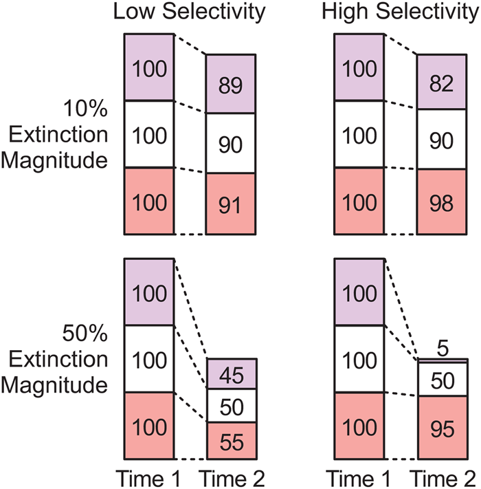
Figure 1. Simple hypothetical example of extinction selectivity with three clades. Numbers indicate species richness before and after an extinction. The combination of high selectivity and high magnitude (bottom right) will lead to large changes in relative taxonomic richness between the clades.
Patterns of extinction selectivity for individual events have received considerable attention, often as a means of evaluating or understanding proposed kill mechanisms (e.g., Kitchell et al. Reference Kitchell, Clark and Gombos1986; Knoll et al. Reference Knoll, Bambach, Canfield and Grotzinger1996, Reference Knoll, Bambach, Payne, Pruss and Fischer2007; Smith and Jeffery Reference Smith and Jeffery1998; Lockwood Reference Lockwood2003; Leighton and Schneider Reference Leighton and Schneider2008; Powell Reference Powell2008; Clapham and Payne Reference Clapham and Payne2011; Alegret et al. Reference Alegret, Thomas and Lohmann2012; Finnegan et al. Reference Finnegan, Heim, Peters and Fischer2012; Clapham Reference Clapham2017; Penn et al. Reference Penn, Deutsch, Payne and Sperling2018). Likewise, selectivity has been evaluated for a number of parameters across broader spans of time, permitting comparisons of mass extinctions with one another and with background intervals (e.g., Payne and Finnegan Reference Payne and Finnegan2007; Janevski and Baumiller Reference Janevski and Baumiller2009; Kiessling and Simpson Reference Kiessling and Simpson2011; Bush and Pruss Reference Bush, Pruss, Bush, Pruss and Payne2013; Payne et al. Reference Payne, Bush, Chang, Heim, Knope and Pruss2016a; Reddin et al. Reference Reddin, Kocsis and Kiessling2019). However, an exact quantitative relationship among magnitude, selectivity, and compositional change has never been derived.
Here, we show that the effects of extinction or origination on biotic composition (C), construed as change in the proportional diversity of a set of clades or functional groups, equals the product of extinction/origination magnitude (M) and selectivity (S) under specific definitions of these parameters. We use this quantitative framework to examine a series of questions about biodiversity dynamics in marine animals: (1) Are mass extinctions more selective than background intervals, and do they drive more taxonomic change? In other words, does the magnitude of an event predict the strength of its effects on biotic composition (cf. Droser et al. Reference Droser, Bottjer, Sheehan and McGhee2000; McGhee et al. Reference McGhee, Sheehan, Bottjer and Droser2004, Reference McGhee, Sheehan, Bottjer and Droser2012; Christie et al. Reference Christie, Holland and Bush2013)? (2) Do mass extinctions form a separate class of events from background intervals with respect to selectivity or effect (cf. Wang Reference Wang2003)? (3) On average, is extinction more selective than origination, and does it drive greater amounts of taxonomic change? (4) Do changes in biotic composition driven by origination during recoveries reverse or reinforce the changes driven by mass extinction? The answers to these questions will help provide a richer view of the ways in which extinction and origination shaped the biosphere through geologic time.
Methods
Extinction
We use the per-stage version of Foote's boundary-crosser metric for extinction magnitude (cf. Foote Reference Foote2003): q = − ln[x bt/(x bt + x bL)], where x bt is the number of taxa crossing the bottom and top boundaries of a time interval and x bL is the number that cross only the bottom boundary (see Table 1 for a listing of abbreviations). The boundary-crosser metric can be standardized by dividing by time-interval duration (Foote Reference Foote1999, Reference Foote2000), which will provide an unbiased estimate of the average magnitude during a time interval (Foote Reference Foote2000). This standardization is beneficial if magnitude is constant or does not vary much within time intervals, whereas the per-stage metric will increase as interval length increases. However, if extinction primarily occurs as pulses within time intervals, as argued by Foote (Reference Foote2005), then the per-stage metric will describe the magnitude of those pulses, whereas the time-standardized metric will vary with interval length (e.g., an extinction pulse would appear half as severe if it were in a time interval twice as long). As we are focused mostly on mass extinctions, we use the per-stage metric, but one could also use the standardized version. Real data undoubtedly reflect a mix of pulsed and background extinction (Stanley Reference Stanley2016), which could potentially be accounted for in future analyses. In our preliminary example presented in the “Results,” we combine some short stages to form longer (and more standardized) time intervals to help ameliorate the potential weaknesses of the per-stage metric.
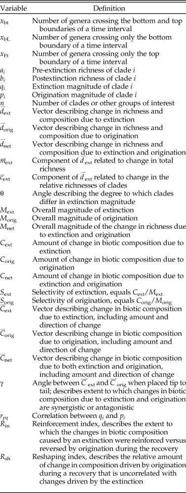
Table 1. Definitions of variables.
The framework derived here also applies to other metrics that treat extinction on a similar scale. In particular, Alroy's gap-filler metric (Alroy Reference Alroy2014, Reference Alroy2015) may be preferable, because it corrects for sampling heterogeneities that may influence the value of q. However, we present the derivation of the method using q, because it is straightforward, and we use q for the preliminary analysis for consistency with the derivation.
Magnitude and Change in Composition
The boundary-crosser metric q can be rewritten as ln(x bt + x bL) − ln(x bt), where x bt + x bL and x bt describe pre- and postextinction richness, considering the set of taxa that enters a time interval. For simplicity, we define a = ln(x bt + x bL) and b = ln(x bt), such that q = a − b. Given n clades or other groups of interest, we define a 1 … a n and b 1 … b n to be the log-transformed pre- and postextinction richnesses of clades 1 through n. Extinction intensities are defined by q 1 … q n, where q i = a i − b i.
In Figure 2A, a and b are plotted for two clades. Total change in the biota is represented by the diagonal vector  ${\mathop{d}^{\vskip -3pt \hskip -4.5pt\rightharpoonup}\! }$ext, which connects the initial composition (black circle) and the final composition (white circle). (Throughout the manuscript, the subscripts “ext” and “orig” will indicate extinction and origination, variables with arrows will denote vectors [e.g., ${\mathop{m}^{\vskip -.5pt \hskip -6pt\rightharpoonup}\!}$], and variables without arrows will denote scalars or lengths of vectors [e.g., m is the length of ${\mathop{m}^{\vskip -.5pt \hskip -6pt\rightharpoonup}\!}$]). The two clades have the same initial richness (a 1 = a 2), but q 1 = 1.0 and q 2 = 2.0, so the first clade fell in richness by a factor of e and the second clade fell by a factor of e 2. The slope of ${\mathop{d}^{\vskip -3pt \hskip -4.5pt\rightharpoonup}\!}}$ext is q 2/q 1 = 2.0; the extent to which this slope differs from 1.0 is one measure of selectivity (variation in extinction intensity among clades). If the vector ${\mathop{d}^{\vskip -3pt \hskip -4.5pt\rightharpoonup}\!}$ext had a different length but the same slope, the ratio of q 2 to q 1 would be the same, meaning that selectivity was constant, although the magnitude of extinction would be different.
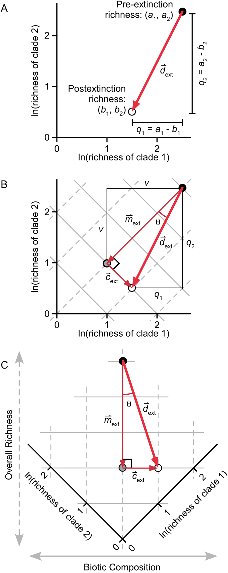
Figure 2. Derivation of metrics for extinction magnitude, selectivity, and change in composition. A, Logged richness values for two hypothetical clades. Vector  ${\mathop{d}^{\vskip -1.5pt \hskip -4.5pt\rightharpoonup}\!\!}$ext represents the overall change in richness and composition of the fauna, and q 1 and q 2 are the boundary-crosser extinction magnitudes for the two clades. B, Same data as in A. The diagonal solid gray lines describe sets of points for which the sum of the logged richness values is constant, and the diagonal dashed gray lines describe sets of points where their difference is constant. Here, ${\mathop{m}^{\vskip -.5pt \hskip -5.5pt\rightharpoonup}\!}$ext is the component of ${\mathop{d}^{\vskip -1.5pt \hskip -4.5pt\rightharpoonup}\!\!}$ext parallel to the dashed gray lines, representing change in total richness, and ${\mathop{c}^{\vskip -.5pt \hskip -4.5pt\rightharpoonup}\!\!}$ext is the component of ${\mathop{d}^{\vskip -1.5pt \hskip -4.5pt\rightharpoonup}\!\!}$ext parallel to the solid gray lines, representing change in the relative richness of the two clades. θ is the angle between ${\mathop{m}^{\vskip -.5pt \hskip -6.5pt\rightharpoonup}\!}$ext and ${\mathop{d}^{\vskip -1.5pt \hskip -4.5pt\rightharpoonup}\!\!}$ext. C, Same as B, rotated 45° counterclockwise so that the horizontal and vertical axes correspond to measures of biotic composition and total richness, respectively.
In Figure 2B, the same data are shown along with solid gray diagonal lines that describe sets of points for which the sum of the logged richness values is constant (e.g., [2,0], [1,1], and [0,2]). For purposes of this derivation, we use this sum as a measure of total diversity. Normally, of course, total diversity would be calculated as the sum of unlogged values, but this is not possible while working in log space, as required for this derivation. We discuss the potential limitations imposed by this approach under “Additional Discussion of Parameters.”
The dashed gray diagonal lines in Figure 2B, whose slopes equal 1.0, describe sets of points for which the difference between the logged richness values of the two clades is constant, indicating that the two clades maintain constant relative richness in arithmetic space. For example, if the difference between two logged richness values is 1.0, then one clade has e times more taxa than the other. The difference in logged richness is a natural measure of biotic composition—that is, the relative taxonomic richnesses of clades.
The diagonal lines in Figure 2B define a set of orthogonal axes that permit one to separate change in total richness from change in relative richness among groups, thus separating the magnitude and compositional effects of an extinction event. In Figure 2C, the diagram from Figure 2B is rotated 45° counterclockwise so that these parameters correspond to the vertical and horizontal axes. In this example, q 1 ≠ q 2, so there are components of change that are parallel to both the dashed and solid gray lines, which are denoted by  ${\mathop{m}^{\vskip -1.5pt \hskip -6.5pt\rightharpoonup}\hskip -1pt}$ext and ${\mathop{c}^{\vskip -.5pt \hskip -4.5pt\rightharpoonup}\!\!}$ext (Fig. 2B,C). Thus, m ext (the length of vector ${\mathop{m}^{\vskip -1.5pt \hskip -6.5pt\rightharpoonup}\hskip -1pt}}$ext) is a measure of the magnitude of the extinction, construed as the change in the sum of the logged richness values of the clades, and c ext (length of ${\mathop{c}^{\vskip -.5pt \hskip -4.5pt\rightharpoonup}\!\!}$ext) is a measure of the amount of compositional change driven by the extinction, construed as change in the relative richnesses of the clades. Although m ext and q i both relate to extinction magnitude, they indicate different aspects: q i describes the extinction magnitude of individual clades, whereas m ext is a measure of total extinction magnitude (Table 1).
To derive a value for m ext, first note that the dot product of two vectors ( ${\mathop{x}^{\vskip -.5pt \hskip -5.5pt\rightharpoonup}\!}$ and ${\mathop{y}^{\vskip -.5pt \hskip -5.5pt\rightharpoonup}\!}$) can be calculated two ways. First, ${\mathop{x}^{\vskip -.5pt \hskip -5.5pt\rightharpoonup}\!}$ · ${\mathop{y}^{\vskip -.5pt \hskip -5.5pt\rightharpoonup}\!}$ equals xycos(θ), where and x and y are the lengths of the vectors and θ is the angle between them. Second, ${\mathop{x}^{\vskip -.5pt \hskip -5.5pt\rightharpoonup}\!}$ · ${\mathop{y}^{\vskip -.5pt \hskip -5.5pt\rightharpoonup}\!}$ equals Σx iyi, where x i and y i are the components of ${\mathop{x}^{\vskip -.5pt \hskip -5.5pt\rightharpoonup}\!}$ and ${\mathop{y}^{\vskip -.5pt \hskip -5.5pt\rightharpoonup}\!}$ in each of the n dimensions (all summations are from i = 1 to i = n, where n is the number of clades and thus dimensions). Thus, xycos(θ) equals Σx iyi. The components of ${\mathop{d}^{\vskip -1.5pt \hskip -4.5pt\rightharpoonup}\!}$ext in the n dimensions are the q i, whereas ${\mathop{m}^{\vskip -1.5pt \hskip -6.5pt\rightharpoonup}\hskip -1pt}}$ext has the same component in each dimension, labeled v in Figure 2B. Replacing ${\mathop{x}^{\vskip -.5pt \hskip -5.5pt\rightharpoonup}\!}$ and ${\mathop{y}^{\vskip -.5pt \hskip -5.5pt\rightharpoonup}\!}$ with ${\mathop{m}^{\vskip -1.5pt \hskip -6.5pt\rightharpoonup}\hskip -1pt}}$ext and ${\mathop{d}^{\vskip -2.5pt \hskip -4.5pt\rightharpoonup}\!\!}$ext gives us m extd extcos(θ) = Σvq i = vΣq i. Cos(θ) can be replaced with m ext/d ext, because ${\mathop{m}^{\vskip -1.5pt \hskip -6.5pt\rightharpoonup}\hskip -1pt}}$ext and ${\mathop{d}^{\vskip -2.5pt \hskip -4.5pt\rightharpoonup}\!\!}$ext form the adjacent side and hypotenuse of a right triangle, which gives us $m_{ext}^2 $ = vΣq i. By the Pythagorean theorem, we know that m ext = $\sqrt {nv^2} $, which rearranges to v = m ext/√n. Replacing v gives us $m_{ext}^2 $ = (m ext/√n)(Σq i), which simplifies to m ext = Σq i/√n.
The amount of change in composition, c ext, is the component of change that is parallel to the solid gray lines, equivalent to the distance between the gray circle and the white circle in Figure 2B,C. The white circle is located at (b 1, b 2), which can also be written as (a 1 − q 1, a 2 − q 2), or as (a 1 − q 1, …, a n − q n) for n taxa. The length of line segment v equals m ext/√n = Σq i/n =  $\bar{q}$, so the coordinates of the gray point are (a 1 − $\bar{q}$, …, a n − $\bar{q}$). The distance between the white and gray circles is then $\sqrt {\mathop \sum \nolimits {\lsqb {\lpar {a_i-\bar{q}} \rpar -\lpar {{a_i}-{q_i}} \rpar } \rsqb }^2} $, or $\sqrt {\mathop \sum \nolimits {\lpar {q_i-\bar{q}} \rpar }^2} $.
Thus, we have shown that for magnitude and change in composition, m ext = Σq i/√n and c ext =  $\sqrt {\mathop \sum \nolimits {\lpar {q_i-\bar{q}} \rpar }^2} $. If we rescale these values by dividing by √n, they become
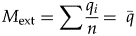 $$M_{{\rm ext}} = \mathop \sum \displaystyle{{q_i} \over n} = \; \bar{q}$$
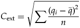 $$C_{{\rm ext}} = \sqrt {\mathop \sum \displaystyle{{{\lpar {q_i-\bar{q}} \rpar }^2} \over n}} $$
where M ext and C ext are the rescaled values of m ext and c ext. Thus, the mean of the extinction magnitudes of the individual clades is a measure of the overall magnitude M ext of the extinction event, and the standard deviation of the extinction intensities (calculated as a population, not a sample) is a measure of the amount of change in composition, C ext. Rescaling by √n means that M ext is measured on the same scale as clade-level extinction magnitude, and it permits direct comparisons when the number of clades varies. C ext is a Euclidean distance between the log-transformed composition of pre- and postextinction biotas, similar to some metrics of dissimilarity among ecological communities (e.g., Faith et al. Reference Faith, Minchin and Belbin1987; Legendre and Legendre Reference Legendre and Legendre2012).
Selectivity
In Figure 2B,C, the angle θ is a measure of the extent to which q 1 ≠ q 2; that is, a measure of selectivity. Rather than using θ itself as the selectivity metric, it is more convenient to use tan(θ), which equals c ext/m ext by definition (Fig. 2B,C). Because C ext and M ext are rescaled by the same factor from c ext and m ext, tan(θ) also equals C ext/M ext. For our purposes, using tan(θ) is effectively equivalent to using θ; the two quantities are monotonically related when 0° < θ < 90°, and they are nearly linearly related when θ < 45°, which should generally be true in real data sets. If q 1 = q 2, θ and tan(θ) are zero (no selectivity), and as the extinction intensities become more dissimilar, θ and tan(θ) increase (selectivity increases).
If we define selectivity of extinction (S ext) to equal tan(θ), then
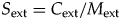 $$S_{{\rm ext}} = C_{{\rm ext}}/M_{{\rm ext}}$$
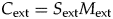 $$C_{{\rm ext}} = S_{{\rm ext}}M_{{\rm ext}}$$
Thus, selectivity is the amount of biotic change divided by extinction magnitude, and, equivalently, the amount of biotic change equals selectivity times magnitude. S ext is the coefficient of variation of the extinction intensities of the individual clades, or the standard deviation divided by the mean. The coefficient of variation is a common way of measuring variation that accounts for differences in the mean; here, selectivity is a measure of the amount of compositional change relative to the overall extinction magnitude. The Supplementary Appendix and Supplementary Figure 1 describe a number of hypothetical extinction scenarios that combine different values of M ext, S ext, and C ext.
Accounting for Time-Interval Duration
As discussed earlier, the boundary-crosser extinction magnitude (as defined here) is sometimes divided by time-interval duration (Δt) in an attempt to correct for variations in duration. Although we do not use this correction here, it is compatible with our metrics for magnitude, selectivity, and change in composition. The mean and standard deviation of (q 1/Δt, …, q i/Δt) equal the mean and standard deviation of (q 1, …, q i) divided by Δt, so M ext/Δt and Cext/Δt are the duration-corrected metrics for magnitude and change in composition. Selectivity (S ext) remains the same, because Δt cancels out when C ext/Δt is divided by M ext/Δt.
Origination and Net Change
Magnitude, selectivity, and change in composition can be calculated for origination simply by replacing extinction intensities with origination intensities in equations (1) and (2), yielding the parameters M orig, S orig, and C orig. Origination intensity for individual clades is calculated as p = −ln[x bt/(x bt + x Ft)] = ln(x bt + x Ft) − ln(x bt), where x bt is number of taxa crossing the bottom and top boundaries of a time interval and x Ft is the number that cross only the top boundary (Foote Reference Foote1999, Reference Foote2000) (Table 1). The derivation follows Figure 2, except that the vector representing diversity change ( ${\mathop{d}^{\vskip -2.5pt \hskip -4.5pt\rightharpoonup}\!\!}$orig) would point to the upper right quadrant instead of the lower left quadrant in Figure 2A,B. An example is shown in rotated view in Figure 3.
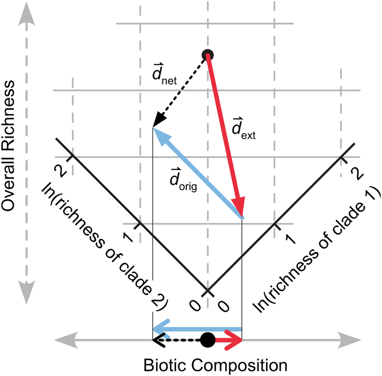
Figure 3. Summing the effects of extinction ( ${\mathop{d}^{\vskip -2.5pt \hskip -4.5pt\rightharpoonup}\!\!}$ext) and origination ( ${\mathop{d}^{\vskip -2.5pt \hskip -4.5pt\rightharpoonup}\!\!}$orig). The logged richness values of two clades are shown, rotated as in Fig. 2C so that the horizontal and vertical axes correspond to biotic composition and overall richness, respectively. Net change ( ${\mathop{d}^{\vskip -2.5pt \hskip -4.5pt\rightharpoonup}\!\!}$net) in diversity is the vector sum of ${\mathop{d}^{\vskip -2.5pt \hskip -4.5pt\rightharpoonup}\!\!}$ext and ${\mathop{d}^{\vskip -2.5pt \hskip -4.5pt\rightharpoonup}\!\!}$orig. The three vectors are projected onto the biotic composition axis at the bottom of the panel.
The net change in the richness of group i due to both extinction and origination is p i − q i = [ln(x bt + x Ft) − ln(x bt)] − [ln(x bt + x bL) − ln(x bt)] = ln(x bt + x Ft) − ln(x bt + x bL), with positive values indicating an increase in total richness and negative values a decrease. Net magnitude of richness change (M net) and net change in composition (C net) can be calculated as the mean and population standard deviation of these negative and positive values. However, we do not define a corresponding selectivity metric, because coefficients of variation are not used for variables that take both positive and negative values. In the analyses presented in the “Results,”  ${\mathop{C}{\vskip -5.5pt\hskip -9pt\rightharpoonup}\!\hskip -1pt}$net is calculated by comparing extinction in one interval and origination in the following interval, an approach that evaluates the total change driven by an extinction and its recovery. One could also calculate ${\mathop{C}{\vskip -5.5pt\hskip -9pt\rightharpoonup}}}$net based on origination and extinction values from the same interval.
C ext, C orig, and C net describe the amount of change in composition, but change in composition also has a direction that describes which clades increase in proportional richness and which decrease. Direction of change is important in understanding how extinction and origination combine to drive biotic change—if the clades that have high extinction magnitude have equivalently high origination magnitude, then the effects of origination and extinction on composition will cancel out. Conversely, if clades that suffer high extinction also suffer low origination, then biotic change will be much more significant. Thus, examining change in composition as vectors is essential to understanding the ultimate effects of extinction and origination.
When plotting the logged richnesses of multiple taxa, the vector representing total diversity change ( ${\mathop{d}^{\vskip -2.5pt \hskip -4.5pt\rightharpoonup}\!\!}$net, black arrow in Fig. 3) is the sum of the vectors representing the changes driven by extinction ( ${\mathop{d}^{\vskip -2.5pt \hskip -4.5pt\rightharpoonup}\!\!}$ext, red arrow) and origination ( ${\mathop{d}^{\vskip -2.5pt \hskip -4.5pt\rightharpoonup}\!\!}$orig, blue arrow). In Figure 3, these three vectors are projected onto the biotic composition axis (bottom), where the black arrow is still the sum of the blue and red. These arrows have lengths of C ext√n, C orig√n, and C net√n; that is, the values for change in composition before rescaling by dividing by √n. With two clades, biotic composition can be described unidimensionally (Fig. 3), and one could use positive and negative numbers to express direction of change.
For n clades, an (n − 1)-dimensional space is needed to represent biotic composition. Thus, the solid gray line representing biotic composition in Figure 3 would expand to a two-dimensional plane for three clades, as shown in Figure 4A. The red, blue, and black vectors represent the change in composition driven by extinction, origination, and their sum ( ${\mathop{C}{\vskip -5.5pt\hskip -9pt\rightharpoonup}}}$ext, ${\mathop{C}{\vskip -5.5pt\hskip -9pt\rightharpoonup}}}$orig, and ${\mathop{C}{\vskip -5.5pt\hskip -9pt\rightharpoonup}}}$net); that is, they are the higher-dimensional analogues of the arrows on the gray axis below Figure 3, rescaled by √n. They represent both the amount of change in composition (their lengths equal C ext, C orig, and C net) and the relative direction of change. Additional clades would increase the dimensionality of this space, but two vectors and their sum always lie in a single plane, so higher-dimensional cases can be represented in two dimensions. For ease of comparison, we always show ${\mathop{C}{\vskip -5.5pt\hskip -9pt\rightharpoonup}}}$ext directed upward with its base at the origin and ${\mathop{C}{\vskip -5.5pt\hskip -9pt\rightharpoonup}}}$orig directed to the right with its base at the tip of ${\mathop{C}{\vskip -5.5pt\hskip -9pt\rightharpoonup}}$ext, as in Figure 4A.
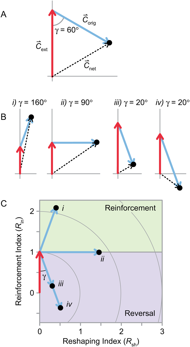
Figure 4. Change in biotic composition for three or more clades. A, Net change in composition ( ${\mathop{C}{\vskip -5.5pt\hskip -9pt\rightharpoonup}}$net) is the vector sum of ${\mathop{C}{\vskip -5.5pt\hskip -9pt\rightharpoonup}}$ext and ${\mathop{C}{\vskip -5.5pt\hskip -9pt\rightharpoonup}}$orig, and γ is the angle between ${\mathop{C}{\vskip -5.5pt\hskip -9pt\rightharpoonup}}$ext and ${\mathop{C}{\vskip -5.5pt\hskip -9pt\rightharpoonup}\!\hskip -1pt}$orig when they are placed tip to tail. B, Various values of ${\mathop{C}{\vskip -5.5pt\hskip -9pt\rightharpoonup}\!\hskip -1pt}$ext, ${\mathop{C}{\vskip -5.5pt\hskip -9pt\rightharpoonup}\!\hskip -1pt}$orig, ${\mathop{C}{\vskip -5.5pt\hskip -9pt\rightharpoonup}\!\hskip -1pt}$net, and γ. When γ is large (i, ii), ${\mathop{C}{\vskip -5.5pt\hskip -9pt\rightharpoonup}\!\hskip -1pt}$net is longer than ${\mathop{C}{\vskip -5.5pt\hskip -9pt\rightharpoonup}\!\hskip -1pt}$ext or ${\mathop{C}{\vskip -5.5pt\hskip -9pt\rightharpoonup}\!\hskip -1pt}$orig (i.e., the effects of extinction and origination on biotic composition are synergistic). When γ is small (iii, iv), ${\mathop{C}{\vskip -5.5pt\hskip -9pt\rightharpoonup}\!\hskip -1pt}$ext and ${\mathop{C}{\vskip -5.5pt\hskip -9pt\rightharpoonup}\!\hskip -1pt}$orig will cancel out to some extent when summed to form ${\mathop{C}{\vskip -5.5pt\hskip -9pt\rightharpoonup}\!\hskip -1pt}$net. C, The sets of vectors from B are rescaled so that ${\mathop{C}{\vskip -5.5pt\hskip -9pt\rightharpoonup}\!\hskip -1pt}$ext has unit length. ${\mathop{C}{\vskip -5.5pt\hskip -9pt\rightharpoonup}\!\hskip -1pt}$net vectors have been excluded for clarity; however, the values of C net relative to C ext are described by the circles, with values indicated on the vertical axis. The reinforcement index (R in) and reshaping index (R sh) correspond to the vertical and horizontal axes, respectively.
With three or more taxa,  ${\mathop{C}{\vskip -5.5pt\hskip -9pt\rightharpoonup}\!\hskip -1pt}$ext and ${\mathop{C}{\vskip -5.5pt\hskip -9pt\rightharpoonup}\!\hskip -1pt}$orig can form any angle from 0° to 180°, denoted here as γ (Fig. 4A). If γ is large, ${\mathop{C}{\vskip -5.5pt\hskip -9pt\rightharpoonup}\!\hskip -1pt}$net will be longer than either ${\mathop{C}{\vskip -5.5pt\hskip -9pt\rightharpoonup}\!\hskip -1pt}$ext or ${\mathop{C}{\vskip -5.5pt\hskip -9pt\rightharpoonup}\!\hskip -1pt}$orig (Fig. 4B, scenarios i and ii). If γ is small, however, ${\mathop{C}{\vskip -5.5pt\hskip -9pt\rightharpoonup}\!\hskip -1pt}$ext and ${\mathop{C}{\vskip -5.5pt\hskip -9pt\rightharpoonup}\!\hskip -1pt}$orig will to some extent cancel out, and ${\mathop{C}{\vskip -5.5pt\hskip -9pt\rightharpoonup}\!\hskip -1pt}$net, their sum, will be shorter than either or both of them (Fig. 4B, scenarios iii and iv). Given the right combination of angle and vector lengths, ${\mathop{C}{\vskip -5.5pt\hskip -9pt\rightharpoonup}\!\hskip -1pt}$net could have the same length as either ${\mathop{C}{\vskip -5.5pt\hskip -9pt\rightharpoonup}\!\hskip -1pt}$orig and ${\mathop{C}{\vskip -5.5pt\hskip -9pt\rightharpoonup}\!\hskip -1pt}$ext or both (Fig. 4A). The angle γ can be calculated from the correlation coefficient between the clade-level origination and extinction magnitudes (r pq):
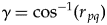 $$\gamma = {\rm co}{\rm s}^{-1}\lpar {r_{\,pq}} \rpar $$
The derivation for equation (5) is shown in the Appendix, as are the derivations for the following equations for calculating C net, which might be convenient in some cases:
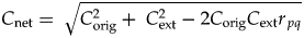 $$C_{{\rm net}} = \; \sqrt {C_{{\rm orig}}^2 + \; C_{{\rm ext}}^2 -2C_{{\rm orig}}C_{{\rm ext}}r_{\,pq}} \; \; $$
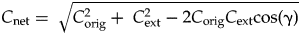 $$C_{{\rm net}} = \; \sqrt {C_{{\rm orig}}^2 + \; C_{{\rm ext}}^2 -2C_{{\rm orig}}C_{{\rm ext}}{\rm cos}\lpar {\rm \gamma} \rpar } \; \; $$
 In the analyses presented in the “Results,”  ${\mathop{C}{\vskip -5.5pt\hskip -9pt\rightharpoonup}\!\hskip -1pt}$net is calculated by comparing extinction in one interval with origination in the following interval, an approach that evaluates the total change driven by an extinction and its recovery. In this case, γ describes the degree to which extinctions and recoveries have similar or opposite effects on biotic composition.
Reinforcement, Reversal, and Reshaping of Biotic Change
We define two additional parameters, the reinforcement index (R in) and the reshaping index (R sh):
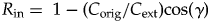 $$R_{{\rm in}} = \; 1{\rm} -{\rm} \lpar {C_{{\rm orig}}/C_{{\rm ext}}} \rpar {\rm} {\rm cos}\lpar \gamma \rpar $$
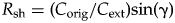 $$R_{{\rm sh}} = \lpar {C_{{\rm orig}}/C_{{\rm ext}}} \rpar {\rm} {\rm sin}\lpar {\rm \gamma} \rpar $$
In Figure 4C, each set of vectors from Figure 4B is rescaled so that C ext = 1, which means that R in is displayed on the vertical axis and R sh is displayed on the horizontal axis.
The reinforcement index describes the extent to which the changes in biotic composition caused by extinction were reinforced versus reversed by origination during the recovery (i.e., it is the component of  ${\mathop{C}{\vskip -5.5pt\hskip -9pt\rightharpoonup}\!\hskip -1pt}$orig that is parallel to ${\mathop{C}{\vskip -5.5pt\hskip -9pt\rightharpoonup}\!\hskip -1pt}$ext; Fig. 4C). For example, if a mass extinction caused the proportion of mollusks to rise relative to the proportion of brachiopods (i.e., the mollusk extinction magnitude was lower), then R in > 1 would indicate that mollusks also gained relative to brachiopods during the recovery (i.e., the mollusk origination magnitude was higher, and γ > 90°; example i in Fig. 4B,C). If R in = 1, then the two clades did not change in relative richness during the recovery (γ = 90°; scenario ii in Fig. 4B,C). R in < 1 would indicate that brachiopods increased at the expense of mollusks during the recovery, at least partially reversing the effects of the extinction (γ < 90°; scenario iii in Fig. 4B,C). R in = 0.0 indicates that all changes were reversed, and R in < 0.0 means that the recovery reversed all changes and caused the fauna to change in the opposite way (e.g., brachiopods recovered so strongly that they ended up relatively more diverse than they were in the pre-extinction fauna; scenario iv in Fig. 4B,C). R in is scaled relative to C ext, so R in = 2.0 means that the recovery doubled the change caused by extinction.
The reshaping index describes the amount of change in composition driven by origination that is uncorrelated with the change driven by extinction (i.e., the component of  ${\mathop{C}{\vskip -5.5pt\hskip -9pt\rightharpoonup}\!\hskip -1pt}$orig perpendicular to ${\mathop{C}{\vskip -5.5pt\hskip -9pt\rightharpoonup}\!\hskip -1pt}$ext; Fig. 4C). If, as described earlier, mollusks gained relative to brachiopods as a result of extinction, then reshaping during the recovery could include echinoderms gaining at the expense of cnidarians, or any other change that did not involve mollusks relative to brachiopods. Like R in, R sh is scaled relative to C ext; R sh = 1.0 indicates that reshaping accomplished as much biotic change as the extinction itself.
Error Bars
To account for uncertainty in values of magnitude, selectivity, and change in composition due to random sampling error, we calculated errors bars around our parameter estimates using Bayesian 95% credible intervals (see Supplementary Appendix for R code). Each of the three parameter estimates is based on the extinction magnitudes of the clades in a given interval (the q i). These extinction magnitudes are subject to binomial random variability, and this variability must be accounted for in the error bars. Calculating frequentist confidence intervals in this situation is not straightforward, because selectivity and change in composition are complicated functions of the extinction magnitudes. We therefore used a Bayesian simulation-based approach. For each clade in each time interval, we used a standard Bayesian model for estimating the binomial probability of a genus going extinct (Wang Reference Wang, Alroy and Hunt2010). We used a uniform distribution as the prior, combining it with fossil occurrence data to generate a posterior distribution for the probability of extinction. We then randomly sampled 1000 values from this posterior distribution, which we used to estimate the posteriors for the q i (or p i) in each time interval. Using the posteriors for all q i in a time interval, we derived the posterior distributions of magnitude, selectivity, and change in composition for that interval. We then took the middle 95% of each posterior, giving us 95% equal-tail credible intervals. These credible intervals are analogous to frequentist confidence intervals and quantify the uncertainty in the estimated values of magnitude, selectivity, and change in composition, accounting for variability due to clade size and uncertainty in the underlying extinction rates.
Additional Discussion of Parameters
Magnitude
Our metrics for extinction and origination magnitude give each clade equal weight, regardless of individual richness. In contrast, the overall extinction or origination intensity for a biota is typically calculated by lumping all taxa into a single pool, such that more diverse clades more strongly influence the value. If one considers clades to be the units of interest in the analysis, then giving clades equal weight is legitimate. In any case, for the example presented on marine animals (see “Results”), M ext and M orig are highly correlated with magnitude calculated by pooling all taxa (r 2 ≥ 0.95 with p << 0.01 for raw data and first differences), suggesting that this difference in approach will not present practical difficulties in many cases. Excluding clades with very low richness (see “Small Sample Sizes”) should also strengthen this correspondence. However, the correlation between M and q or p based on the pooled fauna would be weaker if clades differed greatly in both richness and extinction/origination magnitude. In that case, the methods outlined here may not be well suited to the data.
Change in Composition
Change in composition is calculated as a Euclidean distance based on a measure of the relative number of species or genera within clades, much like how one might calculate dissimilarity among communities or fossil assemblages using the relative number of individuals within species (e.g., Faith et al. Reference Faith, Minchin and Belbin1987; Legendre and Legendre Reference Legendre and Legendre2012). Thus, our C metrics have straightforward, intuitive interpretations. To further satisfy ourselves that our C ext and C orig are reasonable, we compared values calculated from the marine animal data set (see “Results”) with values of Bray-Curtis dissimilarity calculated on proportional logged richness data for pre- and postextinction faunas and pre- and postorigination faunas. For raw data and first differences for both C ext and C orig, r 2 ≥ 0.92 with p << 0.01. The two metrics are calculated quite differently (Bray-Curtis is nonmetric and non-Euclidean), but we present the comparison simply to show that C captures the same basic information as a metric that is commonly used in studies of ecological and paleoecological gradients (Clarke and Warwick Reference Clarke and Warwick2001; Bush and Brame Reference Bush and Brame2010; Legendre and Legendre Reference Legendre and Legendre2012) and in studies of faunal change through time (Clapham Reference Clapham2015).
Small Sample Sizes
It may be difficult to interpret M, C, and S when some clades have very low richness, because stochastic variations could lead to greatly different parameter estimates. At the extreme, a clade that only has one genus will have an observed extinction intensity of either zero or infinity, regardless of the underlying probability of extinction. Credible intervals, as implemented here, should help in the interpretation of parameter values based on low-richness clades by highlighting the high uncertainty associated with such values. In the analysis presented in the “Results,” we also excluded individual clades from time intervals in which richness was extremely low (x bt + x bL < 8 genera for extinction; x bt + x Ft < 8 genera for origination).
Low Magnitude
Quantification of selectivity will be inherently uncertain when extinction/origination magnitude is very low. S ext and S orig are equivalent to coefficients of variation, which become sensitive to small changes in the denominator (M ext or M orig) as it approaches zero (cf. Gould Reference Gould1984). Thus, selectivity could take on anomalously high and/or uncertain values when magnitude is extremely low. To the extent that variations in extinction/origination intensity among groups are driven by random sampling error, credible intervals like those used here will assist in quantifying this uncertainly (e.g., selectivity is high, but the credible interval extends to low values). However, it is likely that some variation in extinction/origination intensity among groups is driven by other types of heterogeneity in the data, such as variations in sampling and preservation, which may not be captured by our methodology and which are more difficult to model. Difficulty in precisely quantifying selectivity when magnitude is low is a problem for other selectivity metrics as well, because no technique will accurately quantify variation among variables whose values are so small that errors overwhelm the signal.
Infinite Values
When a clade goes completely extinct, the calculated extinction intensity equals infinity with the boundary-crosser metric, and M ext and C ext will also equal infinity (likewise for origination at a clade's earliest appearance). Infinite values are inherently awkward to evaluate, and they are misleading in many cases. To the extent that calculated extinction intensity is an estimate of the underlying probability that individual taxa in a clade go extinct, boundary-crosser values of infinity imply that all members of a clade are absolutely guaranteed to die. In reality, the underlying probability is probably less than 100%, corresponding to a high but not infinite boundary-crosser value. The sample analysis presented in the “Results” was conducted at the phylum level, so no group ever went completely extinct and infinite magnitudes were not an issue.
If infinite values do occur in an analysis, several measures could be taken. Excluding clades from time intervals in which they have few genera, as discussed earlier, should help, because infinite values may be most common in these cases. In addition, our Bayesian credible interval routine provides finite error bars even when all component taxa in a group go extinct. To get point estimates for M and C, one could use the mean or median of the posterior distribution for each parameter.
Comparisons with Other Methods
Used individually, M and C should generally produce results that are similar to existing metrics, as seen earlier. This is not unexpected, as reasonable methods that measure the same phenomenon should produce broadly similar results. The primary benefits of the framework described here are that magnitude, selectivity, and change in composition are measured on compatible scales, and clear relationships among them are derived from first principles. Also, the framework permits the development of new kinds of metrics, such as R in and R sh, that can be applied to macroevolutionary questions. The parameters are simple to calculate once clade-level values for extinction/origination have been determined (eqs. 1, 2).
Our selectivity metric, S, describes variation in extinction magnitude among a set of groups. Multiple logistic regression, which is commonly used in selectivity studies, can measure selectivity with respect to other types of variables, such as binary traits (e.g., benthic vs. pelagic) or continuous traits (e.g., body size). It can also evaluate multiple predictors at once. Thus, the two methods are useful in different circumstances. Payne et al. (Reference Payne, Bush, Chang, Heim, Knope and Pruss2016a) calculated the “influence” of an extinction event on a biota as the geometric mean of selectivity (logistic regression coefficient) and magnitude (percent loss), which is somewhat similar to the relationship we derive here. However, they did not provide a detailed justification for combining these parameters.
Alroy (Reference Alroy2000, Reference Alroy2004) also developed a set of methods that are similar in some respects to the one presented here. The “proportional volatility index” measures change in taxonomic composition, similar to our C metrics, although calculated differently (Alroy Reference Alroy2000). The “proportional volatility G statistic” quantifies the extent to which observed intensities of extinction and/or origination for taxa within a particular time interval differ from those expected given the average value for each group among time intervals and the overall intensity within the interval of interest (Alroy Reference Alroy2000, Reference Alroy2004). Both metrics were applied to overall changes in composition between adjacent time intervals, although they could be split into contributions from extinction and origination.
Like our selectivity metric, the G statistic measures variation in turnover among groups, but the methods are different in important ways. The G statistic quantifies the extent to which the extinction magnitudes of taxa in a particular time interval differ from their expected values given long-term averages. In contrast, S ext simply measures variation in extinction magnitude among taxa within a time interval, standardized by overall magnitude, without comparison to long-term average values. Thus, the metrics are designed to answer different questions. For the questions that we are investigating, our methods have the added benefit that S, C, and M are related (eqs. 3, 4).
Data
We applied these methods to the Phanerozoic marine animal fossil record, which has been the subject of extensive work on extinction and origination magnitude (e.g., Raup and Sepkoski Reference Raup and Sepkoski1982; Bambach et al. Reference Bambach, Knoll and Wang2004; Foote Reference Foote2005, Reference Foote2007; Stanley Reference Stanley2007; Alroy Reference Alroy2008) and some on selectivity (Payne and Finnegan Reference Payne and Finnegan2007; Kiessling and Simpson Reference Kiessling and Simpson2011; Bush and Pruss Reference Bush, Pruss, Bush, Pruss and Payne2013; Payne et al. Reference Payne, Bush, Chang, Heim, Knope and Pruss2016a). For this initial trial, we analyzed an updated version of Sepkoski's (Reference Sepkoski2002) compendium (Heim et al. Reference Heim, Knope, Schaal, Wang and Payne2015). Phanerozoic-scale patterns of origination and extinction are generally similar in the Paleobiology Database (Alroy Reference Alroy2014). We included six diverse phyla that provide mostly continuous series of extinction intensities spanning most of the Phanerozoic at the stage level: Arthropoda, Brachiopoda, Chordata, Cnidaria, Echinodermata, and Mollusca.
We combined consecutive stages in several cases in which stage length and/or number of extinctions was low. We excluded the Cambrian and Tremadocian (earliest Ordovician), because more than one phylum was below our sample-size cutoff of eight genera for x bt + x bL and/or x bt + x Ft. This cutoff is somewhat arbitrary, but it allows us to include at least five phyla for all time intervals. The Cnidaria were excluded from the analysis for several time intervals in which they did not meet this cutoff (Floian/Dapingian, Lopingian, Early Triassic, Anisian). Values of M, S, and C were highly similar when based on five versus six phyla for time intervals that met the sample-size cutoff (r 2 between 0.90 and 0.98).
Of the 56 time intervals in the analysis, we highlight 13 that encompass the “big five” mass extinctions of Raup and Sepkoski (Reference Raup and Sepkoski1982), the Early Triassic, and most of the minor mass extinctions listed by Bambach (Reference Bambach2006) (excluding the Pliensbachian–Toarcian event, which did not clearly stand out in the analysis). For analyses of origination, we highlighted the time intervals that followed these 13, because elevated origination followed many mass extinctions (e.g., Stanley Reference Stanley2007; Alroy Reference Alroy2008; Foote Reference Foote, Bell, Futuyma, Eanes and Levinton2010). Table 2 lists the specific time intervals used to characterize each event.
Table 2. Extinction events and recovery intervals highlighted in the analysis. The big five mass extinctions of Raup and Sepkoski (Reference Raup and Sepkoski1982) are marked in bold.
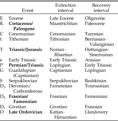
As noted earlier, C net, γ, R in, and R sh were calculated based on C ext in one interval and C orig in the following interval, an approach that evaluates the total change driven by an extinction event and by origination during the subsequent recovery. For these parameters, the Cnidaria had to be excluded from an additional time interval (Capitanian), because the subsequent interval (Lopingian) did not meet the sample-size cutoff.
Results
Extinction
The Ordovician through Neogene history of extinction magnitude M ext (Fig. 5A), which is the average of the clade-level values of q, was similar to the results of previous analyses of marine fossil animals (e.g., Alroy Reference Alroy2008, Reference Alroy2014) (see Supplementary Tables 1–3 for raw results of analyses). Mass extinctions, construed as either the big five or as all events listed in Table 2, were not significantly different in selectivity S ext from background intervals, at least in this preliminary phylum-level analysis (p > 0.05, Mann-Whitney U-test) (Figs. 5B and 6C, Table 3). The Late Ordovician mass extinction and the Givetian had low selectivity, the Early Triassic had extremely high selectivity, and all other mass extinctions were fairly similar (Fig. 5B). A number of background intervals had high selectivity (>0.75) and low magnitude (Fig. 5D), but M ext and S ext were not correlated (r 2 = 0.03, p > 0.05).
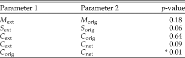
Table 3. The p-values from statistical tests of single parameters. The first two columns report p-values from two-sided Mann-Whitney U-test comparisons of mass extinctions and all other time intervals, with mass extinctions encompassing either the big five events of Raup and Sepkoski (Reference Raup and Sepkoski1982) or all events (“All MEs”) listed in Table 2. The final two columns report p-values from Silverman's critical bandwidth test for multimodality. Double asterisks (**) mark p-values less than 0.01, and single asterisks (*) mark p-values less than 0.05.
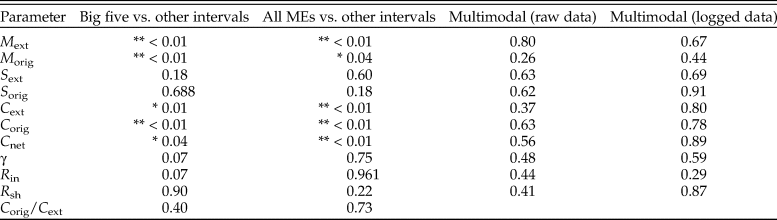
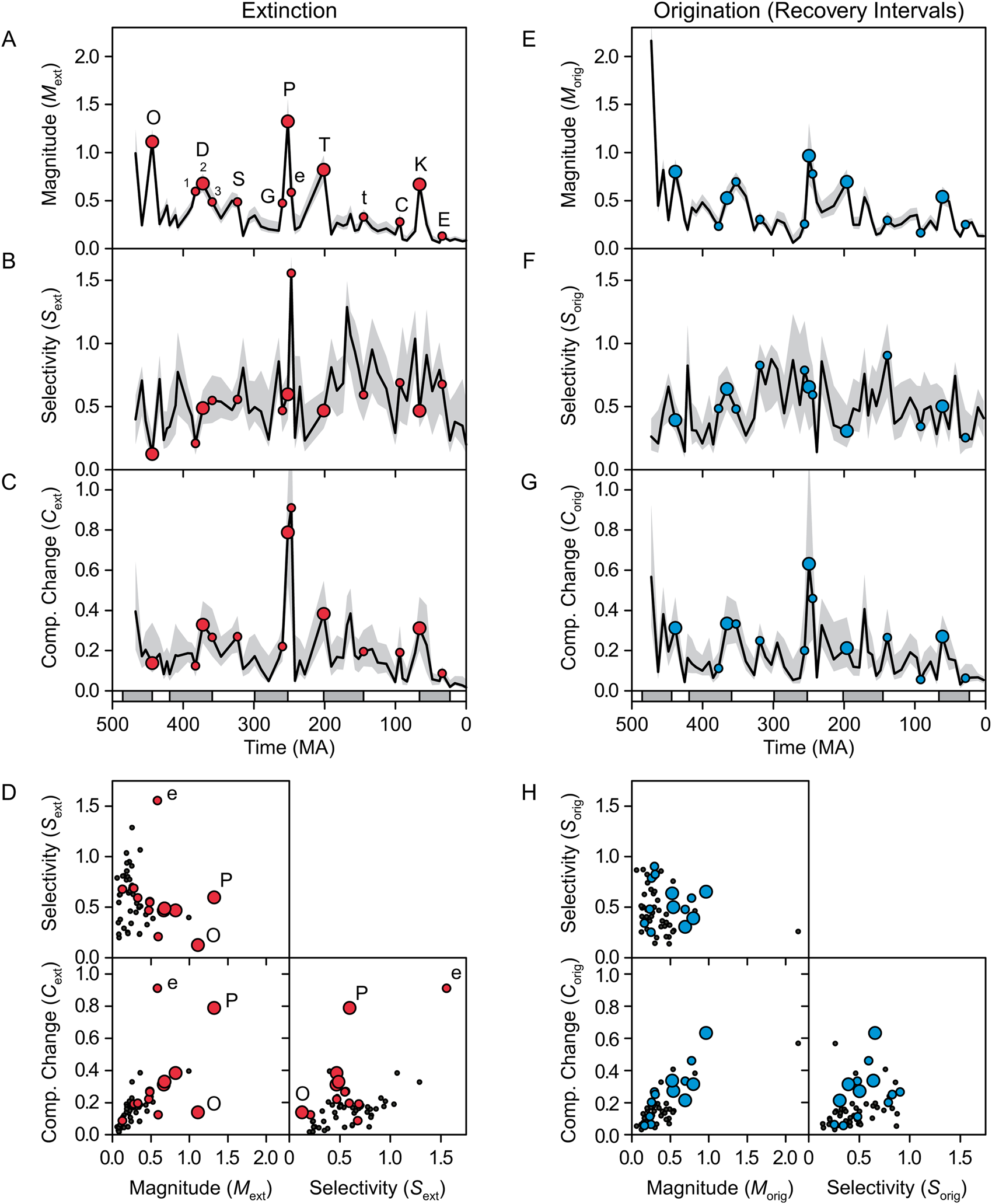
Figure 5. Magnitude, selectivity, and the resulting change in biotic composition (“Comp. Change”) for extinction (A–D) and origination (E–H) in marine animals. The gray bands show 95% credible intervals. For extinction (A–D), the larger circles mark the big five mass extinctions, and the smaller circles mark minor extinction events. For origination (E–H), the circles mark recovery intervals (i.e., the time intervals following the extinctions). Points are plotted at the ends of time intervals for extinction and at their midpoints for origination. The highlighted extinction intervals are labeled in A: O, Late Ordovician; D1, Givetian; D2, Frasnian/Famennian; D3, Devonian/Carboniferous; S, Serpukhovian; G, Guadalupian; P, Permian/Triassic; e, Early Triassic; T, Triassic/Jurassic; t, Tithonian; C, Cenomanian; K, Cretaceous/Paleogene; E, Eocene.
By far, extinction forced the greatest change in composition during the end-Permian event and the Early Triassic (Fig. 5C), with the other mass extinctions causing, at most, half as much change. Change in composition was significantly greater for mass extinctions than for other intervals (Table 3, Fig. 6E), and M ext and C ext were correlated more strongly than S ext and C ext (r 2 = 0.45 vs. 0.24, p << 0.01 for both; Fig. 5D). Given its extremely low selectivity, the Late Ordovician extinction caused little change in composition for its magnitude, whereas highly selective extinction in the Early Triassic caused an unusually large amount of change (after removing these two intervals, r 2 between M ext and C ext rose to 0.73).
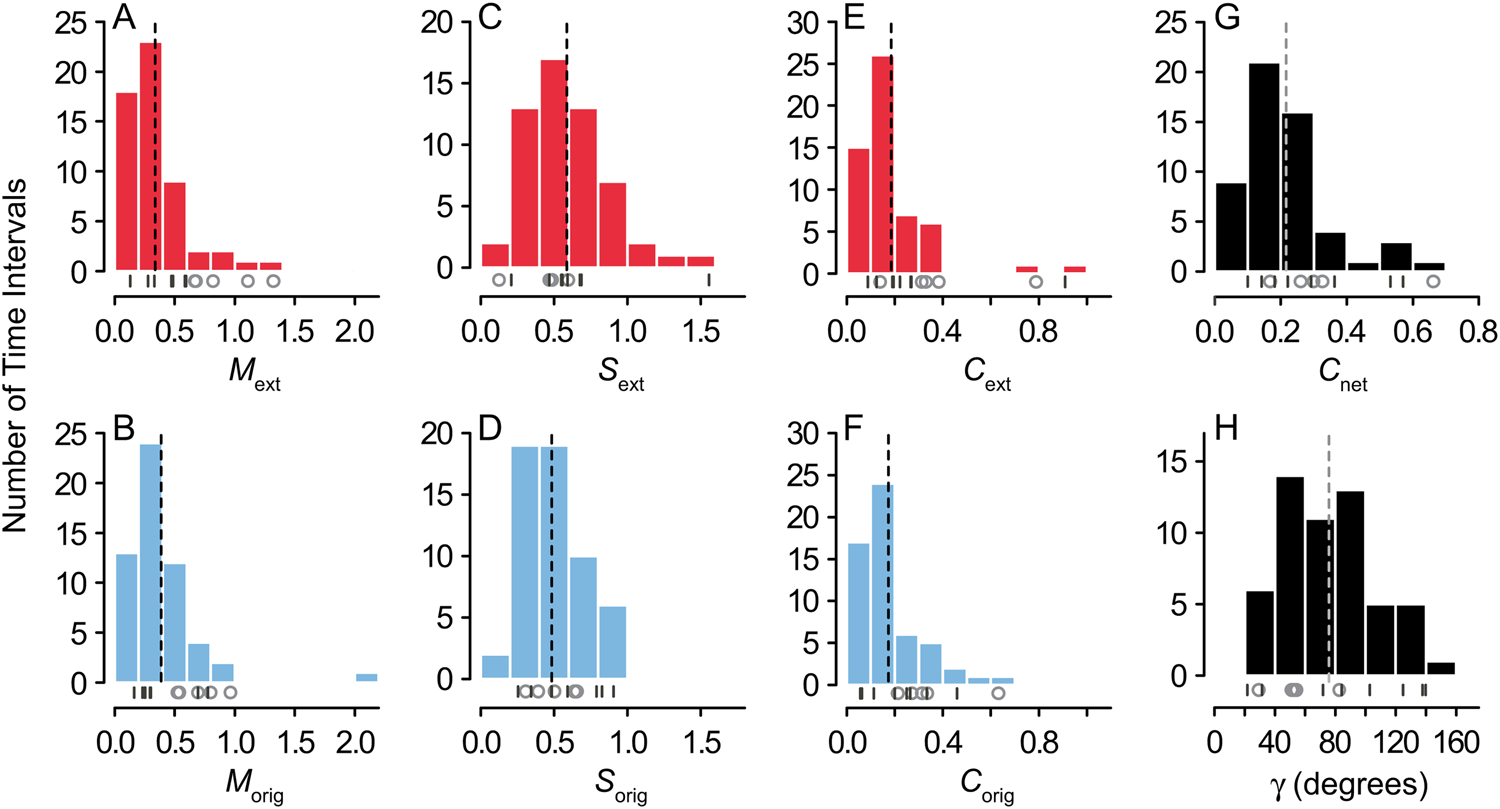
Figure 6. Histograms of extinction and origination magnitude (A,B), selectivity (C,D), and change in composition (E,F); total change in composition (G); and the angle γ between the vectors  ${\mathop{C}{\vskip -5.5pt\hskip -9pt\rightharpoonup}\!\hskip -1pt}$ext and ${\mathop{C}{\vskip -5.5pt\hskip -9pt\rightharpoonup}\!\hskip -1pt}$orig (H). Dashed vertical lines mark mean values. Beneath the histograms, open circles mark the values of the big five mass extinctions, and dashes mark the positions of the minor mass extinctions listed in Table 2.
Origination
Overall, origination magnitude and change in composition were elevated during recovery intervals (cf. Alroy Reference Alroy2008; Foote Reference Foote, Bell, Futuyma, Eanes and Levinton2010), although selectivity was not (Table 3, Figs. 5E–G and 6B,D,F; note that origination is highlighted for time intervals immediately following extinctions). In fact, C orig was significantly correlated with C ext from the previous time interval (r 2 = 0.45 for raw data and 0.23 for first differences, p << 0.01 for both). The recoveries that followed the end-Permian extinction and the Early Triassic had high magnitude of origination and reasonably high selectivity, and as a result, they drove more change in composition than the other recoveries (Fig. 5E–G). Origination magnitude and change in composition were also high for the first interval in the time series (Floian/Dapingian), representing the continuing Ordovician radiation (Fig. 5E,G). As was the case for extinction, change in composition was more strongly correlated with magnitude than with selectivity (r 2 = 0.59 with p << 0.01 vs. r 2 = 0.12 with p = 0.01; Fig. 5H). Overall, values of M, S, and C did not significantly differ between extinction and origination (Fig. 6A–F, Table 4).
Table 4. Results of two-sided Mann-Whitney U-test comparisons of two parameters. Single asterisks (*) mark p-values less than 0.05.
Net Change
C net (change in composition driven by extinction plus origination in the following time interval) was significantly different for mass extinctions than for other intervals (Table 3, Fig. 6G). Overall, C net was not significantly greater than C ext, although it was significantly (though only slightly) greater than C orig (Table 4, Fig. 6E–G). C net was higher than C ext for some extinctions (e.g., Ordovician, Famennian, and Eocene extinctions) and lower for others (e.g., Permian, Triassic, and Cretaceous extinctions; Early Triassic) (Fig. 7A). The vector representations of  ${\mathop{C}{\vskip -5.5pt\hskip -9pt\rightharpoonup}\!\hskip -1pt}$ext, ${\mathop{C}{\vskip -5.5pt\hskip -9pt\rightharpoonup}\!\hskip -1pt}$orig, and ${\mathop{C}{\vskip -5.5pt\hskip -9pt\rightharpoonup}\!\hskip -1pt}$net show how the former case is associated with a large angle (γ) between ${\mathop{C}{\vskip -5.5pt\hskip -9pt\rightharpoonup}\!\hskip -1pt}$ext and ${\mathop{C}{\vskip -5.5pt\hskip -9pt\rightharpoonup}\!\hskip -1pt}$orig, whereas the latter is associated with a small angle (Fig. 7B). This angle did not differ significantly between mass extinctions and background intervals (Table 3, Fig. 6H). The observed values of γ were also no different from those obtained by randomly pairing sets of q i and p i from different time intervals or from random pairing among the 13 mass extinctions and recoveries listed in Table 2 (Mann-Whitney U-test, p > 0.05).
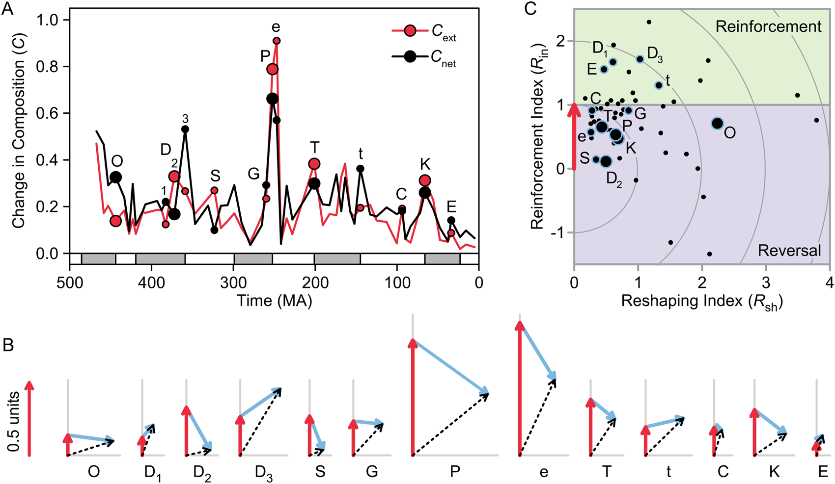
Figure 7. Net change in biotic composition calculated with a one-interval lag between extinction and origination. A, Comparison of net change (C net) and change driven by extinction (C ext). B, Vector representations of the change in composition driven by extinction ( ${\mathop{C}{\vskip -5.5pt\hskip -9pt\rightharpoonup}}\!\hskip -1pt}$ext, red), origination ( ${\mathop{C}{\vskip -5.5pt\hskip -9pt\rightharpoonup}}\!\hskip -1pt}$orig, blue), and their sum ( ${\mathop{C}{\vskip -5.5pt\hskip -9pt\rightharpoonup}}\!\hskip -1pt}$net, black), oriented so that ${\mathop{C}{\vskip -5.5pt\hskip -9pt\rightharpoonup}}\!\hskip -1pt}$ext points up. ${\mathop{C}{\vskip -5.5pt\hskip -9pt\rightharpoonup}}\!\hskip -1pt}$ext was highest during the late Permian and Early Triassic due to high extinction magnitude in the former and high selectivity in the latter (Fig. 5A–C). C, Reinforcement and reshaping indices (R in and R sh). In A and C, large circles mark the big five mass extinctions, and small circles mark minor mass extinctions. O, Late Ordovician; D1, Givetian; D2, Frasnian/Famennian; D3, Devonian/Carboniferous; S, Serpukhovian; G, Guadalupian; P, Permian/Triassic; e, Early Triassic; T, Triassic/Jurassic; t, Tithonian; C, Cenomanian; K, Cretaceous/Paleogene; E, Eocene.
Reinforcement, Reversal, and Reshaping
In Figure 7C, the reinforcement and reshaping indices (R in and R sh) for all time intervals are plotted as in Figure 4C, but with the blue arrows removed for clarity. The recoveries from the big five mass extinctions are all characterized by partial reversal (0 < R in < 1); that is, some of the change in biotic composition driven by extinction was reversed by origination during the recovery. In the case of the Frasnian extinction (D2), almost all of the change was reversed (R in near zero). R in describes the amount of change during a recovery relative to the value of C ext, not the absolute magnitude of change, which is shown in Figure 7B. Thus, mass extinctions and recoveries accomplished large amounts of total change (C net) despite this tendency toward reversal.
Reinforcement occurred during the recoveries from several of the minor extinctions (Givetian, Famennian, Tithonian, and Eocene). Background intervals (black dots) were not significantly different from mass extinctions on either axis (Mann-Whitney U-test; Table 3), reflecting the fact that mass extinctions and background intervals did not differ significantly in γ or C orig/C ext (Table 3).
The average value of R in was 0.76, with a bootstrapped 95% confidence interval of (0.59, 0.93) (bootstrapping based on 10,000 iterations). In other words, the mean of R in was significantly different from 1.0, indicating a tendency toward some reversal of biotic change driven by extinction. However, for the big five events, the average R in was lower, with a mean of 0.49 and a 95% confidence interval of (0.29, 0.65). The average amount of reshaping was 0.98, with a 95% confidence interval of (0.79, 1.19). There was an unusually large amount of reshaping during the recovery from the Late Ordovician extinction (Fig. 7C).
Discussion
General Patterns
Mass Extinctions versus Background Intervals
On average, mass extinctions and their recoveries drove more biotic change than background intervals, a result that holds when Raup and Sepkoski's (Reference Raup and Sepkoski1982) big five events are compared with other intervals or when all highlighted intervals in Table 2 are compared with other intervals (Figs. 5, 6, Table 3). However, there is considerable overlap in C ext and in C orig between mass extinctions and other intervals due to low selectivity of some mass extinctions (e.g., Late Ordovician and Givetian; Fig. 5A–C) and the inclusion of extinction events that represent local maxima in M ext during times of low background values, particularly during the Mesozoic and Cenozoic (Fig. 5A). Some events in this latter group, particularly the Cenomanian and Eocene, also show up as local maxima in C ext (Fig. 5C).
Mass extinctions and their recoveries did not differ significantly from background intervals in selectivity, and change in composition C ext was correlated more strongly with magnitude M ext than selectivity S ext (Fig. 5D). Thus, overall, major extinction events drove larger-than-normal changes in biotic composition, primarily due to greater magnitude. This result seemingly contrasts with demonstrations that mass extinction magnitude and ecological effects are not strongly related (Droser et al. Reference Droser, Bottjer, Sheehan and McGhee2000; McGhee et al. Reference McGhee, Sheehan, Bottjer and Droser2004, Reference McGhee, Sheehan, Bottjer and Droser2012; Christie et al. Reference Christie, Holland and Bush2013), possibly implying that taxonomic and ecological effects have different relationships with magnitude. However, the correlation between magnitude and ecological effects would be more apparent if background time intervals were included in the comparisons of McGhee et al. (Reference McGhee, Sheehan, Bottjer and Droser2012) and others. For comparison, r 2 between M ext and C ext in our data is 0.28 when only the big five extinctions are included and 0.45 for all intervals. In other words, the influence of magnitude on effect (however it is measured) will be less apparent when magnitude is restricted to a narrower range (the restricted-range problem; e.g., Bland and Altman [Reference Bland and Altman2011]).
Despite the correlation between M ext and C ext, extremely low or high selectivity did cause some events to have unusually weak or strong effects on phylum-level biotic composition. In particular, the Late Ordovician extinction had very low selectivity (Fig. 5B), leading to little high-level taxonomic change (Fig. 5C). As documented previously, the Late Ordovician event also did not have large-scale effects on ecosystem structure (e.g., Droser et al. Reference Droser, Bottjer, Sheehan and McGhee2000; McGhee et al. Reference McGhee, Sheehan, Bottjer and Droser2004, Reference McGhee, Sheehan, Bottjer and Droser2012; Christie et al. Reference Christie, Holland and Bush2013; Krug and Patzkowsky Reference Krug and Patzkowsky2015), although tropical and deep-water taxa were affected disproportionately (Finnegan et al. Reference Finnegan, Heim, Peters and Fischer2012, Reference Finnegan, Rasmussen and Harper2016; Congreve et al. Reference Congreve, Krug and Patzkowsky2018).
Conversely, selectivity was unusually high during the Early Triassic (cf. Song et al. Reference Song, Wignall, Tong and Yin2013; Payne et al. Reference Payne, Bush, Chang, Heim, Knope and Pruss2016a; Clapham Reference Clapham2017), leading to large amounts of taxonomic change; in fact, C ext was higher in this interval than in any other (Fig. 5B,C). Some taxa had high rates of turnover at this time (Brayard et al. Reference Brayard, Escarguel, Bucher, Monnet, Brühwiler, Goudemand, Galfetti and Guex2009; Romano et al. Reference Romano, Goudemand, Vennemann, Ware, Schneebeli-Hermann, Hochuli, Brühwiler, Brinkmann and Bucher2013), and continued environmental disturbance and destabilization of ecosystems may have preferentially affected some taxa (Payne et al. Reference Payne, Lehrmann, Wei, Orchard, Schrag and Knoll2004; Galfetti et al. Reference Galfetti, Hochuli, Brayard, Bucher, Weissert and Vigran2007; Chen and Benton Reference Chen and Benton2012; Romano et al. Reference Romano, Goudemand, Vennemann, Ware, Schneebeli-Hermann, Hochuli, Brühwiler, Brinkmann and Bucher2013; Song et al. Reference Song, Wignall, Chu, Tong, Sun, Song, He and Tian2014; Clarkson et al. Reference Clarkson, Kasemann, Wood, Lenton, Daines, Richoz, Ohnemueller, Meixner, Poulton and Tipper2015; Petsios et al. Reference Petsios, Thompson, Pietsch and Bottjer2019; Pietsch et al. Reference Pietsch, Ritterbush, Thompson, Petsios and Bottjer2019). However, due to low richness in the Early Triassic, the error bars on C ext are quite wide, with the lower bound equaling only 0.34 (Fig. 5C). Thus, any conclusions about this time interval have a great degree of uncertainty, even before one takes into account other kinds of sampling problems that may be particularly acute (e.g., Erwin and Hua-Zhang Reference Erwin, Hua-Zhang and Hart1996; Wignall and Benton Reference Wignall and Benton1999).
Many of the highest values for S ext correspond to low values of M ext (<0.4) (Fig. 5D), although the two variables were not strongly correlated (r 2 = 0.03, p > 0.05). As noted in “Methods,” this could reflect the fact that S ext = C ext/M ext, so small values of M ext could inflate values of S ext (cf. Gould Reference Gould1984). If sampling is random, then the error bars should overlap zero if this is the case, but heterogeneities in preservation and sampling could elevate values of S ext without being reflected in the error bars. However, the high values of S ext at fairly low values of M ext may reflect reality. For one thing, the pattern is not as severe for origination (Fig. 5H), as would be expected if sampling alone were the cause. Also, high values of S ext are concentrated in the Jurassic and Cretaceous, and there are some consistent patterns among phyla during this interval that cannot be explained by sampling error; for example, brachiopods tend to have one of the highest extinction magnitudes (Supplementary Table 3).
In fact, high selectivity may be easier to achieve in time intervals with little extinction, because it requires only small absolute variations in magnitude among groups. In contrast, high-magnitude, high-selectivity extinction events may be rare, because magnitude must be extraordinarily high in some groups and extraordinarily low in others, and few kill mechanisms are likely to be so intense yet so focused, at least at this level of analysis. For example, the end-Permian extinction was somewhat selective in our analysis (Fig. 5B), but Penn et al. (Reference Penn, Deutsch, Payne and Sperling2018) found that tolerance to hypoxia and temperature change were not strongly phylogenetically conserved, such that these kill mechanisms affected all phyla to some extent. Likewise, climate change and loss of habitat will not cause highly selective extinctions if phyla are widespread among climate zones and geographic regions (cf. the Late Ordovician extinction). Selectivity is likely to appear stronger at lower taxonomic levels, because lower-level taxa are less likely to have such wide tolerances and distributions.
Separate Class of Events?
Several authors have examined the question of whether mass extinctions represent a separate class of events with respect to extinction magnitude, or whether they merely represent the upper tail of a continuous distribution (e.g., Raup and Sepkoski Reference Raup and Sepkoski1982; Wang Reference Wang2003; Bambach et al. Reference Bambach, Knoll and Wang2004). As pointed out by Wang (Reference Wang2003), continuity of mass and background extinction can also be examined with respect to cause and effect. We find insufficient evidence to claim discontinuity of effect at the phylum level, in that C ext is not significantly multimodal according to Silverman's critical bandwidth test (Silverman Reference Silverman1981; Wang Reference Wang2003) (Fig. 6E, Table 3). Values of C ext for the Permian extinction and Early Triassic appear as outliers in Figures 5C and 6E and could, in theory, represent a second mode, but these two data points were insufficient to establish a pattern.
Mass extinctions could also represent a separate class of events with respect to selectivity (i.e., continuity of selectivity), but S ext was not significantly different during mass extinctions and background events (Fig. 6C, Table 3). This analysis only addresses overall strength of taxonomic selectivity at the phylum level, not the more detailed patterns that may be associated with particular extinction kill mechanisms, such as which specific taxa experience high versus low magnitude of extinction (e.g., McKinney Reference McKinney1987). There was also no evidence of a separate class of events with regard to origination (M orig, S orig, or C orig) or total change in composition (C net) (Fig. 6, Table 3).
Extinction versus Origination
Given the attention devoted to the selectivity of mass extinctions, as well as the possible links between selectivity and dramatic environmental perturbations, it would not be surprising if extinctions were more selective and drove greater biotic changes than origination. However, overall, extinction and origination were not significantly different in selectivity and biotic effects according to Mann-Whitney U-tests (Table 4). Evidently, the two processes are similarly capable of driving biotic change. It is possible that there are more subtle differences between extinction and origination that could represent biologically interesting phenomena. For example, S ext exceeded 0.95 in five time intervals, whereas S orig never did, so perhaps maximum selectivity is slightly higher for extinction than for origination.
Mass Extinctions and Recoveries
As seen here and in previous studies (Stanley Reference Stanley2007; Alroy Reference Alroy2008; Foote Reference Foote, Bell, Futuyma, Eanes and Levinton2010), elevated origination magnitude tended to follow mass extinction (Fig. 5E), leading to a recovery of total richness. Recoveries are also characterized by elevated change in composition due to origination, because C orig is correlated with M orig (Fig. 5H). However, the effects of these pulses of change varied considerably among events.
In some cases, the compositional change caused by a mass extinction was largely reversed by the pulse of change during the subsequent recovery. In these cases, the clade-level extinction and origination magnitudes were positively correlated, such that the clades that suffered more also recovered more. The Serpukhovian (S) and Frasnian (D2) events are the most notable, with values of R in near zero (all change canceled; equivalent to low γ and C net < C ext; Fig. 7). The effects of the Permian (P) and Cretaceous (K) mass extinctions were also substantially reversed (~50%; Fig. 7C), as were the effects of extinction during the Early Triassic (e). The Permian extinction and Early Triassic have the highest values for C net, but these values were not dramatically higher than those for other events, in contrast with C ext (Fig. 7A).
In some cases, pulses of origination after mass extinctions did not lead to a “recovery” in biotic composition, in the sense of “a return toward the pre-existing state” (cf. Lockwood Reference Lockwood2004, Reference Lockwood2005). In a few cases, the recovery reshaped the fauna without substantially reversing or reinforcing the extinction's effects (R sh > R in), including the Late Ordovician (O), Guadalupian (G), and Cenomanian (C) events (Fig. 7B,C). In other cases, the phyla that suffered the most in the extinction tended to recover the least, such that the “recovery” actually made the fauna even more dissimilar from its pre-extinction composition (reinforcement, with R in > 1 in Fig. 7C). Examples include the Givetian (D1), Famennian (D3), and Eocene (E).
On average, about 25% of the change in composition caused by extinction was reversed by origination in the next interval (average R in = 0.76). Mild reversal is the average case, because extinction and origination magnitudes are somewhat correlated among phyla (mean r pq = 0.33) (e.g., Stanley Reference Stanley1979; Gilinksy Reference Gilinksy1994). However, randomizing the q i and p i among time intervals (or among the 13 events listed in Table 2) does not produce a mean value of γ or r pq that is significantly different from the observed mean, suggesting that, at this level of analysis, the exact direction of selectivity during an extinction does not substantially affect the direction of selectivity of the recovery. One can expect that, on average, some reversal will occur, but no more than expected given the general differences in volatility among phyla.
Interestingly, there is a hint that the recoveries from the big five mass extinctions might be more predictable than expected by chance alone. Recoveries from these extinctions reversed about half of the change caused by extinction (average R in = 0.49), more than is typical for other events (overall, average R in = 0.76). Definite conclusions are not possible given the small sample size, and a comparison is not statistically significant (p = 0.07, Mann-Whitney U-test; Table 3), but it is possible that only large extinctions disrupt the biota enough to affect the selectivity of recovery. If this pattern holds up, it means that large events have less impact on higher-level taxonomic composition than one might expect looking at extinction alone.
Conversely, the high values of reinforcement observed for several minor extinction events indicate that these extinction–recovery couplets are more important for the history of life than would be obvious from analyses of extinction alone. For example, C net for the Famennian extinction (D3) and subsequent recovery is higher than for any other time interval except the late Permian and Early Triassic (Fig. 7A), a result that reinforces claims of this event's importance (e.g., Sallan and Coates Reference Sallan and Coates2010; Sallan et al. Reference Sallan, Kammer, Ausich and Cook2011; Marynowski et al. Reference Marynowski, Zatoń, Rakociński, Filipiak, Kurkiewicz and Pearce2012; Becker et al. Reference Becker, Kaiser, Aretz, Becker, Königshof and Brett2016). In contrast, the Frasnian event (D2) has often been considered one of the big five extinctions, but its taxonomic effects at the phylum level were largely erased by the subsequent recovery. However, one of the most important effects of the extinction—the decimation of reef ecosystems (e.g., Copper Reference Copper2002)—is largely not captured by our analysis, which did not include sponges or consider ecosystem-level patterns (for other work on the event, see Joachimski and Buggisch Reference Joachimski and Buggisch2002; Bambach et al. Reference Bambach, Knoll and Wang2004; Bond and Wignall Reference Bond and Wignall2008; Stigall Reference Stigall2012; Bush et al. Reference Bush, Csonka, DiRenzo, Over and Beard2015; Ma et al. Reference Ma, Gong, Chen, Racki, Chen and Liao2015).
These results emphasize that the full effects of an extinction–recovery couplet may have a considerable random component. For a given kill mechanism, one might be able to predict how extinction itself will change faunal composition (e.g., Knoll et al. Reference Knoll, Bambach, Payne, Pruss and Fischer2007) and that origination will increase afterward, leading to a partial or full recovery of total richness. On average, some of the compositional effects of extinction will be reversed during the recovery (~25% on average, or ~50% for large events), but there is considerable variation around this expectation, with some recoveries reinforcing rather than reversing the effects of extinction (Fig. 7C). Also, there is a considerable amount of reshaping in many cases (Fig. 7C).
Future studies should examine whether the effects of recoveries are more predictable when other parameters are considered (e.g., functional groups; Bush et al. Reference Bush, Bambach and Daley2007; Novack-Gottshall Reference Novack-Gottshall2007; Bush and Bambach Reference Bush and Bambach2011), or whether recovery dynamics can be predicted based on environmental conditions or ecological dynamics (e.g., Solé et al. Reference Solé, Montoya and Erwin2002; Payne and van de Schootbrugge Reference Payne, van de Schootbrugge, Falkowski and Knoll2007; Roopnarine et al. Reference Roopnarine, Angielczyk, Wang and Hertog2007; Hull et al. Reference Hull, Norris, Bralower and Schueth2011, Reference Hull, Darroch and Erwin2015; Dineen et al. Reference Dineen, Fraiser and Sheehan2014; Foster and Twitchett Reference Foster and Twitchett2014; Hull Reference Hull2015; Henehan et al. Reference Henehan, Hull, Penman, Rae and Schmidt2016).
Conclusions
Extinction and origination magnitude only describe changes in the total richness of a biota, but quantifying their effects on the relative diversity of clades or functional groups is essential for understanding ecosystem reorganization and the long-term history of life. The effects of extinction or origination on biotic composition can be defined as the product of extinction/origination magnitude and selectivity (C = SM). Within this framework, one can directly quantify the extent to which the effects of extinction and origination were driven by magnitude versus selectivity.
A preliminary application of these methods at the phylum level reveals several insights into the biodiversity dynamics of marine animals; future analyses of finer taxonomic groups or ecological modes of life may provide additional insights. On average, mass extinctions were not more selective than background intervals at the phylum level, such that they tended to cause greater amounts of change in the composition of the fauna due to greater magnitude. However, biotic change was noticeably greater or less than would be predicted by magnitude for several high- and low-selectivity time intervals (e.g., the Early Triassic and Late Ordovician extinctions, respectively). Mass extinctions did not represent a separate class of events with regard to strength of selectivity or amount of change in composition (i.e., the distribution of values was not significantly bimodal).
Origination magnitude and effect on composition were elevated in the time intervals following mass extinctions, although these recoveries did not represent a separate class of event with respect to magnitude or effect. On average, selectivity of origination was not elevated during recoveries, so the increased effect was driven primarily by increased magnitude. On average, extinction and origination had similar values for magnitude, selectivity, and effect on faunal composition. In other words, extinction and origination drove equivalent amounts of change in the biota.
The reinforcement index (R in) describes the extent to which changes in faunal composition driven by mass extinction events were strengthened by changes driven by origination during the subsequent recovery (i.e., the same groups gained in relative diversity during the extinction and recovery). Extinction–recovery couplets with high R in caused more total change in the biota than would be expected based on extinction alone (e.g., Givetian, Famennian, and Eocene), whereas events with low R in caused less total change, because the effects of extinction were largely reversed during the recovery (e.g., Frasnian and Serpukhovian). On average, recoveries drove mild reversal, because phyla with high extinction rates tended to have high origination rates, but individual events varied widely. Recoveries also caused considerable amounts of biotic change uncorrelated with the changes driven by extinction, as described by the reshaping index (R sh).
These results support the critical role of recoveries from mass extinctions in shaping the history of life and suggest some fruitful avenues for future research. Specifically, is there a general principle that explains the selectivity of recoveries and their effects on biotic composition? Is the selectivity of a recovery closely related to the selectivity of the preceding mass extinction for some level of analysis or set of parameters, or can their dynamics be explained by ecological or environmental conditions?
Acknowledgments
Our thanks to M. Hopkins, M. Clapham, and two anonymous reviewers for valuable feedback on the article. In addition, A.M.B. acknowledges support from National Science Foundation (NSF) grant EAR-1738121, S.C.W. acknowledges funding from Swarthmore College, and J.L.P. acknowledges support from NSF CAREER grant EAR-1151022. S.C.W. thanks William Sparks and Mayank Agrawal for their assistance.
Appendix
The derivations for equations (5) to (7) are provided here. The formula for the variance of the sum of two random variables is Var(k 1X + k 2Y) = k 12Var(X) + k 22Var(Y) + 2k 1k 2Cov(X,Y), where X and Y are the random variables and k 1 and k 2 are constants. Replacing X with the clade-level origination magnitudes (p i), Y with the clade-level origination magnitudes (q i), k 1 with 1, and k 2 with −1, we get Var (p i − q i) = Var(p i) + Var(q i) − 2Cov(p i,q i). The variances can be replaced with squared values of C net, C orig, and C ext, as these are the standard deviations of p i − q i, p i, and q i, respectively. The covariance of p i and q i can be replaced with their standard deviations times their correlation coefficient (r pq), or C origC extr pq. These changes produce the equation C net2 = C orig2 + C ext2 − 2C origC extr pq. Taking the square root of both sides yields equation (6).
By the law of cosines, which generalizes the Pythagorean theorem to non-right triangles, C net2 = C orig2 + C ext2 − 2C origC extcos(γ) in Figure 4A. Taking the square root of both sides yields equation (7). Comparison of equations (6) and (7) shows that cos(γ) = r pq, where r pq is the correlation between the clade-level origination and extinction magnitudes. Taking the inverse cosine of both sides gives γ = cos−1(r pq), which is equation (5).


