


1 Introduction
Spatial regression techniques have matured into standard tools in many subfields of political science. Their particular appeal arises from the circumstance that, in contrast to standard regression methods, they do not assume the units of analysis to be independent but allow for cross-sectional interdependence (Beck, Gleditsch, and Beardsley Reference Beck, Gleditsch and Beardsley2006; Darmofal Reference Darmofal2015). Rapid advances in spatial estimation techniques further spurred their popularity (e.g., Franzese and Hays Reference Franzese and Hays2007; LeSage and Pace Reference LeSage and Pace2009; Hays, Kachi, and Franzese Reference Hays, Kachi and Franzese2010). Despite the econometric progress, the necessity to specify the connectivity matrixFootnote
1
, denoted by $\boldsymbol{W}$
, which captures the network of dependencies prior to the estimation, constitutes an outstanding problem for applied research. Since theories of spatial dependence in political science rarely provide sufficient guidance to unambiguously determine the underlying network, its specification frequently appears to be somewhat arbitrary (Kostov Reference Kostov2010, Reference Kostov2013; Darmofal Reference Darmofal2015). Consequently, there is a great concern about the effects of a misspecified
$\boldsymbol{W}$
, which captures the network of dependencies prior to the estimation, constitutes an outstanding problem for applied research. Since theories of spatial dependence in political science rarely provide sufficient guidance to unambiguously determine the underlying network, its specification frequently appears to be somewhat arbitrary (Kostov Reference Kostov2010, Reference Kostov2013; Darmofal Reference Darmofal2015). Consequently, there is a great concern about the effects of a misspecified $\boldsymbol{W}$
for the validity of statistical inferences. What is more, since model uncertainty is primarily a theoretical problem, there is no genuine econometric solution to this issue. As a result, researchers employing spatial techniques in their empirical work are often confronted with the criticism that their substantive findings crucially hinge on the predefined
$\boldsymbol{W}$
for the validity of statistical inferences. What is more, since model uncertainty is primarily a theoretical problem, there is no genuine econometric solution to this issue. As a result, researchers employing spatial techniques in their empirical work are often confronted with the criticism that their substantive findings crucially hinge on the predefined $\boldsymbol{W}$
(e.g., Arbia and Fingleton Reference Arbia and Fingleton2008; Parent and LeSage Reference Parent, LeSage, Fischer and Getis2010; Plümper and Neumayer Reference Plümper and Neumayer2010; Neumayer and Plümper Reference Neumayer and Plümper2016).
$\boldsymbol{W}$
(e.g., Arbia and Fingleton Reference Arbia and Fingleton2008; Parent and LeSage Reference Parent, LeSage, Fischer and Getis2010; Plümper and Neumayer Reference Plümper and Neumayer2010; Neumayer and Plümper Reference Neumayer and Plümper2016).
At the same time, it is not well understood how the specification of the connectivity matrix affects the substantive conclusions derived from spatial models. Whereas LeSage and Pace consider the notion of the estimated effects being sensitive to the specification of a particular $\boldsymbol{W}$
as “the biggest myth about spatial regression models” (Reference LeSage and Pace2014, 218), Neumayer and Plümper (Reference Neumayer and Plümper2016, Reference Neumayer and Plümper2012) stress the importance of specification issues for the validity of inferences in the context of spatial autoregressive (SAR) models (see also Plümper and Neumayer Reference Plümper and Neumayer2010). This disagreement only exacerbates the confusion about the severity of model misspecification and, most likely, hampers the application of spatial econometric techniques in applied research.
$\boldsymbol{W}$
as “the biggest myth about spatial regression models” (Reference LeSage and Pace2014, 218), Neumayer and Plümper (Reference Neumayer and Plümper2016, Reference Neumayer and Plümper2012) stress the importance of specification issues for the validity of inferences in the context of spatial autoregressive (SAR) models (see also Plümper and Neumayer Reference Plümper and Neumayer2010). This disagreement only exacerbates the confusion about the severity of model misspecification and, most likely, hampers the application of spatial econometric techniques in applied research.
In order to offer a practical solution to the necessity to specify the network of dependencies in the absence of sufficient theoretical guidance, I propose Bayesian model averaging (BMA) as a superior approach for political science applications. In contrast to alternative techniques, BMA provides a coherent framework to incorporate network uncertainty, which is the uncertainty about the specific network structure, in empirical models. It also relaxes the restrictive assumption that researchers know the exact network structure prior to estimation and assumes instead that at least one network in the set of feasible structures sufficiently resembles the true underlying $\boldsymbol{W}$
. Using Monte Carlo experiments, I examine the effect of two common sources of network uncertainty, (i) uncertainty in the neighborhood definition and (ii) in the weighting scheme or the functional form of
$\boldsymbol{W}$
. Using Monte Carlo experiments, I examine the effect of two common sources of network uncertainty, (i) uncertainty in the neighborhood definition and (ii) in the weighting scheme or the functional form of $\boldsymbol{W}$
(e.g., Kostov Reference Kostov2010; Neumayer and Plümper Reference Neumayer and Plümper2016), on the estimates. Two replication studies from different subfields of political science—International Relations and International Political Economy—exemplify the added value of BMA for applied research.
$\boldsymbol{W}$
(e.g., Kostov Reference Kostov2010; Neumayer and Plümper Reference Neumayer and Plümper2016), on the estimates. Two replication studies from different subfields of political science—International Relations and International Political Economy—exemplify the added value of BMA for applied research.
The results show that, whereas only the spatial parameter estimates but not the effect estimates are sensitive toward a misspecification in the functional form, uncertainty in the neighborhood definition can bias the effect estimates derived from SAR models, especially if the interdependence is strong. The simulations further demonstrate that, in contrast to standard model fit statistics, BMA correctly identifies the true network structure that generated the data even without prior knowledge about the relative likelihood of each network in the set of feasible alternatives. Since it also provides accurate effect estimates, BMA is a powerful tool to obtain valid inferences from spatial models, even if the underlying theory provides unsatisfactory guidance on the specification of $\boldsymbol{W}$
.
$\boldsymbol{W}$
.
2 What is Network Uncertainty and Where Does it Come From?
The reduction of complex, inherently unobservable, and unknown real-world processes which generate observable outputs of interest to simple mathematical expressions lies at the core of quantitative analyses. In order to deductively evaluate theories, researchers set up statistical models and assume that they closely resemble the unknown data-generating process (DGP). Inferences are based on parameter estimates that indicate the relative contribution of each exogenous covariate included in the model to the observable outcome. Apparently, the validity of these inferences crucially hinges on the assumption that the model adequately represents the true DGP since the parameter estimates are conditional on the model (e.g., Bartels Reference Bartels1997; Young Reference Young2009; Barker and Link Reference Barker and Link2015).
How can we be certain that a specific model appropriately represents the true DGP? The sobering fact is: we cannot. In order to address the inevitable uncertainty associated with model choice, researchers typically conduct model comparisons via several goodness-of-fit statistics and select the model that is most supported by the sampled data. Subsequent inferences are then solely based on model $M$
that provides the best fit. However, there is always the possibility that the alternative model
$M$
that provides the best fit. However, there is always the possibility that the alternative model $M^{\prime }$
, which also fits reasonably well, is the model that actually generated the data. Especially if the substantive conclusions obtained from
$M^{\prime }$
, which also fits reasonably well, is the model that actually generated the data. Especially if the substantive conclusions obtained from $M$
and
$M$
and $M^{\prime }$
differ, basing inferences exclusively on either model has the potential to undermine the validity of the findings. Consequently, statistical inferences are always afflicted with some degree of model uncertainty (e.g., Hoeting et al.
Reference Hoeting, Madigan, Raftery and Volinsky1999; Wasserman Reference Wasserman2000; Barker and Link Reference Barker and Link2015).
$M^{\prime }$
differ, basing inferences exclusively on either model has the potential to undermine the validity of the findings. Consequently, statistical inferences are always afflicted with some degree of model uncertainty (e.g., Hoeting et al.
Reference Hoeting, Madigan, Raftery and Volinsky1999; Wasserman Reference Wasserman2000; Barker and Link Reference Barker and Link2015).
In the context of spatial regression models, model uncertainty can arise from three different sources (Parent and LeSage Reference Parent, LeSage, Fischer and Getis2010, 435). For the purpose of exposition, consider the following general form of an SAR model:Footnote 2
 $$\begin{eqnarray}\begin{array}{@{}rcl@{}}\boldsymbol{y}\ & =\ & \unicode[STIX]{x1D6FC}\unicode[STIX]{x1D73E}_{n}+\unicode[STIX]{x1D70C}\boldsymbol{W}\boldsymbol{y}+\boldsymbol{X}\unicode[STIX]{x1D737}+\unicode[STIX]{x1D750}\\ \unicode[STIX]{x1D750}\ & {\sim}\ & {\mathcal{N}}(\mathbf{0},\unicode[STIX]{x1D70E}^{2}\boldsymbol{I}_{n}),\end{array}\end{eqnarray}$$
where $\boldsymbol{y}$
is an
$\boldsymbol{y}$
is an $n\times 1$
vector of observations on the outcome variable,
$n\times 1$
vector of observations on the outcome variable, $\unicode[STIX]{x1D73E}_{n}$
is a constant term vector of ones with the parameter
$\unicode[STIX]{x1D73E}_{n}$
is a constant term vector of ones with the parameter $\unicode[STIX]{x1D6FC}$
,
$\unicode[STIX]{x1D6FC}$
, $\boldsymbol{X}$
is an
$\boldsymbol{X}$
is an $n\times r$
dimensional matrix of exogenous covariates with their associated coefficient vector
$n\times r$
dimensional matrix of exogenous covariates with their associated coefficient vector $\unicode[STIX]{x1D737}$
, and
$\unicode[STIX]{x1D737}$
, and $\boldsymbol{I}_{n}$
is an identity matrix of size
$\boldsymbol{I}_{n}$
is an identity matrix of size $n$
. The vector
$n$
. The vector $\unicode[STIX]{x1D750}$
consists of normally distributed disturbances with zero mean, a constant variance of
$\unicode[STIX]{x1D750}$
consists of normally distributed disturbances with zero mean, a constant variance of $\unicode[STIX]{x1D70E}^{2}$
, and zero covariance. Finally, the product of an exogenously specified connectivity matrix
$\unicode[STIX]{x1D70E}^{2}$
, and zero covariance. Finally, the product of an exogenously specified connectivity matrix $\boldsymbol{W}$
and the vector
$\boldsymbol{W}$
and the vector $\boldsymbol{y}$
constitutes the spatial lag with the associated spatial parameter
$\boldsymbol{y}$
constitutes the spatial lag with the associated spatial parameter $\unicode[STIX]{x1D70C}$
reflecting the strength of interdependence conditional on
$\unicode[STIX]{x1D70C}$
reflecting the strength of interdependence conditional on $\boldsymbol{W}$
.
$\boldsymbol{W}$
.
The first two sources of model uncertainty concern the specification of $\boldsymbol{X}$
and
$\boldsymbol{X}$
and $\unicode[STIX]{x1D750}$
. First, the choice of a specific statistical distribution for the error terms from the set of applicable distributions can be afflicted with uncertainty. Second, the decision which explanatory variable to include in
$\unicode[STIX]{x1D750}$
. First, the choice of a specific statistical distribution for the error terms from the set of applicable distributions can be afflicted with uncertainty. Second, the decision which explanatory variable to include in $\boldsymbol{X}$
and which to disregard can also cause model uncertainty. Furthermore, the simultaneous choice of model specification and the connectivity matrix which enters the model prior to estimation introduces a third form of model uncertainty (Mueller and Loomis Reference Mueller and Loomis2010; Parent and LeSage Reference Parent, LeSage, Fischer and Getis2010). By way of distinction and for the sake of conceptual and terminological clarity, I refer to this type of model uncertainty as network uncertainty. More precisely, network uncertainty is a special case of model uncertainty arising from incertitude associated with the selection of one specific network of dependencies, represented by
$\boldsymbol{X}$
and which to disregard can also cause model uncertainty. Furthermore, the simultaneous choice of model specification and the connectivity matrix which enters the model prior to estimation introduces a third form of model uncertainty (Mueller and Loomis Reference Mueller and Loomis2010; Parent and LeSage Reference Parent, LeSage, Fischer and Getis2010). By way of distinction and for the sake of conceptual and terminological clarity, I refer to this type of model uncertainty as network uncertainty. More precisely, network uncertainty is a special case of model uncertainty arising from incertitude associated with the selection of one specific network of dependencies, represented by $\boldsymbol{W}$
, from a finite set of possible alternative network specifications identified by the theory. This conceptual definition sets network uncertainty apart from other forms of model uncertainty and facilitates a precise investigation of its effects (e.g., Neumayer and Plümper Reference Neumayer and Plümper2017).
$\boldsymbol{W}$
, from a finite set of possible alternative network specifications identified by the theory. This conceptual definition sets network uncertainty apart from other forms of model uncertainty and facilitates a precise investigation of its effects (e.g., Neumayer and Plümper Reference Neumayer and Plümper2017).
Kostov (Reference Kostov2010) further distinguishes between two related sources of network uncertainty. First, network uncertainty can stem from uncertainty in the neighborhood definition. When specifying the network, researchers must decide which units are connected to each other by assigning nonzero values to the respective cells in $\boldsymbol{W}$
. Second, since researchers also have to define the relative strength of the units’ connections by specifying the relative values of
$\boldsymbol{W}$
. Second, since researchers also have to define the relative strength of the units’ connections by specifying the relative values of $\boldsymbol{W}$
, network uncertainty might also be attributable to uncertainty in the weighting scheme or the functional form (see also Williams Reference Williams2015). While uncertainty in the neighborhood definition can be regarded as a special case of uncertainty in the weighting scheme, this conceptual distinction facilitates the discussion of network uncertainty because, depending on the substantive theory, each of these sources plagues applied research to a varying degree.
$\boldsymbol{W}$
, network uncertainty might also be attributable to uncertainty in the weighting scheme or the functional form (see also Williams Reference Williams2015). While uncertainty in the neighborhood definition can be regarded as a special case of uncertainty in the weighting scheme, this conceptual distinction facilitates the discussion of network uncertainty because, depending on the substantive theory, each of these sources plagues applied research to a varying degree.
The definition presented above implies that the term network uncertainty encompasses a variety of specification choices. For example, the potentially important issue of the spatial effect’s directionality discussed by Neumayer and Plümper (Reference Neumayer and Plümper2016) is a form of network uncertainty as it represents uncertainty about the signs of the cell entrances in $\boldsymbol{W}$
. Heterogeneity in the units’ responsiveness to a spatial stimulus, as analyzed by Neumayer and Plümper (Reference Neumayer and Plümper2012), is also a form of network uncertainty given that it can be incorporated in spatial models by interacting
$\boldsymbol{W}$
. Heterogeneity in the units’ responsiveness to a spatial stimulus, as analyzed by Neumayer and Plümper (Reference Neumayer and Plümper2012), is also a form of network uncertainty given that it can be incorporated in spatial models by interacting $\boldsymbol{W}$
with a variable indicating the units’ responsiveness. Hence, network uncertainty subsumes these specification choices as they constitute instances of uncertainty in the values of the cells in
$\boldsymbol{W}$
with a variable indicating the units’ responsiveness. Hence, network uncertainty subsumes these specification choices as they constitute instances of uncertainty in the values of the cells in $\boldsymbol{W}$
. One exception is that this definition of network uncertainty does not address the possibility of multidimensional connectivity (Neumayer and Plümper Reference Neumayer and Plümper2016).Footnote
3
Still, the possible forms of network uncertainty faced by researchers implementing spatial regression models are manifold and depend upon the studies’ theoretical foundations. Hence, just like other forms of model uncertainty, network uncertainty is a theoretical problem that cannot be alleviated easily by econometric solutions (e.g., Plümper and Neumayer Reference Plümper and Neumayer2010; Barker and Link Reference Barker and Link2015). In contrast to alternative approaches, BMA provides a way to quantify this uncertainty and to combine parameter estimates from different and possibly non-nested model specifications based on their posterior model probabilities in order to obtain valid inferences despite uncertainty in the network structure.
$\boldsymbol{W}$
. One exception is that this definition of network uncertainty does not address the possibility of multidimensional connectivity (Neumayer and Plümper Reference Neumayer and Plümper2016).Footnote
3
Still, the possible forms of network uncertainty faced by researchers implementing spatial regression models are manifold and depend upon the studies’ theoretical foundations. Hence, just like other forms of model uncertainty, network uncertainty is a theoretical problem that cannot be alleviated easily by econometric solutions (e.g., Plümper and Neumayer Reference Plümper and Neumayer2010; Barker and Link Reference Barker and Link2015). In contrast to alternative approaches, BMA provides a way to quantify this uncertainty and to combine parameter estimates from different and possibly non-nested model specifications based on their posterior model probabilities in order to obtain valid inferences despite uncertainty in the network structure.
3 BMA for Spatial Econometric Models
The application of BMA in the context of spatial econometrics is not unprecedented. Numerous studies in different disciplines, especially in ecology and regional science, utilize this approach in their empirical work in order to account for model uncertainty occurring in spatial regression models (e.g., Hepple Reference Hepple, LeSage and Kelley Pace2004; LeSage and Parent Reference LeSage and Parent2007; LeSage and Pace Reference LeSage and Pace2009; Mueller and Loomis Reference Mueller and Loomis2010; Barker and Link Reference Barker and Link2015). Yet, the transfer from these disciplines to political science is still pending. This article attempts to facilitate this transfer and shows how BMA can be used to address the pressing issue of network uncertainty in political science applications.
BMA constitutes a natural extension to the basic logic of Bayesian updating.Footnote
4
It provides a coherent and sound framework to appropriately account for uncertainty in the model specification and a systematic scheme for robustness testing (Hepple Reference Hepple, LeSage and Kelley Pace2004; Montgomery and Nyhan Reference Montgomery and Nyhan2010; Parent and LeSage Reference Parent, LeSage, Fischer and Getis2010; Neumayer and Plümper Reference Neumayer and Plümper2017). From a Bayesian perspective, all inferences about the model parameters of interest $\unicode[STIX]{x1D73D}$
in spatial econometric models are derived by summarizing the conditional posterior distribution
$\unicode[STIX]{x1D73D}$
in spatial econometric models are derived by summarizing the conditional posterior distribution $p(\unicode[STIX]{x1D73D}|\boldsymbol{{\mathcal{D}}},\boldsymbol{W})$
, where
$p(\unicode[STIX]{x1D73D}|\boldsymbol{{\mathcal{D}}},\boldsymbol{W})$
, where $\boldsymbol{W}$
is the network of dependencies among the units,
$\boldsymbol{W}$
is the network of dependencies among the units, $\boldsymbol{{\mathcal{D}}}=(\boldsymbol{y},\boldsymbol{X})$
is the data matrix consisting of the dependent variable vector
$\boldsymbol{{\mathcal{D}}}=(\boldsymbol{y},\boldsymbol{X})$
is the data matrix consisting of the dependent variable vector $\boldsymbol{y}$
and the matrix of explanatory variables
$\boldsymbol{y}$
and the matrix of explanatory variables $\boldsymbol{X}$
. Since there is inherent uncertainty about the true
$\boldsymbol{X}$
. Since there is inherent uncertainty about the true $\boldsymbol{W}$
, suppose the theory only identifies a set of feasible network configurations
$\boldsymbol{W}$
, suppose the theory only identifies a set of feasible network configurations $\boldsymbol{{\mathcal{W}}}=\{\boldsymbol{W}_{1},\ldots ,\boldsymbol{W}_{m}\}$
, where
$\boldsymbol{{\mathcal{W}}}=\{\boldsymbol{W}_{1},\ldots ,\boldsymbol{W}_{m}\}$
, where $m$
is the number of theoretically plausible network structures. Applying Bayes’ theorem, the posterior density of the parameters
$m$
is the number of theoretically plausible network structures. Applying Bayes’ theorem, the posterior density of the parameters $\unicode[STIX]{x1D73D}$
conditional on one specific
$\unicode[STIX]{x1D73D}$
conditional on one specific $\boldsymbol{W}_{k}\in \boldsymbol{{\mathcal{W}}}$
is obtained by combining the likelihood
$\boldsymbol{W}_{k}\in \boldsymbol{{\mathcal{W}}}$
is obtained by combining the likelihood $p(\boldsymbol{{\mathcal{D}}}|\unicode[STIX]{x1D73D},\boldsymbol{W}_{k})$
with the prior beliefs about the parameters, represented by
$p(\boldsymbol{{\mathcal{D}}}|\unicode[STIX]{x1D73D},\boldsymbol{W}_{k})$
with the prior beliefs about the parameters, represented by $p(\unicode[STIX]{x1D73D}|\boldsymbol{W}_{k})$
:
$p(\unicode[STIX]{x1D73D}|\boldsymbol{W}_{k})$
:
 $$\begin{eqnarray}p(\unicode[STIX]{x1D73D}|\boldsymbol{{\mathcal{D}}},\boldsymbol{W}_{k})=\frac{p(\boldsymbol{{\mathcal{D}}}|\unicode[STIX]{x1D73D},\boldsymbol{W}_{k})p(\unicode[STIX]{x1D73D}|\boldsymbol{W}_{k})}{p(\boldsymbol{{\mathcal{D}}}|\boldsymbol{W}_{k})},\end{eqnarray}$$
where $p(\boldsymbol{{\mathcal{D}}}|\boldsymbol{W}_{k})$
is the likelihood of the data given
$p(\boldsymbol{{\mathcal{D}}}|\boldsymbol{W}_{k})$
is the likelihood of the data given $\boldsymbol{W}_{k}$
and serves as a normalizing constant. It is often referred to as marginal likelihood or integrated likelihood and is of central importance for BMA (Hepple Reference Hepple, LeSage and Kelley Pace2004; Parent and LeSage Reference Parent, LeSage, Fischer and Getis2010). It is given by:
$\boldsymbol{W}_{k}$
and serves as a normalizing constant. It is often referred to as marginal likelihood or integrated likelihood and is of central importance for BMA (Hepple Reference Hepple, LeSage and Kelley Pace2004; Parent and LeSage Reference Parent, LeSage, Fischer and Getis2010). It is given by:
 $$\begin{eqnarray}p(\boldsymbol{{\mathcal{D}}}|\boldsymbol{W}_{k})=\int p(\boldsymbol{{\mathcal{D}}}|\unicode[STIX]{x1D73D},\boldsymbol{W}_{k})p(\unicode[STIX]{x1D73D}|\boldsymbol{W}_{k})\,d\unicode[STIX]{x1D73D}.\end{eqnarray}$$
By applying Bayes’ theorem to this marginal distribution, it is possible to calculate posterior model probabilities for each of the $m$
different networks in
$m$
different networks in $\boldsymbol{{\mathcal{W}}}$
. The posterior model probability for one network
$\boldsymbol{{\mathcal{W}}}$
. The posterior model probability for one network $\boldsymbol{W}_{k}$
can be computed by:
$\boldsymbol{W}_{k}$
can be computed by:
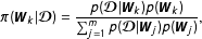 $$\begin{eqnarray}\unicode[STIX]{x1D70B}(\boldsymbol{W}_{k}|\boldsymbol{{\mathcal{D}}})=\frac{p(\boldsymbol{{\mathcal{D}}}|\boldsymbol{W}_{k})p(\boldsymbol{W}_{k})}{\mathop{\sum }_{j=1}^{m}p(\boldsymbol{{\mathcal{D}}}|\boldsymbol{W}_{j})p(\boldsymbol{W}_{j})},\end{eqnarray}$$
where $p(\boldsymbol{W}_{k})$
and
$p(\boldsymbol{W}_{k})$
and $p(\boldsymbol{W}_{j})$
represent prior model probabilities. A common choice representing little prior knowledge is to assign a prior probability of
$p(\boldsymbol{W}_{j})$
represent prior model probabilities. A common choice representing little prior knowledge is to assign a prior probability of $1/m$
to all models (Hoeting et al.
Reference Hoeting, Madigan, Raftery and Volinsky1999). Since the set of feasible networks is discrete, the denominator in Equation (4) is summed rather than integrated. Note also that this quantity is of interest for both, model selection and model averaging since it represents the relative support for one specific network as compared to the alternative network specifications in
$1/m$
to all models (Hoeting et al.
Reference Hoeting, Madigan, Raftery and Volinsky1999). Since the set of feasible networks is discrete, the denominator in Equation (4) is summed rather than integrated. Note also that this quantity is of interest for both, model selection and model averaging since it represents the relative support for one specific network as compared to the alternative network specifications in $\boldsymbol{{\mathcal{W}}}$
, given the data. For model selection, the network with the highest posterior model probability is selected. For model averaging, the posterior model probabilities serve as weights for the parameter estimates of all models. The averaged estimate of one parameter
$\boldsymbol{{\mathcal{W}}}$
, given the data. For model selection, the network with the highest posterior model probability is selected. For model averaging, the posterior model probabilities serve as weights for the parameter estimates of all models. The averaged estimate of one parameter $\unicode[STIX]{x1D703}^{l}$
is obtained by summing over all models’ parameter estimates weighted by the respective posterior model probability:
$\unicode[STIX]{x1D703}^{l}$
is obtained by summing over all models’ parameter estimates weighted by the respective posterior model probability:
 $$\begin{eqnarray}E(\unicode[STIX]{x1D703}_{avg}^{l}|\boldsymbol{{\mathcal{D}}})=\mathop{\sum }_{j=1}^{m}\unicode[STIX]{x1D70B}_{j}E(\unicode[STIX]{x1D703}^{l}|\boldsymbol{{\mathcal{D}}},\boldsymbol{W}_{j}).\end{eqnarray}$$
The variance of $\unicode[STIX]{x1D703}_{avg}^{l}$
, which is unconditional on a specific network, consists of two parts. The first part is the weighted average of the posterior variances under each model. The second part is a weighted average of the squared deviations between each model’s posterior mean and the BMA estimate (Bartels Reference Bartels1997, 644–645):
$\unicode[STIX]{x1D703}_{avg}^{l}$
, which is unconditional on a specific network, consists of two parts. The first part is the weighted average of the posterior variances under each model. The second part is a weighted average of the squared deviations between each model’s posterior mean and the BMA estimate (Bartels Reference Bartels1997, 644–645):
 $$\begin{eqnarray}\displaystyle \text{Var}(\unicode[STIX]{x1D703}_{avg}^{l}|\boldsymbol{{\mathcal{D}}})=\mathop{\sum }_{j=1}^{m}\unicode[STIX]{x1D70B}_{j}\,\text{Var}(\unicode[STIX]{x1D703}^{l}|\boldsymbol{{\mathcal{D}}},\boldsymbol{W}_{j})+\mathop{\sum }_{j=1}^{m}\unicode[STIX]{x1D70B}_{j}(E(\unicode[STIX]{x1D703}^{l}|\boldsymbol{{\mathcal{D}}},\boldsymbol{W}_{j})-E(\unicode[STIX]{x1D703}_{avg}^{l}|\boldsymbol{{\mathcal{D}}}))^{2}. & & \displaystyle\end{eqnarray}$$
Whereas in most instances it is not necessary to compute the marginal likelihood since it is possible to drop the normalizing constant and use the proportionality of $p(\unicode[STIX]{x1D73D}|\boldsymbol{{\mathcal{D}}})\propto p(\boldsymbol{{\mathcal{D}}}|\unicode[STIX]{x1D73D})p(\unicode[STIX]{x1D73D})$
, this quantity is central to BMA. One way to handle this complication is to approximate the posterior model probabilities with transdimensional Markov Chain Monte Carlo (MCMC) methods, for example, the MCMC model composition (
$p(\unicode[STIX]{x1D73D}|\boldsymbol{{\mathcal{D}}})\propto p(\boldsymbol{{\mathcal{D}}}|\unicode[STIX]{x1D73D})p(\unicode[STIX]{x1D73D})$
, this quantity is central to BMA. One way to handle this complication is to approximate the posterior model probabilities with transdimensional Markov Chain Monte Carlo (MCMC) methods, for example, the MCMC model composition ( $MC^{3}$
) technique (e.g., Hepple Reference Hepple, LeSage and Kelley Pace2004; LeSage and Parent Reference LeSage and Parent2007). These methods simultaneously explore the parameter space and the model space. However, the implementation of these methods is a nontrivial task since it requires a careful specification of priors in order to ensure that the MCMC algorithm mixes well so that it explores the entire model space. To circumvent these practical problems, I use a method developed by Chib (Reference Chib1995) for obtaining the marginal likelihood.
$MC^{3}$
) technique (e.g., Hepple Reference Hepple, LeSage and Kelley Pace2004; LeSage and Parent Reference LeSage and Parent2007). These methods simultaneously explore the parameter space and the model space. However, the implementation of these methods is a nontrivial task since it requires a careful specification of priors in order to ensure that the MCMC algorithm mixes well so that it explores the entire model space. To circumvent these practical problems, I use a method developed by Chib (Reference Chib1995) for obtaining the marginal likelihood.
Before proceeding, it is important to discuss the weaknesses of BMA. Since it requires the identification of a set of feasible models and is computationally demanding, BMA becomes increasingly impractical as the set of feasible alternatives grows. It is therefore almost impossible to test all possible combinations of covariates and all assumptions necessary to specify a model since the size of the model space quickly exceeds beyond the limits of implementability (Neumayer and Plümper Reference Neumayer and Plümper2017, 72). By the same token, BMA is difficult to implement for complex model structures (e.g., Cranmer, Rice, and Siverson Reference Cranmer, Rice and Siverson2017). It is not the most powerful tool for model selection as there are alternative algorithms that can handle complex model structures in a fast and efficient manner (e.g., Piribauer and Crespo Cuaresma Reference Piribauer and Crespo Cuaresma2016). Finally, while BMA relaxes the restrictive assumption implicitly underlying most empirical studies that one model adequately represents the true DGP, the results are conditional on the model space. Consequently, BMA requires some prior knowledge as it assumes that at least one model in the predefined set of feasible models represents the DGP reasonably well (Barker and Link Reference Barker and Link2015).
While acknowledging these limitations, I argue that the BMA approach has a special appeal for dealing with network uncertainty frequently encountered in political science applications of spatial econometric techniques. In most instances, it is not necessary to relax all assumptions required to specify a model at once. Instead, researchers can successively relax one assumption at a time and investigate the results’ sensitivity toward these slight modifications. As I argue above, network uncertainty is only one aspect of model uncertainty but it frequently triggers skepticism and causes a great deal of confusion about possible effects of network misspecification (e.g., Arbia and Fingleton Reference Arbia and Fingleton2008; LeSage and Pace Reference LeSage and Pace2014; Neumayer and Plümper Reference Neumayer and Plümper2016). In this specific scenario, BMA can quantify the effect of different and often arbitrary specification choices in $\boldsymbol{W}$
. Furthermore, it does not require the theory to exactly determine every detail of the spatial effect—an expectation that hardly will ever be met (Plümper and Neumayer Reference Plümper and Neumayer2010, 428). Instead, it suffices if the theory identifies a set of feasible alternatives. After all, the assumption that at least one network in the feasible set adequately represents the true system of dependencies is considerably less restrictive than assuming that the one
$\boldsymbol{W}$
. Furthermore, it does not require the theory to exactly determine every detail of the spatial effect—an expectation that hardly will ever be met (Plümper and Neumayer Reference Plümper and Neumayer2010, 428). Instead, it suffices if the theory identifies a set of feasible alternatives. After all, the assumption that at least one network in the feasible set adequately represents the true system of dependencies is considerably less restrictive than assuming that the one $\boldsymbol{W}$
specified in a single model is an accurate depiction of the true but unobservable network. Hence, BMA strikes a balance between assuming perfect prior knowledge about the true network structure, as conventional spatial regression models do, and assuming the complete absence of any theoretical guidance, as purely data-oriented procedures do.
$\boldsymbol{W}$
specified in a single model is an accurate depiction of the true but unobservable network. Hence, BMA strikes a balance between assuming perfect prior knowledge about the true network structure, as conventional spatial regression models do, and assuming the complete absence of any theoretical guidance, as purely data-oriented procedures do.
4 Alternative Approaches to Network Uncertainty
The necessity to specify $\boldsymbol{W}$
prior to model estimation is an outstanding methodological problem that attracts considerable scholarly attention by spatial econometricians (e.g., Hays, Kachi, and Franzese Reference Hays, Kachi and Franzese2010; Kostov Reference Kostov2010; Mueller and Loomis Reference Mueller and Loomis2010; Darmofal Reference Darmofal2015). Perhaps unsurprisingly, the literature offers a variety of different approaches to mitigate the apparent arbitrariness in the specification of
$\boldsymbol{W}$
prior to model estimation is an outstanding methodological problem that attracts considerable scholarly attention by spatial econometricians (e.g., Hays, Kachi, and Franzese Reference Hays, Kachi and Franzese2010; Kostov Reference Kostov2010; Mueller and Loomis Reference Mueller and Loomis2010; Darmofal Reference Darmofal2015). Perhaps unsurprisingly, the literature offers a variety of different approaches to mitigate the apparent arbitrariness in the specification of $\boldsymbol{W}$
.
$\boldsymbol{W}$
.
Zhukov and Stewart (Reference Zhukov and Stewart2013), for example, develop a three-step procedure to select a single best performing network structure among a predefined candidate pool. Their approach essentially relies on a combination of parameter-level and model-level diagnostics, where the researcher selects the $\boldsymbol{W}$
that exhibits a significant autocorrelation parameter and provides the best fit to the data based on statistics like the
$\boldsymbol{W}$
that exhibits a significant autocorrelation parameter and provides the best fit to the data based on statistics like the $R^{2}$
or the Akaike Information Criterion (AIC). In a similar vein, Kostov (Reference Kostov2010, Reference Kostov2013) proposes component-wise model-boosting to find the appropriate network structure among a predefined set of candidate networks. This algorithm has the appeal that it is comparatively fast and efficient which makes it a powerful tool for model selection (Cranmer, Rice, and Siverson Reference Cranmer, Rice and Siverson2017).
$R^{2}$
or the Akaike Information Criterion (AIC). In a similar vein, Kostov (Reference Kostov2010, Reference Kostov2013) proposes component-wise model-boosting to find the appropriate network structure among a predefined set of candidate networks. This algorithm has the appeal that it is comparatively fast and efficient which makes it a powerful tool for model selection (Cranmer, Rice, and Siverson Reference Cranmer, Rice and Siverson2017).
Yet, these techniques have some important limitations. Above all, they are exclusively suited for model selection. Model selection refers to the problem of choosing a model out of a set of candidate models. Once a model is selected, inferences are based on this model as if it has generated the data. In contrast, model averaging is the process by which a researcher combines the estimates from different models in a specific way to obtain inferences from multiple models. Thereby, model averaging adequately reflects model uncertainty in the estimates (Bartels Reference Bartels1997; Wasserman Reference Wasserman2000). Thus, if the task is to evaluate and quantify the amount of uncertainty associated with different and equally plausible specifications of $\boldsymbol{W}$
, these procedures are of limited utility. Furthermore, Kostov (Reference Kostov2010, 541) also notes that there is no guarantee that these techniques will unambiguously identify one single best performing network structure. Goodness-of-fit measures may not be able to clearly identify a best fitting model.Footnote
5
After all, if the theory regards multiple network structures as equally likely, considering only a single
$\boldsymbol{W}$
, these procedures are of limited utility. Furthermore, Kostov (Reference Kostov2010, 541) also notes that there is no guarantee that these techniques will unambiguously identify one single best performing network structure. Goodness-of-fit measures may not be able to clearly identify a best fitting model.Footnote
5
After all, if the theory regards multiple network structures as equally likely, considering only a single $\boldsymbol{W}$
is hardly justifiable, irrespective of how good it fits the sampled data.
$\boldsymbol{W}$
is hardly justifiable, irrespective of how good it fits the sampled data.
Alternatively, Neumayer and Plümper (Reference Neumayer and Plümper2016, 186) propose a semiparametric approach. Since theories of spatial dependence rarely provide sufficient information on how the spatial effect varies between different levels of connectivity, they suggest that researchers divide the connectivity variable into several discrete categories and estimate a spatial parameter for each category. Thereby, the spatial effect can vary with connectivity. Researchers do not impose a functional form on the units’ connectivity but rather estimate it from the data. At the same time, the semiparametric approach does not rule out arbitrariness in model specification as the researcher decides on the number of categories and the location of the thresholds which renders robustness tests indispensable. Practical estimation problems can also arise due to correlation between the spatial variables which will result in a loss of efficiency (Neumayer and Plümper Reference Neumayer and Plümper2016, 186).
Regarding network uncertainty, the strategy most similar to the BMA approach is the multiparametric spatiotemporal autoregressive (m-STAR) model developed by Hays, Kachi, and Franzese (Reference Hays, Kachi and Franzese2010) which includes all theoretically reasonable spatial lags in a single regression equation. While the BMA estimate of $\unicode[STIX]{x1D70C}$
is the weighted average of this parameter’s posterior distributions under each candidate network, the m-STAR model estimates a separate parameter for each network configuration. Thereby, it directly accounts for the possibly multidimensional nature of connectivity.Footnote
6
However, if the alternative network structures are similar—i.e., because connectivity is unidimensional—the spatial lags might be highly collinear, which inflates the standard errors or entirely impedes the estimation of the spatial parameters in the m-STAR model. In contrast, since the BMA approach features a single spatial lag in each regression equation, multicollinearity does not cause estimation problems.
$\unicode[STIX]{x1D70C}$
is the weighted average of this parameter’s posterior distributions under each candidate network, the m-STAR model estimates a separate parameter for each network configuration. Thereby, it directly accounts for the possibly multidimensional nature of connectivity.Footnote
6
However, if the alternative network structures are similar—i.e., because connectivity is unidimensional—the spatial lags might be highly collinear, which inflates the standard errors or entirely impedes the estimation of the spatial parameters in the m-STAR model. In contrast, since the BMA approach features a single spatial lag in each regression equation, multicollinearity does not cause estimation problems.
While all of the procedures discussed so far—including BMA—rely on some theoretical considerations, e.g., to identify a set of feasible networks, other approaches attempt to address network uncertainty from a purely data-oriented perspective. Bhattacharjee and Jensen-Butler (Reference Bhattacharjee and Jensen-Butler2013), for example, develop an estimator that uses the observed spatial autocovariance to estimate the elements of $\boldsymbol{W}$
. In a similar vein, Ahrens and Bhattacharjee (Reference Ahrens and Bhattacharjee2015) propose a two-step least absolute shrinkage and selection operator (LASSO) to estimate the unknown network structure. Although procedures to estimate
$\boldsymbol{W}$
. In a similar vein, Ahrens and Bhattacharjee (Reference Ahrens and Bhattacharjee2015) propose a two-step least absolute shrinkage and selection operator (LASSO) to estimate the unknown network structure. Although procedures to estimate $\boldsymbol{W}$
from the data do not require prior knowledge of the network of dependencies, their practical utility for social science research is restricted by some notable limitations. Political scientists employing spatial econometric techniques to test theoretical expectations are interested in assessing the empirical support for theories of interdependence instead of merely fitting a model as closely as possible to sampled data. Insofar as researchers wish to draw conclusions with respect to these theories, estimating
$\boldsymbol{W}$
from the data do not require prior knowledge of the network of dependencies, their practical utility for social science research is restricted by some notable limitations. Political scientists employing spatial econometric techniques to test theoretical expectations are interested in assessing the empirical support for theories of interdependence instead of merely fitting a model as closely as possible to sampled data. Insofar as researchers wish to draw conclusions with respect to these theories, estimating $\boldsymbol{W}$
does not constitute a valuable solution to the problem of network uncertainty as it only provides information about empirical patterns of spatial autocorrelation. Neither does it permit meaningful inferences concerning the validity of theories of interdependence nor can researchers differentiate between potential causes of spatial dependence without further analyses (Bhattacharjee and Jensen-Butler Reference Bhattacharjee and Jensen-Butler2013, 624).
$\boldsymbol{W}$
does not constitute a valuable solution to the problem of network uncertainty as it only provides information about empirical patterns of spatial autocorrelation. Neither does it permit meaningful inferences concerning the validity of theories of interdependence nor can researchers differentiate between potential causes of spatial dependence without further analyses (Bhattacharjee and Jensen-Butler Reference Bhattacharjee and Jensen-Butler2013, 624).
5 Monte Carlo Experiments
To investigate the effects of different forms of misspecification in $\boldsymbol{W}$
relevant for applied research and to assess the performance of BMA, this section presents two Monte Carlo studies. The true DGP in the simulations is the standard SAR model in its reduced form:
$\boldsymbol{W}$
relevant for applied research and to assess the performance of BMA, this section presents two Monte Carlo studies. The true DGP in the simulations is the standard SAR model in its reduced form:
 $$\begin{eqnarray}\boldsymbol{y}=(\boldsymbol{I}_{n}-\unicode[STIX]{x1D70C}\boldsymbol{W})^{-1}(\unicode[STIX]{x1D6FC}\unicode[STIX]{x1D73E}_{n}+\boldsymbol{x}\unicode[STIX]{x1D6FD})+(\boldsymbol{I}_{n}-\unicode[STIX]{x1D70C}\boldsymbol{W})^{-1}\unicode[STIX]{x1D750}.\end{eqnarray}$$
By way of illustration, I only include a single regressor. Using Equation (7), I generate 1,000 simulations of $\boldsymbol{y}$
with a sample size of
$\boldsymbol{y}$
with a sample size of $n=100$
. Like the residual vector
$n=100$
. Like the residual vector $\unicode[STIX]{x1D750}$
, the covariate vector
$\unicode[STIX]{x1D750}$
, the covariate vector $\boldsymbol{x}$
contains
$\boldsymbol{x}$
contains $n$
i.i.d. draws from a standard normal distribution. The coefficients
$n$
i.i.d. draws from a standard normal distribution. The coefficients $\unicode[STIX]{x1D6FC}=3$
and
$\unicode[STIX]{x1D6FC}=3$
and $\unicode[STIX]{x1D6FD}=2$
are held constant across all Monte Carlos while I separately simulate a scenario featuring low and high levels of cross-sectional dependence:
$\unicode[STIX]{x1D6FD}=2$
are held constant across all Monte Carlos while I separately simulate a scenario featuring low and high levels of cross-sectional dependence: $\unicode[STIX]{x1D70C}=\{0.2;0.8\}$
. Due to the endogeneity present in the model, the interpretation of substantive effects becomes more complex compared to standard linear regression models. The partial derivative of
$\unicode[STIX]{x1D70C}=\{0.2;0.8\}$
. Due to the endogeneity present in the model, the interpretation of substantive effects becomes more complex compared to standard linear regression models. The partial derivative of $\boldsymbol{y}$
with respect to
$\boldsymbol{y}$
with respect to $\boldsymbol{x}$
is not simply
$\boldsymbol{x}$
is not simply $\unicode[STIX]{x1D6FD}$
but
$\unicode[STIX]{x1D6FD}$
but $\unicode[STIX]{x2202}\boldsymbol{y}/\unicode[STIX]{x2202}\boldsymbol{x}=(\boldsymbol{I}_{n}-\unicode[STIX]{x1D70C}\boldsymbol{W})^{-1}\unicode[STIX]{x1D6FD}$
. This partial derivatives matrix contains the direct impact of a one-unit change in
$\unicode[STIX]{x2202}\boldsymbol{y}/\unicode[STIX]{x2202}\boldsymbol{x}=(\boldsymbol{I}_{n}-\unicode[STIX]{x1D70C}\boldsymbol{W})^{-1}\unicode[STIX]{x1D6FD}$
. This partial derivatives matrix contains the direct impact of a one-unit change in $x_{i}$
on
$x_{i}$
on $y_{i}$
on its diagonal as well as its indirect impact on all other units
$y_{i}$
on its diagonal as well as its indirect impact on all other units $y_{j\neq i}$
on its off-diagonal. The sum of these quantities yields the total impact for unit
$y_{j\neq i}$
on its off-diagonal. The sum of these quantities yields the total impact for unit $i$
. As LeSage and Pace (Reference LeSage and Pace2009, 39) suggest, I report average impacts as summary statistics in the Monte Carlo studies:Footnote
7
$i$
. As LeSage and Pace (Reference LeSage and Pace2009, 39) suggest, I report average impacts as summary statistics in the Monte Carlo studies:Footnote
7
 $$\begin{eqnarray}\begin{array}{@{}rcl@{}}\text{Direct}\ & =\ & n^{-1}\text{tr}((\boldsymbol{I}_{n}-\unicode[STIX]{x1D70C}\boldsymbol{W})^{-1}\unicode[STIX]{x1D6FD}),\\ \text{Indirect}\ & =\ & n^{-1}[\unicode[STIX]{x1D73E}_{n}^{\prime }((\boldsymbol{I}_{n}-\unicode[STIX]{x1D70C}\boldsymbol{W})^{-1}\unicode[STIX]{x1D6FD})\unicode[STIX]{x1D73E}_{n}-\text{tr}((\boldsymbol{I}_{n}-\unicode[STIX]{x1D70C}\boldsymbol{W})^{-1}\unicode[STIX]{x1D6FD})].\end{array}\end{eqnarray}$$
I conduct two experiments which are designed to resemble different forms of network uncertainty commonly encountered in empirical studies, including both replication studies presented below: (i) uncertainty about the neighborhood definition and (ii) uncertainty about the functional form or the weighting scheme (e.g., Kostov Reference Kostov2010; Williams Reference Williams2015).Footnote 8
5.1 Study 1: misspecification in the neighborhood definition
In many applications of spatial econometric techniques, researchers are uncertain about which units are connected to each other (e.g., Beck, Gleditsch, and Beardsley Reference Beck, Gleditsch and Beardsley2006; Gleditsch and Ward Reference Gleditsch and Ward2006; Darmofal Reference Darmofal2015). Thus, understanding the consequences of misspecifying the units’ neighborhood is of great practical importance. Assuming that the units are ordered on one dimension, I specify the true binary connectivity matrix such that its elements $w_{i,j}$
take on a value of 1 if unit
$w_{i,j}$
take on a value of 1 if unit $j$
belongs to
$j$
belongs to $i$
’s five nearest neighbors on each side and zero otherwise.Footnote
9
To make the estimates comparable across the network specifications and to ensure the invertibility of
$i$
’s five nearest neighbors on each side and zero otherwise.Footnote
9
To make the estimates comparable across the network specifications and to ensure the invertibility of $\boldsymbol{W}$
, I employ a min–max normalization and divide each cell in
$\boldsymbol{W}$
, I employ a min–max normalization and divide each cell in $\boldsymbol{W}$
by the constant
$\boldsymbol{W}$
by the constant $\unicode[STIX]{x1D70F}=\min \{\max (r),\max (c)\}$
, where
$\unicode[STIX]{x1D70F}=\min \{\max (r),\max (c)\}$
, where $\max (r)$
is the largest row sum and
$\max (r)$
is the largest row sum and $\max (c)$
is the largest column sum (Kelejian and Prucha Reference Kelejian and Prucha2010, 56).Footnote
10
$\max (c)$
is the largest column sum (Kelejian and Prucha Reference Kelejian and Prucha2010, 56).Footnote
10
In order to investigate the bias induced by uncertainty about the number of neighbors, I construct ten different connectivity matrices, $\boldsymbol{W}_{1}$
to
$\boldsymbol{W}_{1}$
to $\boldsymbol{W}_{10}$
, where
$\boldsymbol{W}_{10}$
, where $\boldsymbol{W}_{1}$
connects each unit to its adjacent neighbor on both sides,
$\boldsymbol{W}_{1}$
connects each unit to its adjacent neighbor on both sides, $\boldsymbol{W}_{2}$
connects each unit to the two closest neighbors on each side, and so on. Before estimating the SAR model in Equation (1) using the different matrices and the artificially generated data, I apply the min–max normalization.Footnote
11
$\boldsymbol{W}_{2}$
connects each unit to the two closest neighbors on each side, and so on. Before estimating the SAR model in Equation (1) using the different matrices and the artificially generated data, I apply the min–max normalization.Footnote
11
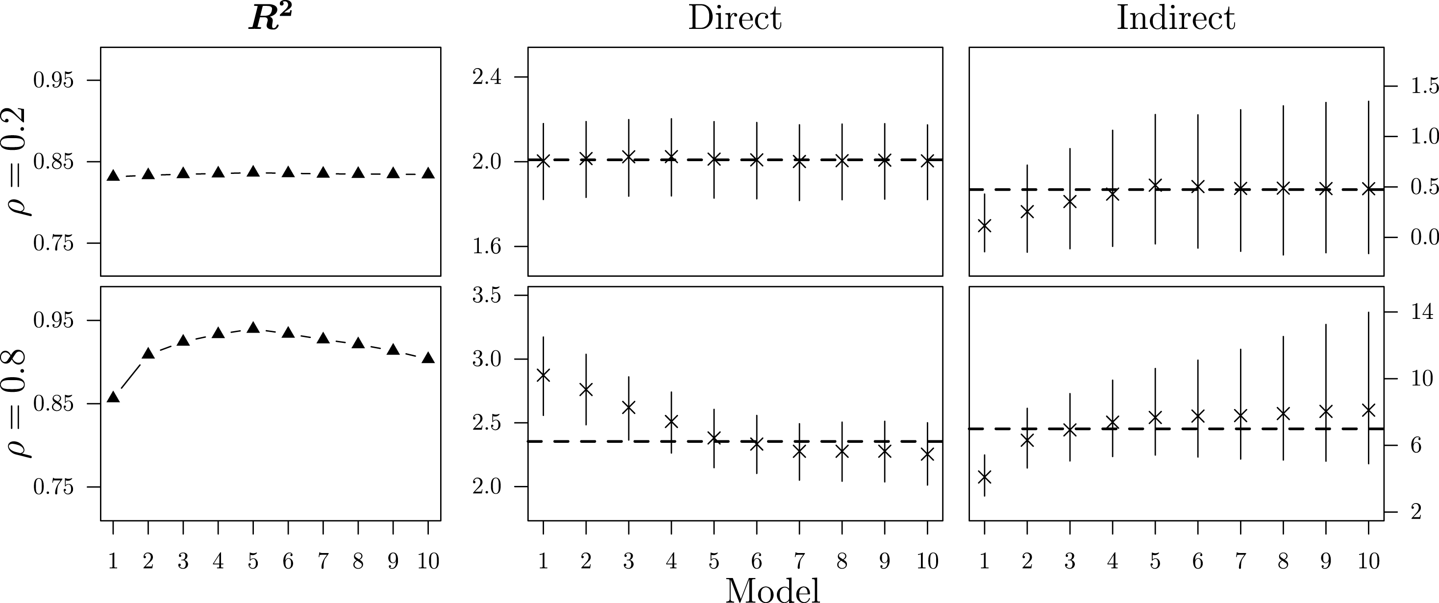
Figure 1. $R^{2}$
, average direct, and average indirect impacts across 1,000 simulations.
$R^{2}$
, average direct, and average indirect impacts across 1,000 simulations.
By taking the popular $R^{2}$
as an example, Figure 1 exemplifies the inability of classical goodness-of-fit measures to identify
$R^{2}$
as an example, Figure 1 exemplifies the inability of classical goodness-of-fit measures to identify $\boldsymbol{W}_{5}$
as the true network structure. Even in the high-dependency scenario, there are only minor differences between the specifications which complicates the selection of the correct
$\boldsymbol{W}_{5}$
as the true network structure. Even in the high-dependency scenario, there are only minor differences between the specifications which complicates the selection of the correct $\boldsymbol{W}$
and inhibits the successful application of the three-step procedure discussed in Section 4. Additionally, Figure 1 reports the means of the average direct and indirect impacts across the 1,000 simulations together with the respective 95% highest density area and compares them to the true effects, represented by the dashed horizontal lines.Footnote
12
In the low-dependency scenario, there are only minor differences between the alternative
$\boldsymbol{W}$
and inhibits the successful application of the three-step procedure discussed in Section 4. Additionally, Figure 1 reports the means of the average direct and indirect impacts across the 1,000 simulations together with the respective 95% highest density area and compares them to the true effects, represented by the dashed horizontal lines.Footnote
12
In the low-dependency scenario, there are only minor differences between the alternative $\boldsymbol{W}$
s. While the estimated direct impact remains almost identical, considering too few neighbors downwardly biases the estimate of the average indirect impact. At the same time, applying a broad neighborhood definition that includes more units than the true underlying network does not bias the substantive effect estimates. In the high-dependency scenario, the differences between the ten network specifications become more pronounced. If the neighborhood definition is too narrow, the estimated direct impact will be upwardly biased and the indirect impact downwardly biased. Again, considering too many units as being part of a unit’s neighborhood does not bias the estimates. Yet, it increases the variation in the estimates of the average indirect impact across the simulation trials, making inferences more vulnerable to random fluctuations.
$\boldsymbol{W}$
s. While the estimated direct impact remains almost identical, considering too few neighbors downwardly biases the estimate of the average indirect impact. At the same time, applying a broad neighborhood definition that includes more units than the true underlying network does not bias the substantive effect estimates. In the high-dependency scenario, the differences between the ten network specifications become more pronounced. If the neighborhood definition is too narrow, the estimated direct impact will be upwardly biased and the indirect impact downwardly biased. Again, considering too many units as being part of a unit’s neighborhood does not bias the estimates. Yet, it increases the variation in the estimates of the average indirect impact across the simulation trials, making inferences more vulnerable to random fluctuations.
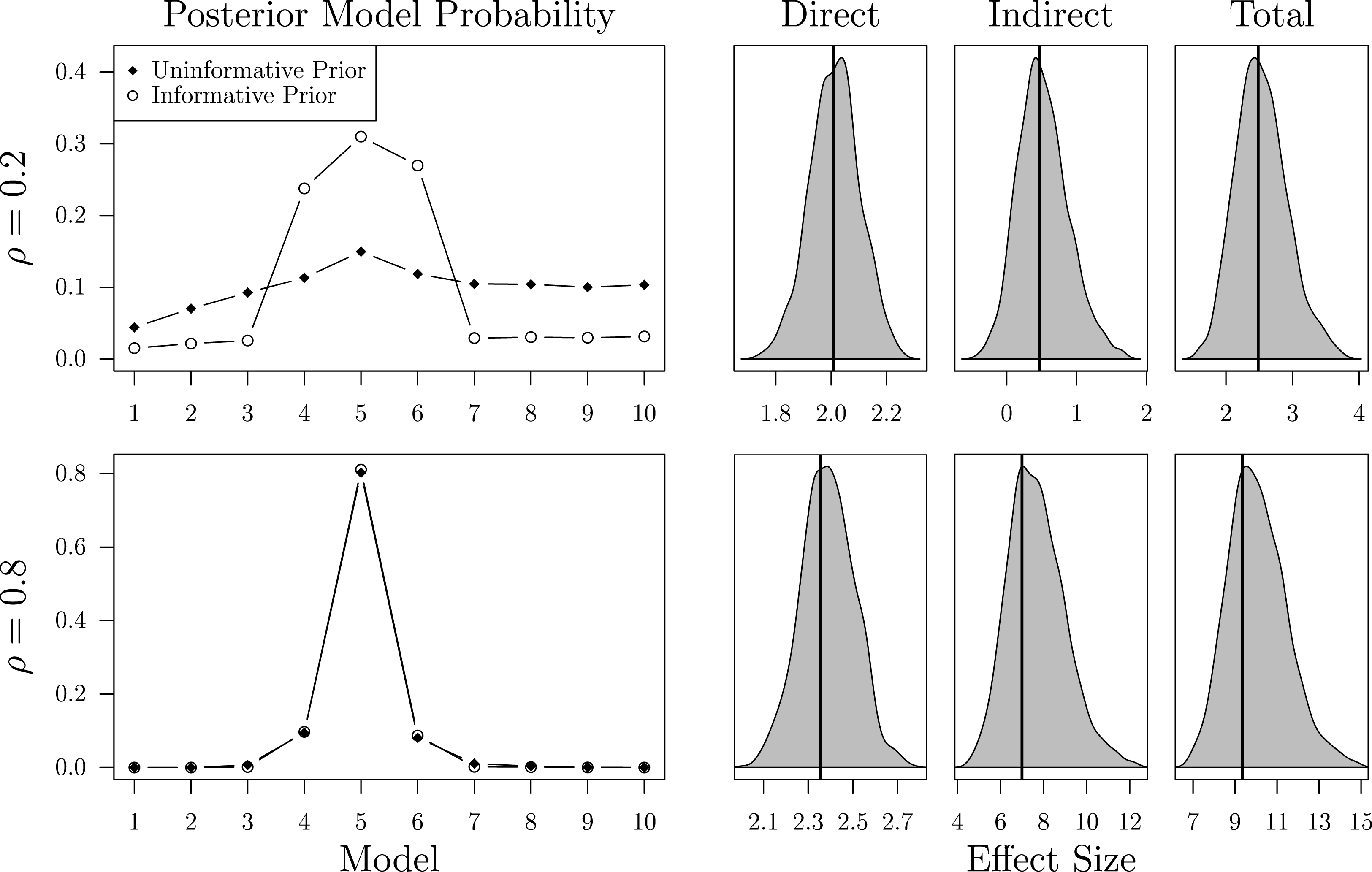
Figure 2. BMA estimates: posterior model probabilities, average direct, indirect, and total impacts.
To evaluate the performance of BMA, suppose that a researcher interested in the effect of $\boldsymbol{x}$
on the artificial outcome vector
$\boldsymbol{x}$
on the artificial outcome vector $\boldsymbol{y}$
is uncertain about the correct number of neighbors. Since her theory considers each of the ten network specifications as equally likely, she assigns an uninformative prior probability of 0.1 to each of them. The upper part of Figure 2 presents the average posterior model probabilities together with the density of the effect estimates across all simulations for the low-dependency scenario. Although BMA correctly identifies
$\boldsymbol{y}$
is uncertain about the correct number of neighbors. Since her theory considers each of the ten network specifications as equally likely, she assigns an uninformative prior probability of 0.1 to each of them. The upper part of Figure 2 presents the average posterior model probabilities together with the density of the effect estimates across all simulations for the low-dependency scenario. Although BMA correctly identifies $\boldsymbol{W}_{5}$
as the most likely network, it is on average only 3.11% more likely than
$\boldsymbol{W}_{5}$
as the most likely network, it is on average only 3.11% more likely than $\boldsymbol{W}_{6}$
. Yet, given that the effect estimates of all models in the set of feasible alternatives do not notably differ, BMA provides accurate estimates of the substantive effects. In the case of strong cross-sectional dependence, as depicted in the lower part of Figure 2, BMA unambiguously identifies
$\boldsymbol{W}_{6}$
. Yet, given that the effect estimates of all models in the set of feasible alternatives do not notably differ, BMA provides accurate estimates of the substantive effects. In the case of strong cross-sectional dependence, as depicted in the lower part of Figure 2, BMA unambiguously identifies $\boldsymbol{W}_{5}$
as the true network. Still, the effect estimates are slightly inflated as a result of the simultaneity bias which is especially severe if the interdependence is strong (Franzese and Hays Reference Franzese and Hays2007).
$\boldsymbol{W}_{5}$
as the true network. Still, the effect estimates are slightly inflated as a result of the simultaneity bias which is especially severe if the interdependence is strong (Franzese and Hays Reference Franzese and Hays2007).
The left part of Figure 2 also demonstrates the effect of incorporating prior knowledge about the likelihood of each $\boldsymbol{W}$
. Instead of considering each of the candidate networks as equally likely, suppose the researcher’s prior belief that the true network is either
$\boldsymbol{W}$
. Instead of considering each of the candidate networks as equally likely, suppose the researcher’s prior belief that the true network is either $\boldsymbol{W}_{4}$
,
$\boldsymbol{W}_{4}$
, $\boldsymbol{W}_{5}$
, or
$\boldsymbol{W}_{5}$
, or $\boldsymbol{W}_{6}$
is 0.8. While this more informative prior changes the average posterior model probability of the true network
$\boldsymbol{W}_{6}$
is 0.8. While this more informative prior changes the average posterior model probability of the true network $\boldsymbol{W}_{5}$
from 14.96% to 31% in the low-dependency scenario, it hardly affects the posterior probability in the high-dependency scenario. The effect of prior model probabilities decreases as
$\boldsymbol{W}_{5}$
from 14.96% to 31% in the low-dependency scenario, it hardly affects the posterior probability in the high-dependency scenario. The effect of prior model probabilities decreases as $\unicode[STIX]{x1D70C}$
increases.
$\unicode[STIX]{x1D70C}$
increases.
In sum, the importance of correctly specifying $\boldsymbol{W}$
increases with the strength of the cross-sectional dependence in the data. This Monte Carlo experiment shows that defining the neighborhood too narrowly attenuates the estimates of the average indirect impact. A broad neighborhood definition does not bias the estimates but increases their variability. Overall, however, the effect of a misspecification in the neighborhood definition on the estimated substantive effects is rather small and BMA provides correct effect estimates.
$\boldsymbol{W}$
increases with the strength of the cross-sectional dependence in the data. This Monte Carlo experiment shows that defining the neighborhood too narrowly attenuates the estimates of the average indirect impact. A broad neighborhood definition does not bias the estimates but increases their variability. Overall, however, the effect of a misspecification in the neighborhood definition on the estimated substantive effects is rather small and BMA provides correct effect estimates.
5.2 Study 2: misspecification in the weighting scheme
Another source of network uncertainty frequently encountered in empirical applications concerns the strength of the cross-sectional dependence (e.g., Plümper and Neumayer Reference Plümper and Neumayer2010; Williams Reference Williams2015; Juhl Reference Juhl2018). The necessity to specify $\boldsymbol{W}$
prior to estimation requires researchers to conceptualize the strength of the relationships among the units and to define their functional form or their weighting scheme (Kostov Reference Kostov2010, 535). This Monte Carlo study investigates the effect of network uncertainty stemming from uncertainty in the functional form of
$\boldsymbol{W}$
prior to estimation requires researchers to conceptualize the strength of the relationships among the units and to define their functional form or their weighting scheme (Kostov Reference Kostov2010, 535). This Monte Carlo study investigates the effect of network uncertainty stemming from uncertainty in the functional form of $\boldsymbol{W}$
.
$\boldsymbol{W}$
.
Suppose that the $n=100$
units are ordered on a single dimension with an equal distance of
$n=100$
units are ordered on a single dimension with an equal distance of $d=10$
on an arbitrary scale between adjacent units. Furthermore, assume that the true network structure in the DGP connects all units within a radius of
$d=10$
on an arbitrary scale between adjacent units. Furthermore, assume that the true network structure in the DGP connects all units within a radius of $d=50$
and that the true weighting scheme is the inverse distance between two connected units:
$d=50$
and that the true weighting scheme is the inverse distance between two connected units: $w_{i,j}=1/d_{i,j}~\forall ~d_{i,j}\leqslant 50$
. However, while the theory correctly predicts interdependencies within a radius of
$w_{i,j}=1/d_{i,j}~\forall ~d_{i,j}\leqslant 50$
. However, while the theory correctly predicts interdependencies within a radius of $d=50$
, it does not specify the exact functional form of
$d=50$
, it does not specify the exact functional form of $\boldsymbol{W}$
. Therefore, I define six different weighting schemes, including all schemes applied by Plümper and Neumayer (Reference Plümper and Neumayer2010). In line with the theory, the matrices connect all units within a radius of
$\boldsymbol{W}$
. Therefore, I define six different weighting schemes, including all schemes applied by Plümper and Neumayer (Reference Plümper and Neumayer2010). In line with the theory, the matrices connect all units within a radius of $d=50$
and only differ in the specification of the connections’ relative strengths.Footnote
13
Besides the true inverse distance specification, the set of alternative networks consists of a binary connectivity matrix, a contiguity matrix, an inverse logarithmic distance specification, an inverse reversed distance specification, and an inverse squared distance specification. Again, to ease interpretation and to assure the invertibility of
$d=50$
and only differ in the specification of the connections’ relative strengths.Footnote
13
Besides the true inverse distance specification, the set of alternative networks consists of a binary connectivity matrix, a contiguity matrix, an inverse logarithmic distance specification, an inverse reversed distance specification, and an inverse squared distance specification. Again, to ease interpretation and to assure the invertibility of $\boldsymbol{W}$
, all matrices are min–max normalized.
$\boldsymbol{W}$
, all matrices are min–max normalized.

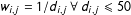
Figure 3. Spatial parameter estimates and average total impacts across 1,000 simulations.
The left part of Figure 3 shows the estimate of the spatial parameter across all alternative specifications. Clearly, the varying $\hat{\unicode[STIX]{x1D70C}}$
in both the low-dependency but especially in the high-dependency scenario suggests that model misspecification can severely distort inferences. Yet, as LeSage and Pace (Reference LeSage and Pace2014) emphasize, differences in
$\hat{\unicode[STIX]{x1D70C}}$
in both the low-dependency but especially in the high-dependency scenario suggests that model misspecification can severely distort inferences. Yet, as LeSage and Pace (Reference LeSage and Pace2014) emphasize, differences in $\hat{\unicode[STIX]{x1D70C}}$
do not necessarily imply differences in the substantive effects. In fact, the right part of Figure 3 illustrates that, despite differences in
$\hat{\unicode[STIX]{x1D70C}}$
do not necessarily imply differences in the substantive effects. In fact, the right part of Figure 3 illustrates that, despite differences in $\hat{\unicode[STIX]{x1D70C}}$
, the estimated average total impact of the regressor is almost identical across the specifications in both scenarios. Except for the simple contiguity matrix which also implies a different neighborhood definition, these results suggest that this type of network uncertainty does not bias the substantive effect estimates.Footnote
14
$\hat{\unicode[STIX]{x1D70C}}$
, the estimated average total impact of the regressor is almost identical across the specifications in both scenarios. Except for the simple contiguity matrix which also implies a different neighborhood definition, these results suggest that this type of network uncertainty does not bias the substantive effect estimates.Footnote
14

Figure 4. BMA estimates: posterior model probabilities and average total impacts.
Unsurprisingly, Figure 4 shows that BMA also performs well in this second Monte Carlo study. Irrespective of the strength of the cross-sectional dependence, the correctly specified $\boldsymbol{W}$
has the highest posterior model probability—although three specifications are almost equally likely in the low-dependency scenario, given that all specifications have the same prior probability. More importantly, despite uncertainty about the functional form of the dependence, BMA provides accurate effect estimates in this simulation study as well. Similar to the results presented in the first Monte Carlo experiment, BMA reliably recovers the true effect size.
$\boldsymbol{W}$
has the highest posterior model probability—although three specifications are almost equally likely in the low-dependency scenario, given that all specifications have the same prior probability. More importantly, despite uncertainty about the functional form of the dependence, BMA provides accurate effect estimates in this simulation study as well. Similar to the results presented in the first Monte Carlo experiment, BMA reliably recovers the true effect size.
Taken together, and in line with the analytical results presented by LeSage and Pace (Reference LeSage and Pace2014), both Monte Carlo experiments performed here indicate that network uncertainty is a less severe concern than commonly expected in applied settings. While the parameter estimates depend on $\boldsymbol{W}$
, the substantive effect estimates are little affected by a misspecification in the network structure. Moreover, these simulations also provide evidence for the ability of BMA to accommodate network uncertainty and to derive unbiased effect estimates even in a situation where single network specifications yield biased estimates.
$\boldsymbol{W}$
, the substantive effect estimates are little affected by a misspecification in the network structure. Moreover, these simulations also provide evidence for the ability of BMA to accommodate network uncertainty and to derive unbiased effect estimates even in a situation where single network specifications yield biased estimates.
6 Political Science Applications
In order to demonstrate the utility of the BMA approach in political science applications using spatial econometric techniques, this section presents two replication studies from different subfields of the discipline. It also considers the alternative approaches advocated by Zhukov and Stewart (Reference Zhukov and Stewart2013) and Neumayer and Plümper (Reference Neumayer and Plümper2016) discussed in Section 4 and illustrates how BMA compensates the weaknesses of these approaches.Footnote 15
The first example replicates a study by Gleditsch and Ward (Reference Gleditsch and Ward2006) on the international diffusion of democratization and shows how BMA performs under different neighboring criteria commonly employed in the subfield of International Relations. The second example is a reexamination of a study conducted by Plümper and Neumayer (Reference Plümper and Neumayer2010), who show how spatial parameter estimates are sensitive to different specifications of the weighting scheme. Besides their publication in influential journals and the availability of excellently documented replication materials, different substantive and illustrative considerations motivate the selection of these specific studies.
First, the studies are located in different subfields of the discipline—International Relations and International Political Economy—and feature different forms of network uncertainty that can be considered archetypical. Second, the authors are explicit about the problems they face when specifying $\boldsymbol{W}$
and discuss their choices. Finally, each of the articles identifies a set of feasible network specifications based on theoretical considerations. This is important since, as discussed in Section 3, the composition of the set of alternative models is a crucial step in the BMA approach (see also Barker and Link Reference Barker and Link2015; Cranmer, Rice, and Siverson Reference Cranmer, Rice and Siverson2017).
$\boldsymbol{W}$
and discuss their choices. Finally, each of the articles identifies a set of feasible network specifications based on theoretical considerations. This is important since, as discussed in Section 3, the composition of the set of alternative models is a crucial step in the BMA approach (see also Barker and Link Reference Barker and Link2015; Cranmer, Rice, and Siverson Reference Cranmer, Rice and Siverson2017).
6.1 Application I: the diffusion of democratization
By replicating the influential study by Gleditsch and Ward (Reference Gleditsch and Ward2006), I demonstrate the effect of uncertainty about the neighborhood definition—a situation regularly encountered by scholars working in the field of International Relations.
Starting with the observation that democratic regimes and transitions to democracy cluster geographically, the authors are interested in transnational spillover effects of regime types. Their theoretical expectation is that autocratic regimes are more likely to become democratic if the share of democratic countries in their neighborhood increases and if at least one neighboring country undergoes a transition to democracy. In order to test these propositions, Gleditsch and Ward (Reference Gleditsch and Ward2006) analyze changes in regime type as a first-order Markov process with a binary outcome and estimate a transition model that contains spatial lags with the following transition matrix:
 $$\begin{eqnarray}\boldsymbol{T}=\left(\begin{array}{@{}ll@{}}\Pr (D\rightarrow D)\quad & \Pr (D\rightarrow A)\\ \Pr (A\rightarrow D)\quad & \Pr (A\rightarrow A)\end{array}\right).\end{eqnarray}$$
The authors use a probit model to estimate the transition probabilities from time $t-1$
to
$t-1$
to $t$
for each observation
$t$
for each observation $i$
conditional on the covariate vector
$i$
conditional on the covariate vector $\boldsymbol{x}_{i,t}$
:
$\boldsymbol{x}_{i,t}$
:
 $$\begin{eqnarray}\Pr (y_{i,t}=1|y_{i,t-1},\boldsymbol{x}_{i,t},\boldsymbol{W}_{i,t})=\unicode[STIX]{x1D6F7}(\boldsymbol{x}_{i,t}^{\prime }\unicode[STIX]{x1D737}+\unicode[STIX]{x1D70C}_{1}\boldsymbol{W}_{i,t}\boldsymbol{y}_{t-1}+y_{i,t-1}\boldsymbol{x}_{i,t}^{\prime }\unicode[STIX]{x1D736}+y_{i,t-1}\unicode[STIX]{x1D70C}_{2}\boldsymbol{W}_{i,t}\boldsymbol{y}_{t-1}),\end{eqnarray}$$
where $y_{i,t}=1$
if country
$y_{i,t}=1$
if country $i$
is autocratic at time
$i$
is autocratic at time $t$
. The covariate vector also contains an indicator variable signifying whether a transition to democracy takes place in at least one country in the neighborhood network
$t$
. The covariate vector also contains an indicator variable signifying whether a transition to democracy takes place in at least one country in the neighborhood network $\boldsymbol{W}_{i,t}$
. Since
$\boldsymbol{W}_{i,t}$
. Since $\boldsymbol{W}$
is row-standardized, the spatial lag represents the proportion of democratic countries in the neighborhood. In their model, each parameter in the coefficient vector
$\boldsymbol{W}$
is row-standardized, the spatial lag represents the proportion of democratic countries in the neighborhood. In their model, each parameter in the coefficient vector $\unicode[STIX]{x1D737}$
indicates the effect of the respective covariate on a democracy’s transition probability to autocracy:
$\unicode[STIX]{x1D737}$
indicates the effect of the respective covariate on a democracy’s transition probability to autocracy: $\Pr (D\rightarrow A)$
. The covariates’ effect on the probability of remaining an autocratic regime is given by
$\Pr (D\rightarrow A)$
. The covariates’ effect on the probability of remaining an autocratic regime is given by $\unicode[STIX]{x1D738}=\unicode[STIX]{x1D736}+\unicode[STIX]{x1D737}$
. Since the probabilities for all possible outcomes at time
$\unicode[STIX]{x1D738}=\unicode[STIX]{x1D736}+\unicode[STIX]{x1D737}$
. Since the probabilities for all possible outcomes at time $t$
must sum to unity, the probability of a transition from autocracy to democracy can be calculated by
$t$
must sum to unity, the probability of a transition from autocracy to democracy can be calculated by $1-\Pr (A\rightarrow A)$
.
$1-\Pr (A\rightarrow A)$
.
Yet, the definition of a country’s “regional context” or “neighborhood” is ambiguous which complicates the specification of $\boldsymbol{W}$
and gives rise to concerns about network uncertainty. While noting the arbitrariness of their choice, Gleditsch and Ward (Reference Gleditsch and Ward2006, 922–923) define the states’ neighborhood by the countries within a radius of 500 km.Footnote
16
In order to investigate whether the spatial parameter estimates are sensitive toward this threshold, I reanalyze Model 1 and test alternative distance thresholds.Footnote
17
$\boldsymbol{W}$
and gives rise to concerns about network uncertainty. While noting the arbitrariness of their choice, Gleditsch and Ward (Reference Gleditsch and Ward2006, 922–923) define the states’ neighborhood by the countries within a radius of 500 km.Footnote
16
In order to investigate whether the spatial parameter estimates are sensitive toward this threshold, I reanalyze Model 1 and test alternative distance thresholds.Footnote
17
To implement the semiparametric approach suggested by Neumayer and Plümper (Reference Neumayer and Plümper2016), I arbitrarily divide the connectivity variable—geographical distance—into five discrete categories, where each category spans 200 km, and estimate a spatial parameter for each of them. The cells of the five $\boldsymbol{W}$
s take on a value of 1 if the distance to another country falls between the two boundary thresholds (i.e., 0 to 200 km for the first
$\boldsymbol{W}$
s take on a value of 1 if the distance to another country falls between the two boundary thresholds (i.e., 0 to 200 km for the first $\boldsymbol{W}$
, 201 to 400 km for the second, and so on) and zero otherwise. As suggested by Neumayer and Plümper (Reference Neumayer and Plümper2016, 186) I decide to specify five distance categories as a compromise between the flexibility of allowing the estimated parameters to differ and practical feasibility since zero inflation in the spatial variables can cause estimation problems.Footnote
18
In accordance with Gleditsch and Ward (Reference Gleditsch and Ward2006), I row-standardize all connectivity matrices.
$\boldsymbol{W}$
, 201 to 400 km for the second, and so on) and zero otherwise. As suggested by Neumayer and Plümper (Reference Neumayer and Plümper2016, 186) I decide to specify five distance categories as a compromise between the flexibility of allowing the estimated parameters to differ and practical feasibility since zero inflation in the spatial variables can cause estimation problems.Footnote
18
In accordance with Gleditsch and Ward (Reference Gleditsch and Ward2006), I row-standardize all connectivity matrices.
Figure 5 reports the parameter estimates for the proportion of neighboring democracies at the different distance levels. Although row-standardization facilitates the comparison of the estimates, the simultaneous estimation of parameters for different distance categories complicates their interpretation. The individual spatial parameters represent the effect of the proportion of neighboring democracies within the boundaries of the respective distance category, controlling for the effect of countries within the other categories. Acknowledging this difficulty, the results presented in Figure 5 raise doubts about the conclusion derived by Gleditsch and Ward (Reference Gleditsch and Ward2006) concerning the transnational diffusion of regime type. Indeed, based on this approach, we would be skeptical about the existence of spillover effects since zero is a credible value for all spatial parameters. Moreover, as Neumayer and Plümper (Reference Neumayer and Plümper2016) also note, the semiparametric approach does not rule out the problems caused by the ad hoc specification of thresholds. In the end, it is the researcher’s responsibility to determine the threshold values that eventually define the spatial lags.

Figure 5. Spatial parameter estimates of the proportion of neighboring democracies (semiparametric approach).
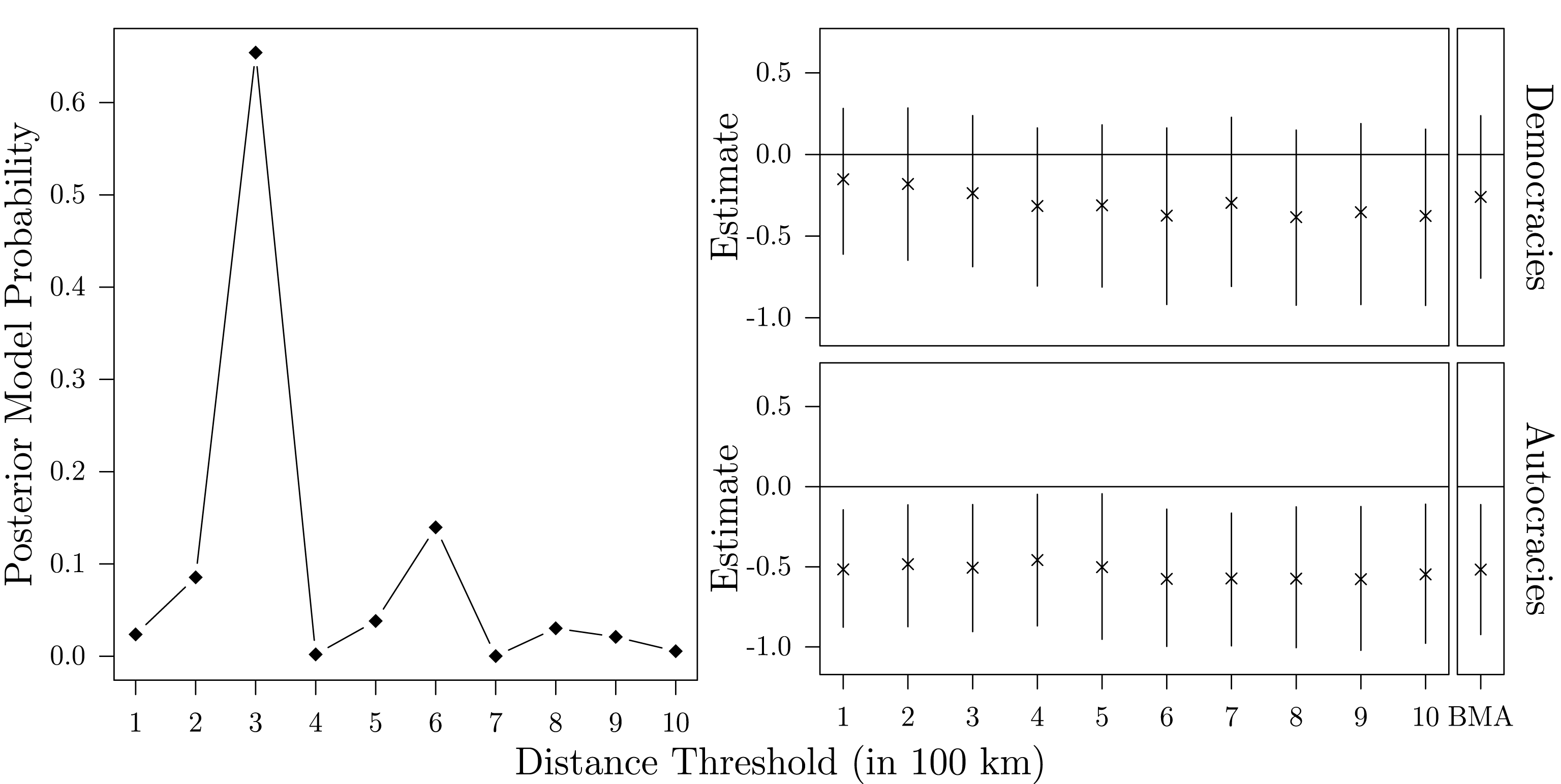
Figure 6. Spatial parameter estimates of the proportion of neighboring democracies for different neighborhood criteria (BMA).
In order to perform BMA, I specify ten different neighborhood networks using the thresholds from 100 km to 1,000 km in steps of 100 km and assign a prior probability of 0.1 to each of them. Notice that, in contrast to the semiparametric approach, these matrices take on a value of 1 if a neighboring country is located within the radius limited by a certain threshold. Hence, if two countries are connected by $\boldsymbol{W}$
with a threshold of 400 km, they also receive a value of 1 for all matrices with thresholds larger than 400 km. Again, I follow the original study and row-standardize all connectivity matrices. As the left part of Figure 6 shows, the
$\boldsymbol{W}$
with a threshold of 400 km, they also receive a value of 1 for all matrices with thresholds larger than 400 km. Again, I follow the original study and row-standardize all connectivity matrices. As the left part of Figure 6 shows, the $\boldsymbol{W}$
with a threshold of 300 km is most supported by the data. The posterior model probability for this network is 65.42% while it is only 13.97% for the second best network (600 km threshold). Yet, all ten network specifications do not notably differ in terms of the estimated spatial parameter, as the right part of Figure 6 illustrates. As Gleditsch and Ward (Reference Gleditsch and Ward2006) report, and in contrast to the conclusion obtained with the semiparametric approach, the proportion of neighboring democracies negatively affects the probability that an autocratic regime will endure while it has no effect for democracies. The same holds for the effect of a neighboring country’s transition to democracy.Footnote
19
Moreover, the predicted probability for a democratic transition is almost not affected by the specific neighborhood definition employed.Footnote
20
$\boldsymbol{W}$
with a threshold of 300 km is most supported by the data. The posterior model probability for this network is 65.42% while it is only 13.97% for the second best network (600 km threshold). Yet, all ten network specifications do not notably differ in terms of the estimated spatial parameter, as the right part of Figure 6 illustrates. As Gleditsch and Ward (Reference Gleditsch and Ward2006) report, and in contrast to the conclusion obtained with the semiparametric approach, the proportion of neighboring democracies negatively affects the probability that an autocratic regime will endure while it has no effect for democracies. The same holds for the effect of a neighboring country’s transition to democracy.Footnote
19
Moreover, the predicted probability for a democratic transition is almost not affected by the specific neighborhood definition employed.Footnote
20
In contrast to the semiparametric approach, BMA supports the conclusion about spatial spillover effects reached by Gleditsch and Ward (Reference Gleditsch and Ward2006). At the same time, it accurately accounts for network uncertainty in the estimates.
6.2 Application II: international capital tax rate competition
Located in the field of International Political Economy, the second example investigates uncertainty in the functional form of $\boldsymbol{W}$
. Although the original study was conducted by Hays (Reference Hays2003, Reference Hays2009), I reanalyze its replication by Plümper and Neumayer (Reference Plümper and Neumayer2010) who demonstrate how small and theoretically reasonable changes in the specification of the original model lead to considerable differences in the estimates of the spatial parameter. By replicating this study, I aim to exemplify how BMA performs in a situation where it has been shown that model specification issues dramatically change the parameter estimates.
$\boldsymbol{W}$
. Although the original study was conducted by Hays (Reference Hays2003, Reference Hays2009), I reanalyze its replication by Plümper and Neumayer (Reference Plümper and Neumayer2010) who demonstrate how small and theoretically reasonable changes in the specification of the original model lead to considerable differences in the estimates of the spatial parameter. By replicating this study, I aim to exemplify how BMA performs in a situation where it has been shown that model specification issues dramatically change the parameter estimates.
In the original analysis, Hays (Reference Hays2003, Reference Hays2009) studies the effective capital tax rates of twenty OECD countries with a model similar to the one shown in Equation (1) plus an additional first-order temporally lagged dependent variable. In order to show how sensitive the estimate of the spatial parameter is to small and theoretically reasonable changes in the specification of the original model, Plümper and Neumayer (Reference Plümper and Neumayer2010) estimate nine alternative model specifications (Model 2 to Model 10 in Plümper and Neumayer (Reference Plümper and Neumayer2010)). These models differ in whether or not they include (i) a temporally lagged dependent variable, (ii) unit and period fixed effects, (iii) whether or not $\boldsymbol{W}$
is row-standardized, and (iv) in the weighting scheme of
$\boldsymbol{W}$
is row-standardized, and (iv) in the weighting scheme of $\boldsymbol{W}$
.Footnote
21
Hence, the authors do not limit their attention to network uncertainty but investigate a broader range of model uncertainty. Since the focus here is on network uncertainty as a specific case of model uncertainty, the bold symbols in Figure 7 facilitate the comparison of the estimates across different network specifications by indicating the models that only differ in
$\boldsymbol{W}$
.Footnote
21
Hence, the authors do not limit their attention to network uncertainty but investigate a broader range of model uncertainty. Since the focus here is on network uncertainty as a specific case of model uncertainty, the bold symbols in Figure 7 facilitate the comparison of the estimates across different network specifications by indicating the models that only differ in $\boldsymbol{W}$
.
$\boldsymbol{W}$
.
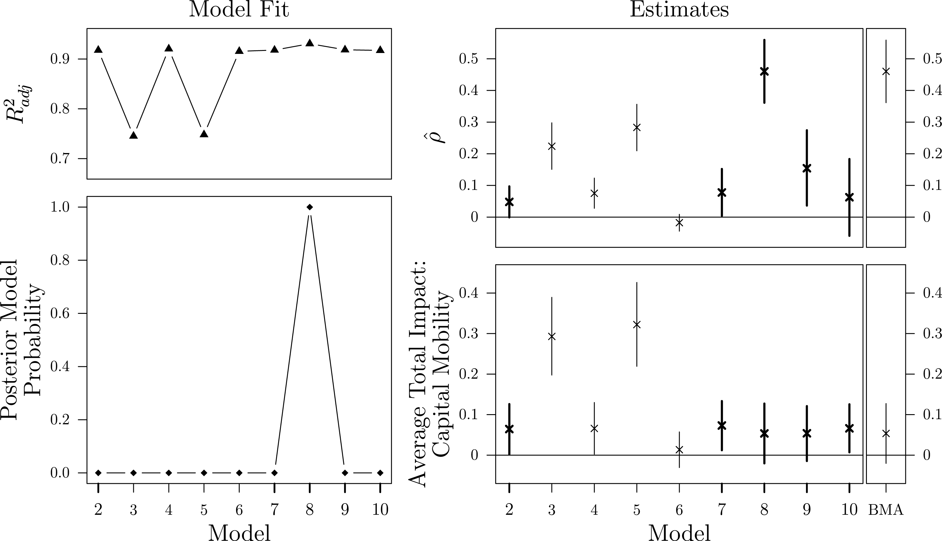
Figure 7. Adjusted $R^{2}$
, posterior model probabilities, normalized spatial parameter estimates, and average total impacts of capital mobility for different model specifications.
$R^{2}$
, posterior model probabilities, normalized spatial parameter estimates, and average total impacts of capital mobility for different model specifications.
In order to compare the estimates across models with different weighting schemes, I apply the min–max normalization. As also shown by Plümper and Neumayer (Reference Plümper and Neumayer2010), the upper right part of Figure 7 illustrates that changes in model specification have a considerable impact on the estimated spatial parameter $\hat{\unicode[STIX]{x1D70C}}$
. The size and even the sign of the estimate vary widely across the model specifications. Based on Model 6, for example, the probability that the estimate is negative is 90.3%. There is also considerable variation in
$\hat{\unicode[STIX]{x1D70C}}$
. The size and even the sign of the estimate vary widely across the model specifications. Based on Model 6, for example, the probability that the estimate is negative is 90.3%. There is also considerable variation in $\hat{\unicode[STIX]{x1D70C}}$
even across the models that only differ in the specification of
$\hat{\unicode[STIX]{x1D70C}}$
even across the models that only differ in the specification of $\boldsymbol{W}$
(Models 2, 7, 8, 9, and 10). What is more, as the top left panel shows, goodness-of-fit statistics like the adjusted
$\boldsymbol{W}$
(Models 2, 7, 8, 9, and 10). What is more, as the top left panel shows, goodness-of-fit statistics like the adjusted $R^{2}$
do not provide guidance to decide about the most appropriate model in this example.Footnote
22
Consequently, model selection techniques which rely on these measures, including the three-step procedure developed by Zhukov and Stewart (Reference Zhukov and Stewart2013), do not alleviate the problem of network uncertainty because they fail to eliminate candidate models. Only the two models that do not include the temporally lagged dependent variable exhibit a notably weaker fit. The obvious question, then, is what to infer about the countries’ interdependencies in capital taxation from these results?
$R^{2}$
do not provide guidance to decide about the most appropriate model in this example.Footnote
22
Consequently, model selection techniques which rely on these measures, including the three-step procedure developed by Zhukov and Stewart (Reference Zhukov and Stewart2013), do not alleviate the problem of network uncertainty because they fail to eliminate candidate models. Only the two models that do not include the temporally lagged dependent variable exhibit a notably weaker fit. The obvious question, then, is what to infer about the countries’ interdependencies in capital taxation from these results?
In a situation like this, BMA helps to evaluate the relative support for each model given the data and a set of possible model specifications. The bottom left panel in Figure 7 shows that, conditional on the model set and with equal prior probabilities for all models, the posterior model probability of Model 8 is almost 100%. Hence, BMA essentially reduces to a model selection technique in this example because the weighted average of the estimate across all model specifications considered here is almost identical to the estimate obtained from Model 8. However, differences in $\hat{\unicode[STIX]{x1D70C}}$
do not imply differences in the substantive effects (e.g., LeSage and Pace Reference LeSage and Pace2009, Reference LeSage and Pace2014). The lower right part of Figure 7 presents the average total impact of capital mobility as the main explanatory variable in the analysis.Footnote
23
Clearly, although the parameter estimates vary to a notable degree, all models, except for the models omitting temporal dynamics, estimate a similar average total impact of a one-unit change in capital mobility on capital taxation, irrespective of the pre-specified connectivity matrix.
$\hat{\unicode[STIX]{x1D70C}}$
do not imply differences in the substantive effects (e.g., LeSage and Pace Reference LeSage and Pace2009, Reference LeSage and Pace2014). The lower right part of Figure 7 presents the average total impact of capital mobility as the main explanatory variable in the analysis.Footnote
23
Clearly, although the parameter estimates vary to a notable degree, all models, except for the models omitting temporal dynamics, estimate a similar average total impact of a one-unit change in capital mobility on capital taxation, irrespective of the pre-specified connectivity matrix.
In conclusion, this replication study demonstrates that BMA identifies the model among a set of feasible alternative specifications that is most supported by the data even if classical model fit measures like the $R^{2}$
fail to unambiguously identify a single best fitting model. At the same time, and in line with the results of the second Monte Carlo study presented above, it also shows that the estimated effect of a regressor is less affected by the functional form of
$R^{2}$
fail to unambiguously identify a single best fitting model. At the same time, and in line with the results of the second Monte Carlo study presented above, it also shows that the estimated effect of a regressor is less affected by the functional form of $\boldsymbol{W}$
than commonly expected by practitioners.
$\boldsymbol{W}$
than commonly expected by practitioners.
7 Conclusion
Political scientists working in various subfields of the discipline increasingly apply spatial regression techniques. However, a prevalent concern that hampers the application of these methods is that the inferences are sensitive toward small changes in the structure of the predefined network $\boldsymbol{W}$
(e.g., Arbia and Fingleton Reference Arbia and Fingleton2008; Mueller and Loomis Reference Mueller and Loomis2010). The present study investigates the effects of a misspecification in
$\boldsymbol{W}$
(e.g., Arbia and Fingleton Reference Arbia and Fingleton2008; Mueller and Loomis Reference Mueller and Loomis2010). The present study investigates the effects of a misspecification in $\boldsymbol{W}$
and suggests BMA as a superior approach to address this concern. Two Monte Carlo experiments and two replication studies provide evidence for the benefits of BMA across a range of problems associated with the specification of
$\boldsymbol{W}$
and suggests BMA as a superior approach to address this concern. Two Monte Carlo experiments and two replication studies provide evidence for the benefits of BMA across a range of problems associated with the specification of $\boldsymbol{W}$
typically encountered in different subfields.
$\boldsymbol{W}$
typically encountered in different subfields.
The results challenge the notion that network uncertainty considerably distort substantive inferences. While uncertainty in the neighborhood definition can lead to biased effect estimates when $\boldsymbol{W}$
is severely misspecified and the cross-sectional dependence is strong, uncertainty about the functional form or the weighting scheme of
$\boldsymbol{W}$
is severely misspecified and the cross-sectional dependence is strong, uncertainty about the functional form or the weighting scheme of $\boldsymbol{W}$
only causes major differences in the spatial parameter estimates but not in the substantive effect estimates. Moreover, the results show that, whereas alternative techniques feature several notable deficits, BMA assesses the relative support for each of the alternative specifications and allows researchers to account for network uncertainty by conditioning the estimates on a set of theoretically plausible network structures. The simulation studies show that it correctly identifies the true underlying network and provides accurate effect estimates even without prior information about the likelihood of each network within the feasible set. Further advantages of BMA are its high flexibility, the ease of implementation, its applicability to non-nested model structures, and its coherent framework for statistical inference. Therefore, BMA is superior to alternative approaches that primarily focus on network selection or estimation.
$\boldsymbol{W}$
only causes major differences in the spatial parameter estimates but not in the substantive effect estimates. Moreover, the results show that, whereas alternative techniques feature several notable deficits, BMA assesses the relative support for each of the alternative specifications and allows researchers to account for network uncertainty by conditioning the estimates on a set of theoretically plausible network structures. The simulation studies show that it correctly identifies the true underlying network and provides accurate effect estimates even without prior information about the likelihood of each network within the feasible set. Further advantages of BMA are its high flexibility, the ease of implementation, its applicability to non-nested model structures, and its coherent framework for statistical inference. Therefore, BMA is superior to alternative approaches that primarily focus on network selection or estimation.
At the same time, it is important to emphasize that BMA is by no means a surrogate for the theoretically motivated specification of $\boldsymbol{W}$
. Ideally, theory would unambiguously determine the correct specification of
$\boldsymbol{W}$
. Ideally, theory would unambiguously determine the correct specification of $\boldsymbol{W}$
. Despite the indubitable appeal of this ideal situation, it seems more than questionable that our theories of spatial dependence will ever be able to meet this desire and convincingly produce such detailed predictions necessary to unequivocally specify the underlying network. The identification of a finite set of possible network structures is perhaps the best we can ask from our theories.
$\boldsymbol{W}$
. Despite the indubitable appeal of this ideal situation, it seems more than questionable that our theories of spatial dependence will ever be able to meet this desire and convincingly produce such detailed predictions necessary to unequivocally specify the underlying network. The identification of a finite set of possible network structures is perhaps the best we can ask from our theories.
The discussion of specification issues in $\boldsymbol{W}$
presented here focuses on the SAR model as the most popular class of spatial regression models and on the most common forms of network uncertainty encountered by political scientists. Therefore, it is by no means exhaustive. Subsequent work might investigate the consequences of network uncertainty and the utility of BMA in the context of other dependence structures like the more general spatial Durbin model, which allows for spatial dependence not only in the dependent variable but also in the regressors and the disturbances (e.g., LeSage and Pace Reference LeSage and Pace2009).
$\boldsymbol{W}$
presented here focuses on the SAR model as the most popular class of spatial regression models and on the most common forms of network uncertainty encountered by political scientists. Therefore, it is by no means exhaustive. Subsequent work might investigate the consequences of network uncertainty and the utility of BMA in the context of other dependence structures like the more general spatial Durbin model, which allows for spatial dependence not only in the dependent variable but also in the regressors and the disturbances (e.g., LeSage and Pace Reference LeSage and Pace2009).
In the absence of sufficient theoretical guidance on the precise network structure, BMA complements the empirical analysis of interdependencies by conditioning the parameter estimates on a set of feasible network structures instead of a single network typology. As such, BMA is a powerful and easily implementable approach to ameliorate the haphazard specification of $\boldsymbol{W}$
in the face of insufficient theoretical guidance.
$\boldsymbol{W}$
in the face of insufficient theoretical guidance.
Supplementary material
For supplementary material accompanying this paper, please visit https://doi.org/10.1017/pan.2019.12.


 Open access