


1. Introduction
Let $({{\mathrm M}},\,g)$ be a Riemannian manifold, denote by $\nabla ^{g}$
 its Levi Civita connection, and consider a non-vanishing $3$
 -form $H\in \Omega ^{3}({{\mathrm M}})$
 . The Bismut connection associated with the pair $(g,\,H)$
 is defined via the identity

for all $X,\,Y,\,Z\in \Gamma (T{{\mathrm M}})$ , it is the unique metric connection on ${{\mathrm M}}$
 with totally skew-symmetric torsion $H$
 , and it has the same geodesics as $\nabla ^{g}$
 .
.
These connections were successfully used in index theory problems in complex non-Kähler geometry [Reference Bismut7], where they are characterized as the only complex metric connections with totally skew-symmetric torsion $H=d^{c}\omega$ on a given Hermitian manifold $({{\mathrm M}},\,g,\,J)$
 , see e.g. [Reference Gauduchon16]. In this setting, strong Kähler with torsion (SKT) complex manifolds are precisely the Hermitian manifolds $({{\mathrm M}},\,g,\,J)$
 whose Kähler form $\omega$
 satisfies the condition $dd^{c}\omega =0$
 , or, equally, whose Bismut connection has closed torsion, see for instance the survey [Reference Fino and Tomassini11] for more details. On the other hand, the class of Riemannian manifolds admitting a Bismut connection $\nabla$
 whose torsion $H$
 is $\nabla$
 -parallel has been throughly studied in the literature, as this condition naturally holds for several geometrically significant structures as naturally reductive spaces, nearly Kähler and Sasakian structures among others, see e.g. [Reference Agricola1, Reference Agricola, Ferreira and Friedrich2, Reference Cleyton, Moroianu and Semmelmann10]. Furthermore, Bismut connections are also of interest in theoretical and mathematical physics, see [Reference Friedrich and Ivanov12] and the references therein for a detailed explanation.
Bismut connections with closed torsion form play a central role in generalized Riemannian geometry, where they are naturally associated with generalized metrics on exact Courant algebroids, see [Reference Garcia-Fernández13, Reference Garcia-Fernández and Streets15]. In this case, since the torsion of $\nabla$ is non-vanishing, the Ricci tensor ${{\rm Ric}}^{\nabla }$
 is not symmetric, and one has (see [Reference Garcia-Fernández and Streets15, Prop. 3.18])
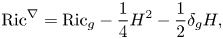
where ${{\rm Ric}}_g$ denotes the Ricci tensor of $\nabla ^{g}$
 , $\delta _g$
 is the formal adjoint of $d$
 , and the symmetric 2-tensor $H^{2}$
 is defined as $H^{2}(X,\,Y) := g(\imath _XH,\,\imath _YH)$
 , for every $X,\,Y\in \Gamma (T{{\mathrm M}})$
 .
.
It is clear from (1.1) that a Bismut connection $\nabla$ with closed torsion form $H$
 is Ricci flat, i.e., ${{\rm Ric}}^{\nabla }=0$
 , if and only if $H$
 is a $g$
 -harmonic $3$
 -form and the Ricci tensor of $g$
 satisfies the equation ${{\rm Ric}}_g = \frac 14 H^{2}$
 . A pair $(g,\,H)$
 with $dH=0$
 and giving rise to a Ricci flat Bismut connection $\nabla$
 is called a Bismut Ricci flat pair (BRF pair for short) throughout the following. In generalized Riemannian geometry, such pairs correspond to special types of generalized Einstein structures, see [Reference Garcia-Fernández and Streets15, Ch. 3] for more information. We recall here that for a BRF pair $(g,\,H)$
 the scalar curvature ${{\rm Scal}}_g$
 and the norm of $H,$
 which are related by the identity ${{\rm Scal}}_g = \frac 14 ||H||^{2}$
 , are constant on ${{\mathrm M}}$
 , see [Reference Lee18, lemma 2.24].
BRF pairs are fixed points of the generalized Ricci flow, a geometric flow introduced in [Reference Callan, Friedan, Martinec and Perry8, Reference Oliynyk, Suneeta and Woolgar19] in the context of renormalization group flows of two-dimensional nonlinear sigma models. To describe this flow, consider a family of Riemannian metrics $g_t$ depending on a real parameter $t$
 , fix a closed $3$
 -form $H_0\in \Omega ^{3}({{\mathrm M}})$
 and let $H_t = H_0 + db_t$
 , where $b_t\in \Omega ^{2}({{\mathrm M}})$
 . Then, the generalized Ricci flow for $(g_t,\,b_t)$
 is defined as follows
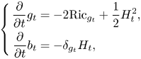
and it is well-posed on compact manifolds, see e.g. [Reference Garcia-Fernández and Streets15]. Notice that BRF pairs can also be regarded as trivial examples of steady solitons for the generalized Ricci flow. Indeed, the latter are defined by pairs $(g,\,H)$ satisfying the more general equations
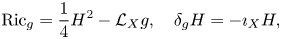
for some vector field $X\in \Gamma (T{{\mathrm M}})$ . The existence of non-trivial solitons on compact (complex) $4$
 -manifolds has been recently proved in [Reference Streets23, Reference Streets and Ustinovskiy27].
Remarkably, the flow (1.2) can be seen as a generalization of Hamilton's Ricci flow to Bismut connections with closed torsion form [Reference Streets20] and as a flow of generalized metrics on exact Courant algebroids [Reference Garcia-Fernández13, Reference Streets21]. Moreover, it is related to some geometric flows in Hermitian Geometry, like the pluriclosed flow and the generalized Kähler Ricci flow, see e.g. [Reference Garcia-Fernández, Jordan and Streets14, Reference Streets22, Reference Streets and Tian24–Reference Streets and Tian26]. The reader may refer to the recent book [Reference Garcia-Fernández and Streets15] for an excellent introduction to the topic.
Standard examples of manifolds carrying BRF pairs are provided by compact simple Lie groups endowed with the bi-invariant metric (given by the negative of the Cartan–Killing form) and the standard harmonic $3$ -form, see e.g. [Reference Garcia-Fernández and Streets15, Prop. 3.53]. Notice that, in such a case, the corresponding Bismut connection is flat. On the other hand, a simply connected compact Riemannian manifold admitting a flat Bismut connection is isometric to a product of compact simple Lie groups with bi-invariant metrics [Reference Garcia-Fernández and Streets15, Thm. 3.54]. It is currently not known whether other left-invariant BRF pairs may exist on compact Lie groups.
Since in the Riemannian case every homogeneous Ricci flat manifold is flat [Reference Alekseevsky and Kimelfeld4], M. Garcia-Fernández and J. Streets asked the following:
Question ([Reference Garcia-Fernández and Streets15])
Given $({{\mathrm M}},\,g,\,H)$ a homogeneous Riemannian manifold with $H$
 invariant and zero Bismut Ricci curvature, is the associated Bismut connection flat?
In this paper, we answer this question negatively. After showing some general facts on compact homogeneous spaces with non-zero third Betti number in § 2, we examine low dimensional compact homogeneous spaces in § 3. Since the $3$ - and $4$
 -dimensional case are well understood from the results of [Reference Garcia-Fernández and Streets15], we focus on $5$
 -dimensional compact homogeneous spaces and we obtain a full classification of those admitting invariant BRF pairs in theorem 3.2. Beyond the case of compact Lie groups, we find a family of compact homogeneous spaces ${{\mathrm M}}_{p,q}$
 parametrized by a pair of positive integers $p\geq q$
 with $\mathrm {gcd}(p,\,q)=1$
 , all diffeomorphic to $S^{3}\times S^{2}$
 , where we prove the existence of invariant BRF pairs $(g,\,H)$
 for which the corresponding Bismut connection $\nabla$
 is not flat, the metric $g$
 is not Einstein and the torsion form $H$
 is not $\nabla$
 -parallel, see theorem 3.3. The uniqueness of such pairs is also studied in the same theorem. Finally, in § 4, we investigate the behaviour of the homogeneous generalized Ricci flow on the spaces ${{\mathrm M}}_{p,q}$
 with $p\neq q$
 , showing that the invariant BRF pairs found in theorem 3.3 are global attractors, see theorem 4.1.
As an additional remark, in § 3.1 we show that our examples are particular cases of a general construction by Kobayashi in the Riemannian Einstein setting [Reference Kobayashi17], and we pave the way for a possible use of his construction to provide new examples of generalized Einstein manifolds, see proposition 3.7.
Notation. Throughout the paper, Lie groups will be denoted by capital letters and their Lie algebras will be denoted by the respective gothic letters. The Cartan–Killing form of a Lie algebra will be always denoted by $B$ . When a Lie group ${{\mathrm G}}$
 acts on a manifold ${{\mathrm M}}$
 , the vector field associated to any $X\in \mathfrak {g}$
 will be denoted by $\hat X$
 . Finally, the space of Riemannian metrics on a manifold ${{\mathrm M}}$
 will be denoted by $\mathcal {M}({{\mathrm M}})$
 .
.
2. Compact homogeneous spaces with positive third Betti number
A preliminary step in the search for invariant Bismut Ricci flat connections on compact homogeneous spaces consists in finding conditions under which the third Betti number of the space is positive.
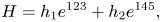
A typical example is given by compact semisimple Lie groups, where $b_3$ coincides with the number of simple factors, see [Reference Chevalley and Eilenberg9]. In particular, when ${{\mathrm G}}$
 is a compact simple Lie group, then the third cohomology group $H^{3}({{\mathrm G}},\,\mathbb {R})$
 is generated by the standard $3$
 -form $\omega$
 defined as follows
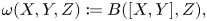
for every left-invariant vector fields $X,\,Y,\,Z$ on ${{\mathrm G}}$
 . More generally, in [Reference Azad3] it was proved that the isotropy subgroup ${{\mathrm K}}$
 of a compact homogeneous space ${{\mathrm M}}={{\mathrm G}}/{{\mathrm K}}$
 such that $b_3({{\mathrm M}}) \geq 1$
 must be finite whenever ${{\mathrm G}}$
 is simple. In the next theorem, we review this result and we obtain some new restrictions on ${{\mathrm K}}$
 in the case where ${{\mathrm G}}$
 is locally a product of two simple factors.
Theorem 2.1 Let ${{\mathrm G}}$ be a compact Lie group and let ${{\mathrm M}}={{\mathrm G}}/{{\mathrm K}}$
 be a ${{\mathrm G}}$
 -homogeneous space with $b_3({{\mathrm M}})\geq 1$
 . Then
(a) if ${{\mathrm G}}$
 is simple, then ${{\mathrm K}}$ is finite;
(b) if ${{\mathrm G}}$
is locally a product of two simple factors ${{\mathrm G}}_1,\,{{\mathrm G}}_2$, then either the Lie algebra $\mathfrak {k}$ is contained in one of the two factors $\frak g_i$ or the Lie algebras $\frak g_i$ contain subalgebras $\mathfrak {k}_i$ isomorphic to $\mathfrak {k}$ and the projections $p_i:\mathfrak {k}\to \frak g_i$ are isomorphisms onto $\mathfrak {k}_i,$ for $i=1,\,2$.


Proof. The assertion (a) was proved in [Reference Azad3]. We review the proof here. Let $\pi :{{\mathrm G}}\to {{\mathrm G}}/{{\mathrm K}}$ be the projection and consider a closed $3$
 -form $\phi$
 on ${{\mathrm M}}$
 . As ${{\mathrm G}}$
 is compact, we can suppose that $\phi$
 is ${{\mathrm G}}$
 -invariant. If $\hat \phi \in \Omega ^{3}({{\mathrm G}})$
 is the closed $3$
 -form $\pi ^{*}(\phi )$
 , then $\hat \phi$
 is invariant under left ${{\mathrm G}}$
 -translations and right ${{\mathrm K}}$
 -translations. Since ${{\mathrm G}}$
 is simple, the third cohomology group $H^{3}({{\mathrm G}},\,\mathbb {R})$
 is generated by the standard $3$
 -form $\omega$
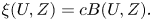
 defined in (2.1). Thus, $\hat \phi = c\,\omega + d\xi$
 , for some $c\in {{\mathbb {R}}}$
 and some $2$
 -form $\xi \in \Omega ^{2}({{\mathrm G}})$
 . Again by compactness, we can suppose that $\xi$
 is invariant under left ${{\mathrm G}}$
 -translations and right ${{\mathrm K}}$
 -translations. This implies that, given $X,\,Y\in \frak g$
 and $Z\in \mathfrak {k}$
 , we have

where we see $\xi$ as an element of $\Lambda ^{2}(\frak g^{*})$
 . Moreover, $\imath _Z\hat \phi =0$
 , so that

Hence

As ${{\mathrm G}}$ is simple, we have $\frak g= [\frak g,\,\frak g]$
 and therefore for every $U\in \frak g$
Suppose now $\frak k\neq \{0\}$ and choose a non-zero element $Z\in \frak k$
 . By (2.2) we have that $0=c B(Z,\,Z)$
 , hence $c=0$
 and $\imath _{\frak k}\xi =0$
 . This means that $\xi$
 descends to a $2$
 -form on ${{\mathrm M}}$
 with $d\xi =\phi$
 . Consequently, every element in $H^{3}({{\mathrm M}},\,\mathbb {R})$
 must be trivial, a contradiction.
We now prove (b). Using the same notation as in (a), suppose $0\neq [\phi ]\in H^{3}({{\mathrm M}},\,\mathbb {R})$ and consider the corresponding $3$
 -form $\hat \phi \in \Omega ^{3}({{\mathrm G}})$
 . The form $\hat \phi$
 can be written as $\hat \phi = c_1\,\omega _1 + c_2\,\omega _2 + d\xi$
 , where $\omega _i$
 is the standard $3$
 -form on ${{\mathrm G}}_i$
 , for $i=1,\,2$
 . If $Z\in \mathfrak {k}$
 , then for every $X,\,Y\in \mathfrak {g}$

Hence

where $B_i$ is the Cartan–Killing forms on $\frak g_i$
 , and the subscript ${-}_i$
 denotes the projection along the $i^{th}$
 -component $\frak g_i$
 . Now, suppose that, say, $p_1$
 has a non-trivial kernel containing some $Z\neq 0$
 such that $Z_1=0$
 and $Z_2\neq 0$
 . As ${{\mathrm G}}$
 is semisimple, we can express $Z = \sum _k[X_k,\,Y_k]$
 for some vectors $X_k,\,Y_k\in \frak g$
 . Hence,

forcing $c_2=0$ . If $c_1=0$
 , then $\hat \phi = d\xi$
 and $\imath _{\mathfrak {k}}\xi = 0$
 , so that $\xi$
 descends to an invariant $2$
 -form on ${{\mathrm M}}$
 and $\phi$
 is exact, a contradiction. Therefore $c_1\neq 0$
 , and for every $Z'\in \mathfrak {k}$
 we have $0=\xi (Z',\,Z') = c_1B_1(Z'_1,\,Z'_1)$
 so that $Z'_1=0$
 , implying $\mathfrak {k}\subseteq \frak g_2$
 .
.
Remark 2.2 Note that if a projection, say $p_1$ , is also surjective, namely $\mathfrak {k}_1=\mathfrak {g}_1$
 , then ${{\mathrm M}}$
 is diffeomorphic to the simple factor ${{\mathrm G}}_2$
 (up to a covering).
3. Compact homogeneous spaces with invariant BRF pairs
In this section, we investigate the existence of compact homogeneous spaces admitting invariant pairs $(g,\,H)$ such that the corresponding Bismut connection $\nabla = \nabla ^{g} + \frac 12 g^{-1}H$
 is Ricci flat and non-flat, and we aim at understanding whether the generalized Alekseevsky–Kimelfeld theorem may hold, i.e., whether the Bismut connection induced by an invariant BRF pair on a homogeneous space must be necessarily flat.
Basic examples of such spaces are given by compact (semi)simple Lie groups endowed with a bi-invariant metric $g$ and the standard harmonic $3$
 -form $\omega$
 . In these cases, the associated Bismut connection is flat. Particular examples are given by the standard $3$
 -sphere $S^{3}\cong {{\mathrm {SU}}}(2)$
 endowed with a constant curvature metric, and the product ${{\mathrm M}}=S^{3}\times S^{1}$
 with the product metric and the standard $3$
 -form on $S^{3}$
 viewed as a $3$
 -form on ${{\mathrm M}}$
 (cf. [Reference Garcia-Fernández and Streets15, Ex. 3.57]).
The $3$ -dimensional case is settled in [Reference Garcia-Fernández and Streets15, Prop. 3.55], where it is proved that the existence of a BRF pair $(g,\,H)$
 on a $3$
 -manifold ${{\mathrm M}}^{3}$
 implies that $({{\mathrm M}}^{3},\,g)$
 has constant sectional curvature and the associated Bismut connection is flat. The $4$
 -dimensional case can be completely understood following the reasoning in the proof of [Reference Garcia-Fernández and Streets15, Thm. 8.26]. We specify it here for the reader's convenience.Footnote 1
Proposition 3.1 Let ${{\mathrm M}}^{4}$ be a $4$
 -dimensional compact manifold admitting a BRF pair $(g,\,H)$
 . Then, the associated Bismut connection is flat.
Proof. As the $3$ -form $H$
 is harmonic, the $1$
 -form $\theta := *_gH$
 is also harmonic. Therefore, by Bochner formula, we have
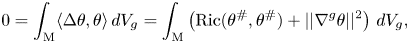
so that $\theta$ is parallel and $0={{{\rm Ric}}}(\theta ^\#,\,\theta ^\#)=\frac 14 H^{2}(\theta ^\#,\,\theta ^\#) = \frac 14 ||\imath _{\theta ^{\sharp }}H||^{2}$
 . This implies that the universal cover of ${{\mathrm M}}^{4}$
 splits isometrically as a product $\mathrm {N}^{3}\times \mathbb {R}$
 , for some $3$
 -dimensional space $\mathrm {N}^{3}$
 , and that $\imath _vH=0$
 whenever $v$
 is tangent to the flat factor. The claim now follows from the $3$
 -dimensional case.
We now turn to the $5$ -dimensional case and in the next theorem we determine which $5$
 -dimensional compact homogeneous spaces may admit invariant BRF pairs.
Theorem 3.2 Let $({{\mathrm M}},\,g)$ be a compact $5$
 -dimensional homogeneous Riemannian manifold. If ${{\mathrm M}}$
 admits a harmonic $3$
 -form $H$
 such that $(g,\,H)$
 is a BRF pair, then one of the following holds:
(i) ${{\mathrm M}}$
is finitely covered by a compact Lie group;(ii) ${{\mathrm M}}$
is finitely covered by ${{\mathrm {SU}}}(2)^{2}/{{\mathbb {T}}}^{1}$, where ${{\mathbb {T}}}^{1}$ is embedded diagonally into ${{\mathrm {SU}}}(2)^{2}$.


Proof. We consider the compact Lie group ${{\mathrm G}}$ given by the connected full isometry group of $({{\mathrm M}},\,g)$
 , and we recall that any harmonic form is invariant under the ${{\mathrm G}}$
 -action. We start noting that we can assume $H\neq 0$
 , as otherwise by [Reference Alekseevsky and Kimelfeld4] the Ricci flat metric $g$
 would be flat and ${{\mathrm M}}$
 would be covered by a torus.
We first study the case where ${{\mathrm G}}$ is semisimple. Let ${{\mathrm K}}$
 denote the isotropy group of the ${{\mathrm G}}$
 -action on ${{\mathrm M}}$
 at a fixed point $p$
 . Then, $\dim {{\mathrm K}}$
 belongs to the set $\{1,\,2,\,3,\,4,\,5,\,6\}$
 . Indeed, the isotropy representation embeds ${{\mathrm K}}$
 into ${{\mathrm {SO}}}(5)$
 and ${{\mathrm K}}$
 is a proper subgroup, as the standard representation of ${{\mathrm {SO}}}(5)$
 has no non-trivial invariant $3$
 -forms. Moreover, a proper subgroup of ${{\mathrm {SO}}}(5)$
 has dimension at most $6=\dim {{\mathrm {SO}}}(4)$
 , with equality if and only if ${{\mathrm K}}$
 is conjugate to the standard ${{\mathrm {SO}}}(4)$
 . Again, this case can be ruled out as there are no non-trivial invariant $3$
 -forms.
The case $\dim {{\mathrm K}}=5$ cannot occur, as there are no $5$
 -dimensional subgroups of ${{\mathrm {SO}}}(5)$
 (the rank is at most two: if the rank is $1$
 , then ${{\mathrm K}}\cong {{\mathbb {T}}}^{1}$
 or ${{\mathrm {SU}}}(2)$
 , if the rank is $2$
 , then either ${{\mathrm K}}\cong {{\mathbb {T}}}^{2}$
 or ${{\mathrm K}}\cong {{\mathbb {T}}}^{1}\cdot {{\mathrm {SU}}}(2)$
 , never with dimension $5$
 ).
).
If $\dim {{\mathrm K}}=4$ , then, by dimensional reasons, ${{\mathrm K}}$
 and ${{\mathrm G}}$
 are locally isomorphic to ${{\mathbb {T}}}^{1}\times {{\mathrm {SU}}}(2)$
 and ${{\mathrm {SU}}}(2)^{3}$
 , respectively. We denote by $\frak z$
 the centre of $\mathfrak {k}$
 and by $\frak k_s\cong \mathfrak {su}(2)$
 the semisimple part of $\frak k$
 . If $\mathfrak {g}=\oplus _{i=1}^{3}\mathfrak {g}_i$
 , with $\mathfrak {g}_i\cong \mathfrak {su}(2)$
 , and $p_i:\mathfrak {g}\to \mathfrak {g}_i$
 are the projections for $i=1,\,2,\,3$
 , then we may suppose that $p_1(\mathfrak {z})\neq \{0\}$
 , so that $p_1(\mathfrak {k}_s)=\{0\}$
 . Since $\mathfrak {k}_s$
 cannot coincide with $\mathfrak {g}_2$
 or $\mathfrak {g}_3$
 and since it is simple, we see that $p_i(\mathfrak {k}_s)=\mathfrak {g}_i$
 and $p_i(\mathfrak {z})=\{0\}$
 for $i=2,\,3$
 . Therefore, the manifold ${{\mathrm M}}$
 is (up to a finite covering) ${{\mathrm G}}$
 -diffeomorphic to ${{\mathrm {SU}}}(2)/{{\mathbb {T}}}^{1}\times {{\mathrm {SU}}}(2)^{2}/\Delta {{\mathrm {SU}}}(2)\cong S^{2}\times S^{3}$
 . In this case, the isotropy representation contains two inequivalent modules and therefore the above diffeomorphism maps the metric $g$
 to a product metric. As the $3$
 -form $H$
 on $S^{2}\times S^{3}$
 is the pull-back of a $3$
 -form on the $S^{3}$
 -factor, we see that the Ricci tensor on the $S^{2}$
 -factor should vanish, a contradiction.
If $\dim {{\mathrm K}} = 3$ , then $\dim {{\mathrm G}}= 8$
 and, being semisimple, this implies ${{\mathrm G}}\cong {{\mathrm {SU}}}(3)$
 , which is simple. This contradicts theorem 2.1.
The case $\dim {{\mathrm K}} = 2$ can be ruled out as there are no semisimple groups of dimension $7$
 . The last case $\dim {{\mathrm K}} = 1$
 forces ${{\mathrm G}}\cong {{\mathrm {SU}}}(2)^{2}$
 and theorem 2.1 says that ${{\mathrm K}}$
 is embedded diagonally into ${{\mathrm G}}$
 , unless $\mathfrak {k}$
 is contained in one of the factors $\mathfrak {su}(2)$
 . When this occurs, ${{\mathrm M}}$
 is ${{\mathrm G}}$
 -diffeomorphic (up to a covering) to ${{\mathrm {SU}}}(2)\times S^{2}$
 . As the isotropy $\mathfrak {k}$
 acts on the tangent space of $S^{2}$
 with no non-zero invariant vector and trivially on the tangent space of ${{\mathrm {SU}}}(2)$
 , we see that the above splitting is isometric. Moreover, an invariant $3$
 -form $H$
 on ${{\mathrm M}}$
 is of the form $H_1+H_2$
 , where $H_1$
 is an invariant form on ${{\mathrm {SU}}}(2)$
 , while $H_2 = \theta \wedge \sigma$
 , where $\theta$
 is any invariant $1$
 -form on ${{\mathrm {SU}}}(2)$
 and $\sigma$
 is the volume form of $S^{2}$
 . As $dH_2=d\theta \wedge \sigma$
 and $dH_1\in \Lambda ^{3}(\mathfrak {su}(2))$
 , we see that $dH=0$
 forces $H=H_1$
 . This means that $\imath _vH=0$
 for every vector $v$
 tangent to the $S^{2}$
 factor, implying that ${{\rm Ric}}_{S^{2}}\equiv 0$
 , a contradiction.
We now deal with the non-semisimple case. Let ${{\mathrm Z}}$ be the connected centre of ${{\mathrm G}}$
 and let ${{\mathrm L}}$
 be the semisimple part of ${{\mathrm G}}$
 , which is a compact normal subgroup. We first summarize some basic observations:
(1) all ${{\mathrm L}}$
-orbits are diffeomorphic. Indeed, ${{\mathrm L}}$ is a normal subgroup of ${{\mathrm G}}$, so for every $p\in {{\mathrm M}}$ and $g\in {{\mathrm G}}$ we have ${{\mathrm L}}\cdot gp=g({{\mathrm L}}\cdot p)$. A generic ${{\mathrm L}}$-orbit will be denoted by $\mathcal {O}$;(2) let ${{\mathrm U}} := \{ z\in {{\mathrm Z}} {\ |\ }z({{\mathrm L}}\cdot p) = {{\mathrm L}}\cdot p,\,~\forall p\in {{\mathrm M}}\}$
. Then, ${{\mathrm U}}$ is a closed subgroup of the torus ${{\mathrm Z}}$ and we can find a closed subgroup ${{\mathrm Z}}_1\subseteq {{\mathrm Z}}$ with ${{\mathrm Z}}_1\cap {{\mathrm U}}=\{e\}$, ${{\mathrm Z}} = {{\mathrm U}}\cdot {{\mathrm Z}}_1$ and ${{\mathrm L}}\cdot {{\mathrm Z}}_1$ acting transitively on ${{\mathrm M}}$. Indeed, at each point $q\in {{\mathrm M}}$ we have that $T_q{{\mathrm M}} = T_q({{\mathrm Z}}_1\cdot q) \oplus T_q({{\mathrm L}}\cdot q)$. In detail, if $X\in \mathfrak {z}_1$ with $\hat X_q\in T_q({{\mathrm L}}\cdot q)$, then for every $g\in {{\mathrm G}}$ we have $\hat X_{gq}= g_*\hat X_q\in T_{gq}({{\mathrm L}}\cdot gq)$, meaning that $X\in \mathfrak {u}$, whence $X=0$;(3) the manifold ${{\mathrm M}}$
is ${{\mathrm G}}$-diffeomorphic (up to a finite covering) to the product ${{\mathrm Z}}_1\times \mathcal {O}$. Indeed, the map $F : {{\mathrm Z}}_1\times \mathcal {O}\to {{\mathrm M}}$ given by $F(z,\,p)=z\cdot p$ is a local diffeomorphism, hence a covering thanks to the compactness of the involved spaces.


Since ${{\mathrm L}}$ is non-trivial, its orbits have dimension at least $2$
 , whence $\dim {{\mathrm Z}}_1 = {\mathrm {chm}}({{\mathrm M}},\,{{\mathrm L}})\leq 3$
 . We now proceed by looking at the possible dimensions of ${{\mathrm Z}}_1$
 :
:
(a) $\dim {{\mathrm Z}}_1 = 1$
. The generic ${{\mathrm L}}$-orbit $\mathcal {O}$ has dimension $4$ and, up to a finite covering, it is ${{\mathrm L}}$-diffeomorphic to ${{\mathrm {SO}}}(5)/{{\mathrm {SO}}}(4)$, ${{\mathrm {SU}}}(3)/\mathrm {S}({{\mathrm U}}(1){{\mathrm U}}(2))$ or ${{\mathrm {SO}}}(4)/{{\mathbb {T}}}^{2}$ (cf. [Reference Bérard-Bergery5]). As the isotropy representation has no non-trivial invariant vector in the tangent space of $\mathcal {O}$, we see that the splitting in (3) is isometric. As the space of invariant $3$-forms on $\mathcal {O}$ is trivial, the form $H$ is given by $H=dt\wedge \sigma$, where $dt\in \Lambda ^{1}({{\mathbb {T}}}^{1})^{{{\mathbb {T}}}^{1}}$ and $\sigma$ is an ${{\mathrm L}}$-invariant $2$-form. Then, ${{\rm Ric}}_g(\partial _t,\,\partial _t)=0$, while $||\imath _{\partial _t}H||^{2} \neq 0$, a contradiction;(b) $\dim {{\mathrm Z}}_1=2$
. In this case, $\dim \mathcal {O}=3$, and ${{\mathrm L}}$ must be either ${{\mathrm {SU}}}(2)$ or ${{\mathrm {SO}}}(3)$, up to covering. In the former case, ${{\mathrm M}}$ is a Lie group up to covering; in the latter, $\mathcal {O}$ is covered by $S^{3}$ and the same argument as above shows that the splitting ${{\mathrm M}}={{\mathrm Z}}_1\times S^{3}$ is isometric. In this case, $H$ is a multiple of the volume form on the $S^{3}$ factor, as this has no non-trivial invariant $1$- or $2$-forms. Moreover, the metric splits as the product of a flat metric on ${{\mathrm Z}}_1$ and a multiple of the standard metric on $S^{3}$. Consequently, the associated Bismut connection is flat;(c) $\dim {{\mathrm Z}}_1=3$
. Here $\mathcal {O} \cong S^{2} = {{\mathrm {SU}}}(2)/{{\mathbb {T}}}^{1}$, so that the splitting (3) is isometric. The form $H$ can be expressed as $H=\phi \wedge \nu$, where $\phi$ is an invariant $1$-form on ${{\mathrm Z}}_1$ and $\nu$ is the volume form on $S^{2}$. Again, $||\imath _vH||^{2}\neq 0$, for every $v$ in $T{{\mathrm Z}}_1$, while ${{\rm Ric}}_g(v,\,v)=0$, a contradiction.


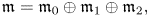
The previous result leads us to consider the homogeneous spaces ${{\mathrm M}} = ({{\mathrm {SU}}}(2)\times {{\mathrm {SU}}}(2) ) / {{\mathrm K}}$ , with ${{\mathrm K}}\cong {{\mathbb {T}}}^{1}$
 embedded diagonally. Up to an automorphism of ${{\mathrm G}} = {{\mathrm {SU}}}(2)^{2}$
 , we can suppose that ${{\mathrm K}}$
 is of the form

for some $p,\,q\in \mathbb {N}$ , with $p\geq q\geq 1$
 and $\rm {gcd}(p,\,q)=1$
 . We then let ${{\mathrm M}}_{p,q} := {{\mathrm G}}/{{\mathrm K}}_{p,q}$
 and we recall that all these homogeneous spaces are diffeomorphic to $S^{3}\times S^{2}$
 , see [Reference Wang and Ziller28, Prop. 2.3], although no explicit diffeomorphism is known (except when $p=q=1$
 ).
).
We have the following.
Theorem 3.3 The $5$ -dimensional compact homogeneous space ${{\mathrm M}}_{p,q}$
 admits a ${{\mathrm G}}$
 -invariant BRF pair $(g_o,\,H_o)$
 such that the associated Bismut connection is non-flat. More precisely
• when $p\neq q,$
the space of ${{\mathrm G}}$-invariant BRF pairs $\mathcal {B}({{\mathrm M}}_{p,q})^{{\mathrm G}}$ is given by $\mathbb {R}^{+}(g_o,\,H_o);$• when $p=q=1,$
the pair $(g_o,\,H_o)$ admits a suitable neighbourhood $\mathcal {U}$ in $\mathcal {M}({{\mathrm M}}_{1,1})\times \Omega ^{3}({{\mathrm M}}_{1,1})$ such that $\mathcal {U}\cap \mathcal {B}({{\mathrm M}}_{1,1})^{{\mathrm G}}$ coincides with $\mathcal {U}\cap {{\mathbb {R}}}^{+}(g_o,\,H_o)$.


Proof. We begin observing that ${{\mathrm M}}_{p,q}$ does not admit any Bismut flat connection. Indeed, by [Reference Garcia-Fernández and Streets15, Thm. 3.54], a simply connected compact Riemannian manifold admitting a Bismut flat connection is isometric to a product of compact simple Lie groups with bi-invariant metrics. We obtain our claim by observing that there are no $5$
 -dimensional compact semisimple Lie groups.
In the Lie algebra $\mathfrak {su}(2)$ we select the elements
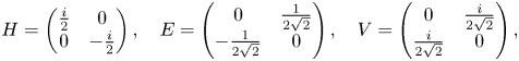
so that $[H,\,E]=V$ , $[H,\,V]=-E$
 , $[H,\,V]= -E$
 and $[E,\,V]=\frac 12 H$
 . If $B$
 denotes the Cartan–Killing form of $\mathfrak {su}(2)$
 , then $B(E,\,E)=B(V,\,V)=-1$
 , $B(H,\,H)=-2$
 . Then, we can choose the following basis of $\mathfrak {g}$
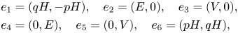
so that $\mathfrak {k}_{p,q}=\mathbb {R} e_6$ , while $\mathfrak {m}:= {\mathrm {span}_{{\mathbb {R}}}}(e_1,\,\ldots,\,e_5)$
 is an $\textrm{ad} (\mathfrak {k}_{p,q})$
 -invariant subspace and $\frak g= \mathfrak {k}_{p,q}+\mathfrak {m}$
 is an $\textrm{ad} (\mathfrak {k}_{p,q})$
 -invariant $B$
 -orthogonal decomposition. An $\textrm{ad} (\mathfrak {k}_{p,q})$
 -irreducible decomposition of $\mathfrak {m}$
 is given by
where $\mathfrak {m}_0={{\mathbb {R}}}e_1$ , $\mathfrak {m}_1= \mathrm {span}_{{\mathbb {R}}}(e_2,\,e_3)$
 and $\mathfrak {m}_2=\mathrm {span}_{{\mathbb {R}}}(e_4,\,e_5)$
 . Moreover, we have
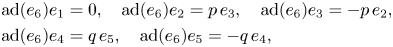
thus the module $\mathfrak {m}_0$ is trivial, while the modules $\mathfrak {m}_1$
 and $\mathfrak {m}_2$
 are non-trivial and inequivalent if $p\neq q$
 , and non-trivial and equivalent if $p=q$
 . We will discuss the cases $p\neq q$
 and $p=q$
 separately.
In the following, $\mathcal {B}^{*} = (e^{1},\,e^{2},\,e^{3},\,e^{4},\,e^{5})$ denotes the dual basis of $\mathcal {B}$
 , and the shortening $e^{ijk\cdots }$
 is used to denote the wedge product of covectors $e^{i}\wedge e^{j} \wedge e^{k} \wedge \cdots$
 . Moreover, we fix the orientation on $\mathfrak {m}$
 for which $\mathcal {B}$
 is positively oriented.
Case $\boldsymbol {p\neq q}$ . We have

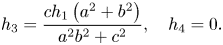
and a generic invariant 3-form is given by
for some $h_1,\,h_2\in \mathbb {R}$ . Using the Koszul formula for the differential of invariant forms on $\mathfrak {m}$

where $[X_i,\,X_j]_{\mathfrak {m}}$ denotes the projection of $[X_i,\,X_j]$
 onto $\mathfrak {m}$
 , we see that $H$
 is closed if and only if $(h_1,\,h_2) = (\lambda q,\,\lambda p)$
 , for some $\lambda \in {{\mathbb {R}}}$
 . Now, the generic invariant metric on $\mathfrak {m}$
 has the following expression

for some positive real numbers $\mu,\,a,\,b$ , where $e^{i}\odot e^{j} := \frac 12(e^{i}\otimes e^{j} + e^{j} \otimes e^{i})$
 . We can then easily compute the Hodge dual of $H$
 obtaining

and we see that it is always closed. Thus, up to a constant multiple, the generic invariant harmonic 3-form on $\mathfrak {m}$ is given by

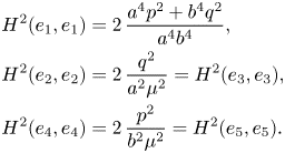
Now, we compute the symmetric $2$ -tensor $H^{2}$
 and we see that its non-zero components are the following
As for the Ricci tensor ${{\rm Ric}}_g$ , we choose a $g$
 -orthonormal basis $(E_1,\,E_2,\,E_3,\,E_4,\,E_5)$
 of $\mathfrak {m}$
 , and we compute its components with respect to the basis $\mathcal {B}$
 using the formula [Reference Besse6, 7.38]. Since $\mathfrak {g}$
 is unimodular, this formula reads

for every $X\in \mathfrak {m}$ . Since

and $[e_i,\,e_j]_{\mathfrak {m}} = [e_i,\,e_j]$ otherwise, we obtain that the only non-zero components of ${{\rm Ric}}_g$
 are the following
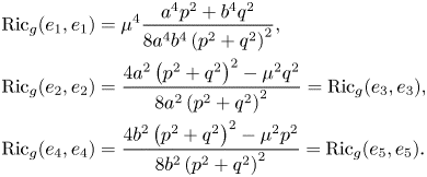
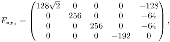
Now, it is easy to see that ${{\rm Ric}}_g = \frac 14 H^{2}$ has a unique solution under the constraints $\mu >0,\,a>0,\,b>0$
 and $p^{2}+q^{2}\neq 0$
 , namely
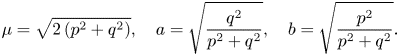
Thus, when $p\neq q$ , the homogeneous space ${{\mathrm M}}_{p,q}={{\mathrm G}}/{{\mathrm K}}_{p,q}$
 admits an invariant metric $g_o$
 and an invariant harmonic form $H_o$
 giving rise to a Bismut Ricci flat connection. Moreover, the pair $(g_o,\,H_o)$
 is unique up to scaling.
Case $\boldsymbol {p= q}$ . We have $p=q=1$
 and the modules $\mathfrak {m}_1$
 and $\mathfrak {m}_2$
 are equivalent. The space of $\textrm{ad} (\mathfrak {k}_{1,1})$
 -invariant 3-forms is given by

with $\dim (\mathfrak {m}_0^{*} \otimes \mathfrak {m}_1^{*}\otimes \mathfrak {m}_2^{*})^{\mathfrak {k}_{1,1}} = 2$ .
.
The generic invariant 3-form $H\in (\Lambda ^{3}\mathfrak {m}^{*})^{\mathfrak {k}_{1,1}}$ has the following expression

where $h_i\in {{\mathbb {R}}}$ , for $i=1,\,2,\,3,\,4$
 . Using the Koszul formula (3.1), we see that $H$
 is closed if and only if $h_2=h_1$
 .
.
The generic invariant metric on $\mathfrak {m}$ is given by
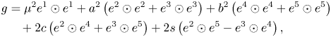
where $\mu,\, a,\, b,\, c,\, s$ are real constants such that

We remark here that it is always possible to assume $s=0$ . Indeed, the one-dimensional torus ${{\mathrm U}}:= \exp (\mathbb {R} e_1)$
 centralizes ${{\mathrm K}}_{1,1}$
 and therefore for every $u\in {{\mathrm U}}$
 we can consider the ${{\mathrm G}}$
 -equivariant diffeomorphism $\tau _u\in {\rm {Dif{}f}}({{\mathrm M}})^{{\mathrm G}}$
 given by $\tau _u(x{{\mathrm K}}_{1,1}) = xu{{\mathrm K}}_{1,1}$
 , for $x\in {{\mathrm G}}$
 . Then, for every $g\in S^{2}(\mathfrak {m})^{\mathfrak {k}_{1,1}}$
 , which is given by the data $(\mu,\,a,\,b,\,c,\,s)$
 as in (3.4), the ${{\mathrm G}}$
 -invariant symmetric tensor $\tau _u^{*}g$
 corresponds to the data $(\mu,\,a,\,b,\,c'=c\,\cos t + s\, \sin t,\,s'= -c\, \sin t + s\, \cos t)$
 , for $u=\exp (te_1)\in {{\mathrm U}}$
 . Therefore, we immediately see that we have $s'=0$
 for an appropriate choice of $u\in {{\mathrm U}}$
 .
.
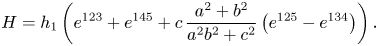
Now, we have
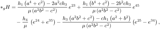
and using again the Koszul formula, we obtain

Thus, $H$ is coclosed if and only if
The generic invariant harmonic 3-form on $\mathfrak {m}$ is then given by
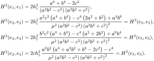
Consequently, the (possibly) non-zero components of the invariant symmetric $2$ -tensor $H^{2}$
 are the following
Let us consider the following $g$ -orthonormal basis of $\mathfrak {m}$

Then, using formula (3.2) and its polarization, and observing that

we obtain the following expressions for the (possibly) non-zero components of the Ricci tensor

We now look for invariant metrics $g$ and harmonic 3-forms $H$
 for which ${{\rm Ric}}_g = \frac 14 H^{2}$
 . A computation using the above expressions of the components of ${{\rm Ric}}_g$
 and $H^{2}$
 shows that we need to find points in the open subset

where all of the following polynomials vanish
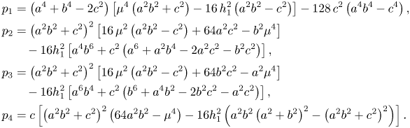
Clearly, the polynomial $p_4$ vanishes if $c=0$
 . When this happens, the remaining polynomials simplify considerably, and they vanish simultaneously if and only if

for some $t>0$ . Therefore, when $c=0$
 , we obtain an invariant BRF pair $(g_o,\,H_o) \in \mathcal {B}({{\mathrm M}}_{1,1})^{{\mathrm G}}$
 that is unique up to scaling and up to a sign in the definition of $H_o$
 , namely

To prove the last assertion, we first consider the set

and we recall that every invariant metric is uniquely determined by the string $(\mu,\,a,\,b,\,c,\,s)$ as in (3.4). We then consider the subset

Every point $(g,\,H)\in \mathcal {P}'$ is uniquely determined by a string $(\mu,\,a,\,b,\,c,\,h_1)\in \mathcal {A} \subset \mathbb {R}^{5}$
 , where $(\mu,\,a,\,b,\,c)$
 determines $g$
 as in (3.4) and $h_1$
 determines $H$
 as in (3.5). The set $\mathcal {B}({{\mathrm M}}_{1,1})^{{{\mathrm G}}} \cap \mathcal {P}'$
 can be identified with the zero set in $\mathcal {A}$
 of the map

Notice that $F(x_o)=0$ , where $x_o=(2\sqrt {2},\,1,\,1,\,0,\,2)\in \mathcal {A}$
 corresponds to the BRF pair $(g_o,\,H_o)$
 , and that $F(\gamma (t))=0\in \mathbb {R}^{4}$
 for every $t\in {{\mathbb {R}}}^{+}$
 , where $\gamma (t) = (2\sqrt {2}t,\,t,\,t,\,0,\,2t^{2})$
 is the curve through $x_o$
 corresponding to $(t^{2}g_o,\,t^{2}H_o)$
 . If we now compute the differential of $F$
 at $x_o$
 , we obtain
and since $\mathrm {rank} (F_{*x_o} ) = 4,$ we see that there exists a neighbourhood $\mathcal {U}'$
 of $(g_o,\,H_o)$
 in $\mathcal {P}'$
 so that $\mathcal {U}' \cap \mathcal {B}({{\mathrm M}}_{1,1})^{{{\mathrm G}}}$
 coincides with the set $\left \{(t^{2}g_o,\,t^{2}H_o) {\ |\ }t\in (1-\varepsilon,\,1+\varepsilon ')\right \}$
 , for suitable $\varepsilon,\,\varepsilon ' >0$
 .
.
We now use the ${{\mathrm G}}$ -equivariant diffeomorphisms $\tau _u$
 , $u\in {{\mathrm U}}$
 , to transform every element of $\mathcal {B}({{\mathrm M}}_{1,1})^{{{\mathrm G}}}\cap \mathcal {P}$
 into an element of $\mathcal {B}({{\mathrm M}}_{1,1})^{{{\mathrm G}}}\cap \mathcal {P}'$
 via $\tau _u^{*}$
 . Note that for every $u\in {{\mathrm U}}$
 we have $(\tau _u^{*}g_o,\,\tau _u^{*}H_o)=(g_o,\,H_o)$
 , since $c=s=0$
 . Moreover, we can easily see that there exists a neighbourhood $\mathcal {U}$
 of $(g_o,\,H_o)$
 in $\mathcal {P}$
 so that $\tau _u^{*}(\mathcal {U})\subseteq \mathcal {U}'$
 . Therefore, if $(g,\,H)\in \mathcal {B}({{\mathrm M}}_{1,1})^{{{\mathrm G}}}\cap \mathcal {U}$
 , then we can find $u\in {{\mathrm U}}$
 so that $\tau _u^{*}(g,\,H)\in \mathcal {B}({{\mathrm M}}_{1,1})^{{{\mathrm G}}}\cap \mathcal {U}'$
 . Hence, $\tau _u^{*}(g,\,H)= (t^{2}g_o,\,t^{2}H_o)$
 , for some $t > 0$
 , and we have $(g,\,H)=\tau _{u^{-1}}^{*}(t^{2}g_o,\,t^{2}H_o) = (t^{2}g_o,\,t^{2}H_o)$
 .
.
Remark 3.4 The Bismut Ricci flat, non-flat manifolds constructed in the previous theorem provide counterexamples to a generalized Alekseevsky–Kimelfeld theorem [Reference Alekseevsky and Kimelfeld4] for the Bismut connection. This question was raised in [Reference Garcia-Fernández and Streets15], cf. Question 3.58. Furthermore, using similar computations, it is not difficult to obtain examples of Bismut connections on ${{\mathrm M}}_{p,q}$ that are Ricci flat and non-flat and whose invariant torsion form $H$
 is not closed. Finally, we also remark here that the Riemannian manifolds $({{\mathrm M}}_{p,q},\,g_o)$
 are not Einstein.
Remark 3.5 In the proof, we have noticed that the BRF pairs $(g,\,H)$ are unique (up to multiples) when $p\neq q$
 . When $p=q=1$
 , we have given the full description of all possible invariant metrics and relative harmonic $3$
 -forms. Unfortunately, the complexity of the computations prevented us from finding other solutions.
Remark 3.6 We remark that the $3$ -form $H$
 we have constructed in the Riemannian spaces $({{\mathrm M}}_{p,q},\,g)$
 is harmonic but never parallel with respect to the Bismut connection. Indeed, if it were, then we would have $dH = 2\sigma _H = 0$
 , where $\sigma _H$
 is the fundamental $4$
 -form $\sigma _H=\frac 12 \sum _{i=1}^{5}\imath _{v_i}H\wedge \imath _{v_i}H$
 and $\{v_i\}$
 is a local orthonormal frame (see e.g. [Reference Friedrich and Ivanov12]). By [Reference Agricola, Ferreira and Friedrich2, Thm. 4.1], we would then have that ${{\mathrm M}}_{p,q}$
 is a compact simple Lie group, a contradiction.
3.1 The Kobayashi's construction
The manifolds ${{\mathrm M}}_{p,q}$ naturally appear as principal $S^{1}$
 -bundles over ${{\mathrm {SU}}}(2)^{2}/{{\mathbb {T}}}^{2}\cong S^{2}\times S^{2}$
 . In this section, we briefly review a useful construction, due to Kobayashi [Reference Kobayashi17], which allows to obtain new geometric structures on principal $S^{1}$
 -bundles over some base manifold $B$
 . This might lead to a generalization of our examples.
Given a compact manifold $B$ , it is well known that there is a one-to-one correspondence between principal $S^{1}$
 -bundles $\pi :P\to B$
 and elements in $H^{2}(B,\,\mathbb {Z})$
 . Given a closed $2$
 -form $\alpha$
 with $[\alpha ]\in {H}^{2}(B,\,\mathbb {Z})$
 , there exists a principal $S^{1}$
 -bundle $\pi :P\to B$
 and a connection form $\gamma$
 so that $d\gamma =\pi ^{*}\alpha$
 . If $B$
 is equipped with a Riemannian metric $g_o$
 , we can construct a Riemannian metric $g$
 on $P$
 by setting $g := c^{2}\gamma \odot \gamma + \pi ^{*}g_o$
 , for some $c>0$
 . Following [Reference Kobayashi17], we compute the Ricci curvature as follows: if $X,\,Y$
 are horizontal tangent vectors and $v$
 is a unit vertical tangent vector, we have

where for every $2$ -form $\omega$
 on $B$
 we define $\hat \omega \in S^{2}(T^{*}B)$
 as $\hat \omega (Z,\,W) = g_o(\imath _Z\omega,\,\imath _W\omega )$
 , for every tangent vector fields $Z,\,W\in \Gamma (TB)$
 , and we let $||\omega ||^{2}= g_o(\hat \omega,\,\hat \omega )$
 .
.
We now prove a result that might be useful to construct new examples of BRF pairs on suitable manifolds. In particular, this result allows to reduce the problem of finding harmonic $3$ -forms on a certain manifold to a problem on the existence of suitable harmonic $2$
 -forms on a lower dimensional manifold.
Proposition 3.7 Given a compact Riemannian manifold $(B,\,g_o)$ and a non-zero harmonic $2$
 -form $\alpha$
 with $[\alpha ]\in {H}^{2}(B,\,\mathbb {Z})$
 , the associated principal $S^{1}$
 -bundle $P$
 over $B$
 admits a BRF pair $(g,\,H)$
 if there exist a harmonic form $\beta \in \Omega ^{2}(B)$
 and positive numbers $\lambda,\,\mu \in \mathbb {R}^{+}$
 so that the following conditions are fulfilled:
(a) $\alpha \wedge \beta =0;$
(b) $||\beta ||^{2} = \lambda ||\alpha ||^{2}$
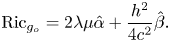
at every point of $B;$(c) the Ricci tensor ${{\rm Ric}}_{g_o}$
satisfies the equation
\[ {{\rm Ric}}_{g_o} = 2 \lambda\mu \hat \alpha + \mu\hat \beta. \]


Proof. We consider the metric $g= c^{2}\gamma \odot \gamma + \pi ^{*}g_o$ with $c^{2}=\lambda \mu$
 . We then define a $3$
 -form $H\in \Omega ^{3}(P)$
 as
as
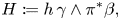
for some $h\in \mathbb {R}$ . Searching for conditions implying that $(g,\,H)$
 is a BRF pair, we see that $H$
 is closed if and only if $\alpha \wedge \beta =0$
 and $\beta$
 is closed, while it is coclosed if and only if $d(\pi ^{*}(*_{g_o}\beta ))=0$
 , i.e., $\beta$
 is coclosed. Therefore, $H$
 is $g$
 -harmonic if and only if $\beta$
 is $g_o$
 -harmonic and condition (a) holds. Looking now at the expression of the Ricci tensor of $g$
 , we see that $\alpha$
 being harmonic implies that ${{\rm Ric}}_g(V,\,Z)$
 vanishes whenever $V$
 is vertical and $Z$
 is horizontal. As we easily check, $H^{2}(Z,\,V)=0$
 as well. Thus, we only need to verify the following


where $X,\,Y$ are vector fields on $B$
 and $v$
 is a unit vertical field on $P$
 . Now, using (b), we have
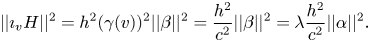
Hence, equation (3.7) reads
whence

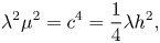
As for equation (3.6), we see that $H^{2}(X,\,Y)=\frac {h^{2}}{c^{2}} \hat \beta (X,\,Y)$ so that (3.6) reads
This coincides with the expression of the Ricci tensor as in (c) when we use $c^{2}=\lambda \mu$ and the expression (3.8) for the constant $h$
 .
.
Remark 3.8 Our examples on the manifolds ${{\mathrm M}}_{p,q}$ can be seen as special cases of the above construction.
4. The asymptotic behaviour of the solution to the GRF on ${{\mathrm M}}_{p,q}$

In this last section, we consider the homogeneous space ${{\mathrm M}}_{p,q} = {{\mathrm G}}/{{\mathrm K}}_{p,q}$ , $p\neq q$
 , with the BRF pair $(g_o,\,H_o)$
 determined in the proof of theorem 3.3, and we study the behaviour of the homogeneous generalized Ricci flow (1.2) on ${{\mathrm M}}_{p.q}$
 . We have the following.
Theorem 4.1 Let $(g_t,\,H_t)$ be the invariant solution to the generalized Ricci flow on ${{\mathrm M}}_{p,q}$
 , $p\neq q$
 , starting at an invariant pair $(g,\,H)$
 with $dH=0$
 at $t=t_o$
 . Then, $H_t = \lambda H_o$
 , for some $\lambda \in \mathbb {R}^{+}$
 , the solution $(g_t,\,H_t)$
 exists for all $t\geq t_o$
 and it converges to the BRF pair $(\lambda g_o,\,\lambda H_o)$
 as $t\rightarrow +\infty$
 .
.
We begin showing that the proof of theorem 4.1 reduces to the qualitative study of a suitable system of ordinary differential equations. Let $(g_t,\,H_t)$ be an invariant solution to the generalized Ricci flow on ${{\mathrm M}}_{p,q}$
 , $p\neq q$
 . It follows from the discussion in the proof of theorem 3.3 that

and

where $\mu _t,\,a_t,\,b_t,\,\lambda _t$ are positive real valued functions of $t$
 .
.
The BRF pair $(g_o,\,H_o)$ is a fixed point of the generalized Ricci flow, thus the solution to the flow starting from it corresponds to the constant functions

Now, since $H_t$ is $g_t$
 -harmonic, from the second equation in (1.2) we obtain
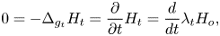
whence it follows that $\lambda _t =\lambda \in {{\mathbb {R}}}^{+}$ is a positive constant and thus $H_t =\lambda H_o$
 . We now consider the first equation in (1.2)
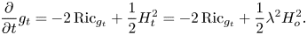
Using again our previous computations, we see that this equation is equivalent to an autonomous system of ODEs for the functions $\mu _t,\,a_t,\,b_t$ . If we let $M_t:= \mu _t^{2}$
 , $A_t:= a_t^{2}$
 , $B_t:= b_t^{2}$
 , then the system is the following:
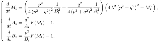
where
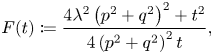
The fixed point of this system is given by $x_{o,\lambda } := (\lambda \mu _o^{2},\, \lambda a_o^{2},\, \lambda b_o^{2})$ and it corresponds to the invariant metric $\lambda g_o$
 .
.
Now, the proof of theorem 4.1 follows from the next result.
Proposition 4.2 The solution $(M_t,\,A_t,\,B_t)$ to the system (4.1) starting at any given triplet of positive numbers $(M_o,\,A_o,\,B_o)$
 at $t=t_o$
 exists for all $t \geq t_o$
 and it converges to the fixed point $x_{o,\lambda }$
 as $t\rightarrow +\infty$
 .
.
Proof. Let
and let $I=[t_o,\,T)$ be the maximal existence interval for the solution $(M_t,\,A_t,\,B_t)$
 . We divide the discussion into various steps. step 1. If $M_t$
 assumes the value $\overline M$
 for some $\overline {t} \in I$
 , then $M_t=\overline M$
 for all $t\in I$
 , $T=+\infty$
 and $\lim _{t\to +\infty }A_t= q^{2}F(\overline M)$
 , $\lim _{t\to +\infty }B_t= p^{2}F(\overline M)$
 . Indeed, let $(\overline A_t,\,\overline B_t)$
 be the solution of the system
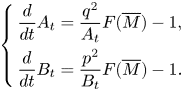
with initial conditions $(\overline A_{t_o}= A_{t_o},\,\overline B_{t_o}= B_{t_o})$ . Then, $(\overline A_t,\,\overline B_t,\, M_t=\overline M)$
 satisfies the system (4.1) and therefore we have $M_t=\overline M$
 for every $t\in I$
 by uniqueness. Now, it is clear that $q^{2}F(\overline M)$
 and $p^{2}F(\overline M)$
 are particular solutions of the first and second equation of (4.2), respectively. Therefore, either $A_t$
 , $B_t$
 are constant, or their derivatives never vanish. This implies that $A_t$
 and $B_t$
 remain bounded from above and from below by two positive constants. Then, $|A_t'|$
 and $|B_t'|$
 are uniformly bounded, and this implies the long time existence and the convergence by standard arguments.
step 2. $M_t$ is monotone and for every $t\in I$
 we have either $M_t\in [M_o,\,\overline M]$
 or $M_t\in [\overline M,\,M_o]$
 . In fact, $M_t'$
 never vanishes unless $M_t$
 is constant. Therefore, $M_t$
 is increasing (resp. decreasing) if $M_o<\overline M$
 (resp. $M_o>\overline M$
 ). In particular, the limit $\lim _{t\to T}M_t$
 exists.
step 3. We have $T=+\infty$ . Suppose $T<+\infty$
 . We consider the first equation in (4.1). First of all, we note that $A_t$
 is bounded on $I$
 . Indeed, by step 2, $C_1 \leq F(M_t) \leq C_2$
 on $I$
 for some positive constants $C_1,\,C_2$
 , hence $A_t' \leq \frac {q^{2}{C_2}}{A_t}$
 , and thus $(A_t^{2})'\leq q^{2}C_2$
 and $A_t\leq \sqrt {q^{2}C_2t+A_o^{2}}\leq C_3:= \sqrt {q^{2}C_2T+A_o^{2}}$
 for all $t\in I$
 . In turn this implies that $A_t'\geq \frac {q^{2}{C_1}}{C_3}-1$
 , so that $|A_t'|$
 is uniformly bounded. Consequently, the limit $\lim _{t\to T}A_t$
 exists, call it $\alpha \geq 0$
 . We need to prove that $\alpha \neq 0$
 . Let us put $y_t=A_t^{2}$
 , so that $y' = -2\sqrt {y} + 2q^{2}F(M_t)$
 . If $\alpha =0$
 , then $\lim _{t\to T}y'(t) = \lim _{t\to T}q^{2}F(M_t) >0$
 . This is impossible as it implies that $y(t)<0$
 in a suitable left neighbourhood of $T$
 . The same argument applies to $B_t$
 and our claim follows.
step 4. If there exists a constant $K>0$ so that $A_t'\leq -1 + \frac {K}{A_t}$
 , then for every $\epsilon >0$
 there exists some $T_\epsilon$
 such that
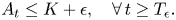
The same statement holds for $B_t$ . As a consequence, the functions $A_t$
 and $B_t$
 are bounded on $[t_o,\,+\infty )$
 . If we put $y(t)=A_t^{2}$
 as before, then we have $y'\leq -2\sqrt {y} + 2\,K$
 . First, we note that the inequality $A_t> K+\epsilon$
 cannot hold on a half-line $[\tilde {t},\,+\infty )$
 . Indeed, in that case we would have $y'(t)\leq -2\epsilon$
 , hence for some constant $C$
 we would obtain $y(t)\leq -2\epsilon t+C<0$
 for sufficiently large $t$
 , a contradiction. Thus, there exists a point $\overline {t}$
 where $A_{\overline {t}} \leq K+\epsilon$
 . We claim that $A_t\leq K+\epsilon$
 for every $t\geq \overline {t}$
 . Indeed, suppose there exists $t_1> \overline {t}$
 with $A_{t_1}>K+\epsilon$
 and consider $t_2\in [\overline {t},\,t_1]$
 so that $A_{t_2} = \max _{[\overline {t},\,t_1]}A_t$
 . If $t_2\in (\overline {t},\,t_1)$
 , then $0 = A_{t_2}'\leq -1 + \frac {K}{A_{t_2}}$
 , so that $A_{t_2}\leq K$
 , a contradiction. Otherwise, $t_2=t_1$
 and therefore $A_{t_1}'\geq 0$
 implying again $A_{t_1}\leq K$
 . This proves our first claim. By step 2, $M_t$
 takes values into an interval $[C_1,\,C_2]$
 with $C_1>0$
 and therefore $F(M_t)$
 is bounded above by a constant $K$
 . By the previous arguments, $A_t$
 (and similarly $B_t$
 ) is bounded on some positive half-line, hence on $[t_o,\,+\infty )$
 .
.
step 5. We have $\lim _{t\to +\infty } M_t = \overline M$ . Indeed, $M_t$
 is monotone and bounded by step 2, hence the limit $\lim _{t\to +\infty } M_t =m$
 exists. Suppose that $m \neq \overline M$
 . By step 4, the functions $A_t,\,B_t$
 are bounded, hence by the first equation in (4.1) there is a constant $C$
 so that for sufficiently large $t$
contradicting the boundedness of $M_t$ .
.
step 6. We have $\lim _{t\to +\infty }A_t = q^{2} F(\overline M)$ and $\lim _{t\to +\infty }B_t = p^{2} F(\overline M)$
 . We know that $\lim _{t\to +\infty } M_t = \overline M$
 , hence $q^{2}F(M_t) \to q^{2}F(\overline M) =: \phi >0$
 . This means that for every $\epsilon >0$
 there exists $S_\epsilon >0$
 so that $\phi -\epsilon \leq q^{2}F(M_t)\leq \phi +\epsilon$
 for all $t\geq S_\epsilon$
 . By step 4, there exists $T_\epsilon$
 so that for every $t\geq T_\epsilon$
 we have $A_t\leq \phi +2\epsilon$
 . Using similar arguments as in the proof of step 4, we have another point (say again $T_\epsilon$
 ), so that $A_t\geq \phi -2\epsilon$
 for all $t\geq T_\epsilon$
 . Our claim for $A_t$
 is then proved, and the same arguments apply for $B_t$
 .
.
Remark 4.3 The analogous study of the behaviour of the generalized Ricci flow on ${{\mathrm M}}_{1,1}$ is much more involved, due to the presence of off-diagonal terms in the invariant symmetric tensors.
Acknowledgements
The authors were supported by GNSAGA of INdAM and by the project PRIN 2017 ‘Real and Complex Manifolds: Topology, Geometry and Holomorphic Dynamics’. The authors warmly thank Jeffrey Streets and Mario Garcia-Fernández for useful and constructive comments on a preliminary version of this work.


 Open access