1. Introduction
As galaxies evolve over time, signatures of their evolution remain in both the spatial distribution and kinematics of their ionised gas (Stevens, Croton, & Mutch Reference Stevens, Croton and Mutch2016; Osman & Bekki Reference Osman and Bekki2017; Lagos et al. Reference Lagos2018; Bryant et al. Reference Bryant2019; Jiménez et al. Reference Jiménez, Lagos, Ludlow and Wisnioski2022). By studying these disturbances (or lack thereof) in the line-of-sight velocity distribution (LOSVD) of the emitting ionised gas, we can understand the physical mechanisms that contribute to galaxy evolution. Galaxies, however, rarely evolve in isolation and a longstanding goal of galaxy evolution studies is to understand the balance between internal and external galaxy formation processes that contribute to their evolution (i.e., nature vs nurture; Henriksen Reference Henriksen2009)
The observed star-formation rates (SFRs) and cold gas masses in massive galaxies at
 $z=1-3$
suggest that galaxies should exhaust their supply of gas within a few Gyr (Tacconi et al. Reference Tacconi2013), but a number of galaxies within the local universe (
$z=1-3$
suggest that galaxies should exhaust their supply of gas within a few Gyr (Tacconi et al. Reference Tacconi2013), but a number of galaxies within the local universe (
 $z \sim 0$
) are still readily forming stars (Bigiel et al. Reference Bigiel2008, Reference Bigiel2010); this suggests that galaxies have a means of replenishing their cold gas supply to continue forming stars. This can be accomplished through several internal and external mechanisms. An example of an internal mechanism would be a star-forming galaxy’s gravitational potential being deep enough to hold on to, and re-accrete the gas after it is expelled from either supernovae (SNe) or stellar winds; causing a galactic ‘fountain’ effect (Shapiro & Field Reference Shapiro and Field1976; Spitoni, Recchi, & Matteucci Reference Spitoni, Recchi and Matteucci2008; Marinacci et al. Reference Marinacci2010). Conversely, rather than ‘recycling’ expelled gas, galaxies can externally accrete fresh gas from the hot outer halo (
$z \sim 0$
) are still readily forming stars (Bigiel et al. Reference Bigiel2008, Reference Bigiel2010); this suggests that galaxies have a means of replenishing their cold gas supply to continue forming stars. This can be accomplished through several internal and external mechanisms. An example of an internal mechanism would be a star-forming galaxy’s gravitational potential being deep enough to hold on to, and re-accrete the gas after it is expelled from either supernovae (SNe) or stellar winds; causing a galactic ‘fountain’ effect (Shapiro & Field Reference Shapiro and Field1976; Spitoni, Recchi, & Matteucci Reference Spitoni, Recchi and Matteucci2008; Marinacci et al. Reference Marinacci2010). Conversely, rather than ‘recycling’ expelled gas, galaxies can externally accrete fresh gas from the hot outer halo (
 $T \sim 10^6$
K), along cold (
$T \sim 10^6$
K), along cold (
 $T \sim 10^4$
K) cosmological filaments or through interactions and mergers with other galaxies (Kereš et al. Reference Davà Kereš, Katz, Weinberg and Davé2005; Dekel et al. Reference Dekel2009; Di Teodoro & Fraternali Reference Di Teodoro and Fraternali2014; Pezzulli, Fraternali, & Binney Reference Pezzulli, Fraternali and Binney2017; Wright et al. Reference Wright and Lagos2021; Kamphuis et al. Reference Kamphuis2022). For both the ‘cold’ or ‘hot’ modes, theory predicts that external gas accretion is a source of stellar-gas kinematic misalignments (i.e., difference between the rotation position angle (PA
$T \sim 10^4$
K) cosmological filaments or through interactions and mergers with other galaxies (Kereš et al. Reference Davà Kereš, Katz, Weinberg and Davé2005; Dekel et al. Reference Dekel2009; Di Teodoro & Fraternali Reference Di Teodoro and Fraternali2014; Pezzulli, Fraternali, & Binney Reference Pezzulli, Fraternali and Binney2017; Wright et al. Reference Wright and Lagos2021; Kamphuis et al. Reference Kamphuis2022). For both the ‘cold’ or ‘hot’ modes, theory predicts that external gas accretion is a source of stellar-gas kinematic misalignments (i.e., difference between the rotation position angle (PA
 $_{kin}$
) of the stars and gas; Bryant et al. Reference Bryant2019), although the internal properties of the galaxy affect whether the gas can realign or not (Lagos et al. Reference Lagos2015; Casanueva et al. Reference Casanueva and Lagos2022).
$_{kin}$
) of the stars and gas; Bryant et al. Reference Bryant2019), although the internal properties of the galaxy affect whether the gas can realign or not (Lagos et al. Reference Lagos2015; Casanueva et al. Reference Casanueva and Lagos2022).
Gas is rarely stationary within the galactic disk, rotating with bulk motion as well as moving with a series of inflows and outflows. These gaseous flows onto the central regions of galaxies can trigger a galaxy’s Active Galactic Nucleus (AGN), which can contribute to ‘quenching’ the SFR in high stellar mass galaxies (e.g., Schawinski et al. Reference Schawinski2007). AGNs are also a known source of outflows, and can disturb the kinematics of the entire galactic disk (e.g., Greene et al. Reference Greene, Zakamska, Ho and Barth2011; Zakamska et al. Reference Zakamska2016) and are a suspected cause of complex kinematic features in a velocity maps (Juneau et al. Reference Juneau2022).
The surrounding environment can have complex effects on a galaxy’s SFR; ram-pressure stripping (RPS) caused by the hot intra-cluster medium and galaxy-galaxy interactions can readily quench the SFR in satellite galaxies through cold gas stripping (see Cortese, Catinella, & Smith Reference Cortese, Catinella and Smith2021, for a review), but can enhance the SFR in the most massive galaxy of a major merging pair (Davies et al. Reference Davies2015). In either case, these interactions can cause the kinematics to deviate significantly from disk-like rotation (Taylor, Federrath, & Kobayashi Reference Taylor, Federrath and Kobayashi2018; McElroy et al. Reference McElroy2022).
Galaxy kinematics are extremely sensitive to both external and internal galaxy formation processes. By quantifying kinematic disturbances in galaxy velocity maps, we can better understand which physical processes dominate in their evolution. Integral Field Spectroscopic (IFS) instruments can collect spatially resolved spectra and can construct 2-dimensional kinematic maps of the stars and ionised gas phase in galaxies. In the last decade, IFS surveys (e.g., SINS; Förster Schreiber et al. Reference Förster Schreiber2006, ATLAS
 $^{\rm 3D}$
; Cappellari et al. Reference Cappellari2011, SAMI; Bryant et al. Reference Bryant2015, MaNGA; Bundy et al. Reference Bundy2015, CALIFA; Sánchez et al. Reference Sánchez2016) have revealed the wide range of complex kinematic features and the disturbed kinematics that galaxies can display. These disturbances have been linked to external processes such as gas stripping and mergers (e.g., Bellhouse et al. Reference Bellhouse2017; Bloom et al. Reference Bloom2018; Feng et al. Reference Feng, Shen, Yuan, Riffel and Pan2020; Ristea et al. Reference Ristea2022), and internal processes such as star-formation, torques provided from a bar or the presence of an AGN (e.g., Barrera-Ballesteros et al. Reference Barrera-Ballesteros2014; Holmes et al. Reference Holmes2015; Bloom et al. Reference Bloom2017a; Florian et al. Reference Florian2020).
$^{\rm 3D}$
; Cappellari et al. Reference Cappellari2011, SAMI; Bryant et al. Reference Bryant2015, MaNGA; Bundy et al. Reference Bundy2015, CALIFA; Sánchez et al. Reference Sánchez2016) have revealed the wide range of complex kinematic features and the disturbed kinematics that galaxies can display. These disturbances have been linked to external processes such as gas stripping and mergers (e.g., Bellhouse et al. Reference Bellhouse2017; Bloom et al. Reference Bloom2018; Feng et al. Reference Feng, Shen, Yuan, Riffel and Pan2020; Ristea et al. Reference Ristea2022), and internal processes such as star-formation, torques provided from a bar or the presence of an AGN (e.g., Barrera-Ballesteros et al. Reference Barrera-Ballesteros2014; Holmes et al. Reference Holmes2015; Bloom et al. Reference Bloom2017a; Florian et al. Reference Florian2020).
The dynamics of stars and gas in galaxies are largely driven by the gravitational potential, and hence the mass distribution of the dark matter and baryons (i.e., the stars and gas, see Binney & Tremaine Reference Binney and Tremaine2008; Brough et al. Reference Brough2017; Rutherford et al. Reference Rutherford2021), however van de Sande et al. (Reference van de Sande2021) show that galactic environment is also a significant driver. It is expected that external mechanisms such as galaxy-galaxy interactions or environmental effects (i.e., ram-pressure and viscous stripping) will produce a more significant kinematic disturbance in the outskirts where the gravitational potential is shallower than near the centre. This can be tested by comparing kinematic disturbances at inner and outer radial extents. A study using local, gas-rich galaxies in the HI-SAMI survey (Catinella et al. Reference Catinella2023) compared the asymmetry measured in global atomic Hydrogen (HI) and H
 $\alpha$
velocity profiles (Watts et al. Reference Watts2023a). The authors report that the global HI asymmetry is driven mostly by external mechanisms (mergers and interactions), but did not find a straight-forward connection between the asymmetries of the two gas phases.
$\alpha$
velocity profiles (Watts et al. Reference Watts2023a). The authors report that the global HI asymmetry is driven mostly by external mechanisms (mergers and interactions), but did not find a straight-forward connection between the asymmetries of the two gas phases.
In this work, we further explore the sources of kinematic asymmetry by measuring the asymmetry confined to the optical disk by using a single gas phase (the ionised gas), rather than two different gas phases as was done in Watts et al. (Reference Watts2023a). We measure the asymmetry at the
 $0.5Re$
(inner) and at
$0.5Re$
(inner) and at
 $1.5Re$
(outer) elliptical annuli, and investigate whether kinematic asymmetries vary with galactocentric radius. We use data from the Middle Ages Galaxy Properties in Integral field spectroscopy Survey (MAGPI, Foster et al. Reference Foster2021), a Very Large Telescope/Multi-Unit Spectroscopic Explorer (VLT-MUSE) Large Program, to investigate whether the kinematics of galaxies do become more perturbed at larger radii. We use kinemetry (Krajnović et al. Reference Krajnović2006) to quantify kinematic asymmetries as is commonly used in IFS surveys (Shapiro et al. Reference Shapiro2008; Krajnović et al. Reference Krajnović2011; Bloom et al. Reference Bloom2017a; Feng et al. Reference Feng, Shen, Yuan, Riffel and Pan2020). The structure of this paper is as follows: Section 2 gives a brief overview of the MAGPI survey, our data and sample selection. In Section 3 we describe the three kinemetry models used in this work. In Section 4 we discuss our results, the strength of each model and possible implications for galaxy evolution before offering some concluding remarks in Section 5.
$1.5Re$
(outer) elliptical annuli, and investigate whether kinematic asymmetries vary with galactocentric radius. We use data from the Middle Ages Galaxy Properties in Integral field spectroscopy Survey (MAGPI, Foster et al. Reference Foster2021), a Very Large Telescope/Multi-Unit Spectroscopic Explorer (VLT-MUSE) Large Program, to investigate whether the kinematics of galaxies do become more perturbed at larger radii. We use kinemetry (Krajnović et al. Reference Krajnović2006) to quantify kinematic asymmetries as is commonly used in IFS surveys (Shapiro et al. Reference Shapiro2008; Krajnović et al. Reference Krajnović2011; Bloom et al. Reference Bloom2017a; Feng et al. Reference Feng, Shen, Yuan, Riffel and Pan2020). The structure of this paper is as follows: Section 2 gives a brief overview of the MAGPI survey, our data and sample selection. In Section 3 we describe the three kinemetry models used in this work. In Section 4 we discuss our results, the strength of each model and possible implications for galaxy evolution before offering some concluding remarks in Section 5.
We adopt a Planck Collaboration et al. (2020) cosmology for this work; explicitly a flat Universe with
 $H_0$
= 67.7 kms
$H_0$
= 67.7 kms
 $^{-1}$
Mpc
$^{-1}$
Mpc
 $^{-1}$
,
$^{-1}$
,
 $\Omega_{\rm M}$
= 0.31 and
$\Omega_{\rm M}$
= 0.31 and
 $\Omega_\Lambda$
= 0.69.
$\Omega_\Lambda$
= 0.69.
2. Data
In this section, we briefly describe the MAGPI survey and the data products we use, followed by a description of our selection process and the subsample.
2.1 The MAGPI survey
The MAGPI survey is an ongoing Large Program on the VLT/MUSE targeting 56
 $\sim$
1
$\sim$
1
 $\times$
1 arcmin fields (currently 41 completed). MAGPI data are spatially resolved spectra of stars and ionised gas focusing on the redshift range z = 0.28–0.35 selected from three of the Galaxy and Mass Assembly (GAMA, Driver et al. Reference Driver2011) fields: G12, G15 and G23. MAGPI also includes archival MUSE observations from the legacy fields Abell 370 and Abell 2477. When observations are completed, the main MAGPI sample will comprise spatially resolved spectroscopy for 60 ‘primary’ targets (M
$\times$
1 arcmin fields (currently 41 completed). MAGPI data are spatially resolved spectra of stars and ionised gas focusing on the redshift range z = 0.28–0.35 selected from three of the Galaxy and Mass Assembly (GAMA, Driver et al. Reference Driver2011) fields: G12, G15 and G23. MAGPI also includes archival MUSE observations from the legacy fields Abell 370 and Abell 2477. When observations are completed, the main MAGPI sample will comprise spatially resolved spectroscopy for 60 ‘primary’ targets (M
 $_*$
$_*$
 $\geq$
7
$\geq$
7
 $\times$
10
$\times$
10
 $^{10}$
M
$^{10}$
M
 $_\odot$
) and
$_\odot$
) and
 $\sim$
100 spatially resolved satellites (M
$\sim$
100 spatially resolved satellites (M
 $_*$
$_*$
 $\geq$
10
$\geq$
10
 $^9$
M
$^9$
M
 $_\odot$
). A detailed description of the survey and its aims are discussed in Foster et al. (Reference Foster2021).
$_\odot$
). A detailed description of the survey and its aims are discussed in Foster et al. (Reference Foster2021).
Data are taken with the MUSE Wide Field Mode in the nominal wavelength range (4 650–9 300 Å) with a spectral sampling of 1.25 Å. Ground-layer adaptive optics is used to mitigate the effects of atmospheric seeing, resulting in a 270 Å-wide gap between 5 780 Å and 6 050 Å due to the GALACSI laser notch filter. Each MAGPI field has a field-of-view of 1x1 square arcminutes with spatial sampling of 0.2′′ pixel
 $^{-1}$
and the average image quality of 0.65′′ FWHM. A detailed discussion of the data reduction will be presented in the first data release (Mendel et al. in preparation).
$^{-1}$
and the average image quality of 0.65′′ FWHM. A detailed discussion of the data reduction will be presented in the first data release (Mendel et al. in preparation).
There are a number of high-level data products currently available to the MAGPI team. Stellar masses for this paper are derived via broadband photometry SED fitting, using 9-band u-Ks imaging data collated for the GAMA survey. To derive the photometric measurements for MAGPI sources, these images were first pixel-matched to the MAGPI cubes (ensuring that the pixel scales were identical), and then the MAGPI segmentation maps presented by Foster et al. (Reference Foster2021) were used to extract forced photometry per object. These photometry were then used for SED fitting with the code ProSpect (Robotham et al. Reference Robotham2020) to provide a range of galaxy properties. These stellar masses are extracted in the standard approach as done in the most recent GAMA analysis (Bellstedt et al. Reference Bellstedt2020; Driver et al. Reference Driver2022), and in Derkenne et al. (Reference Derkenne2023). A truncated skewed-Normal parametrisation is used for the star-formation history, with a linearly evolving metallicity evolution implemented to ensure a chemical build-up that follows the stellar mass build-up in the galaxy. A Chabrier (Reference Chabrier2003) Initial Mass Function (IMF) is assumed, and the Bruzual & Charlot (Reference Bruzual and Charlot2003) stellar population templates are used.
We also use Sérsic indices computed from 2-dimensional surface brightness fitting using galfit (Peng et al. Reference Peng, Ho, Impey and Rix2002, Reference Peng, Ho, Impey and Rix2010). We model the two-dimensional surface brightness distribution in mock i-band images computed from the MAGPI cubes. We adopt a model of the reconstructed point spread function (PSF) derived using muse-psfr (Fusco et al. Reference Fusco2020) as described by Mendel et al. (in preparation). In addition to the primary galaxy being fitted (i.e., the galaxy of interest), we include in our fit neighbouring galaxies within
 $\Delta m_i = 5$
mag and projected separations
$\Delta m_i = 5$
mag and projected separations
 $R_p < 5(R_\mathrm{e,primary} + R_\mathrm{e,neighbour})$
. All other sources in the image are masked according to the segmentation image generated by ProFound (Robotham et al. Reference Robotham2018). Before fitting we estimate and remove the local sky background around each source using neighbouring sky pixels (i.e., pixels outside of the dilated ProFound segment mask in the i-band image). Our choice of using MAGPI mock i-band images for deriving Sérsic indexes is motivated by the MAGPI data themselves providing the most uniform coverage in terms of depth, image quality and availability of ancillary data.
$R_p < 5(R_\mathrm{e,primary} + R_\mathrm{e,neighbour})$
. All other sources in the image are masked according to the segmentation image generated by ProFound (Robotham et al. Reference Robotham2018). Before fitting we estimate and remove the local sky background around each source using neighbouring sky pixels (i.e., pixels outside of the dilated ProFound segment mask in the i-band image). Our choice of using MAGPI mock i-band images for deriving Sérsic indexes is motivated by the MAGPI data themselves providing the most uniform coverage in terms of depth, image quality and availability of ancillary data.
We also use emission line products, in particular continuum subtracted fluxes and kinematic maps, that are described in Battisti et al. (in preparation), Briefly, the emission line products were derived using GIST (Galaxy IFU Spectroscopy Tool; Bittner et al. Reference Bittner2019), a python wrapper of pPXF (Cappellari & Emsellem Reference Cappellari and Emsellem2004; Cappellari Reference Cappellari2017) and GandALF (Sarzi et al. Reference Sarzi2006; Falcón-Barroso et al. Reference Falcón-Barroso2006). Gas velocity and dispersion maps are derived from single component Gaussian fits to spectral lines in the continuum subtracted spectra ranging from [OII]3 727Å to [SII]6 733Å; velocity and dispersion measurements for all lines are then tied to brightest line (H
 $\alpha$
for our redshift range). We use H
$\alpha$
for our redshift range). We use H
 $\alpha$
fluxes measured from the Gaussian fit to calculate a SFR within 1.5
$\alpha$
fluxes measured from the Gaussian fit to calculate a SFR within 1.5
 $R_e$
for each of the galaxies in our sample. We correct for dust attenuation assuming an intrinsic Balmer decrement of H
$R_e$
for each of the galaxies in our sample. We correct for dust attenuation assuming an intrinsic Balmer decrement of H
 $\alpha$
/H
$\alpha$
/H
 $\beta$
= 2.86 and the extinction curve from Cardelli, Clayton, & Mathis (Reference Cardelli, Clayton and Mathis1989) with a reddening factor
$\beta$
= 2.86 and the extinction curve from Cardelli, Clayton, & Mathis (Reference Cardelli, Clayton and Mathis1989) with a reddening factor
 $R_V$
=3.1. We use the H
$R_V$
=3.1. We use the H
 $\alpha$
SFR calibration from Calzetti (Reference Calzetti, Falcón-Barroso and Knapen2013), which implicitly assumes a Kroupa (Reference Kroupa2001) IMF. Following Bernardi et al. (Reference Bernardi2010), we multiply our SFR calibration by 1.22 to correct for the Kroupa (Reference Kroupa2001) IMF and continue with a Chabrier (Reference Chabrier2003) IMF for our subsequent analysis.
$\alpha$
SFR calibration from Calzetti (Reference Calzetti, Falcón-Barroso and Knapen2013), which implicitly assumes a Kroupa (Reference Kroupa2001) IMF. Following Bernardi et al. (Reference Bernardi2010), we multiply our SFR calibration by 1.22 to correct for the Kroupa (Reference Kroupa2001) IMF and continue with a Chabrier (Reference Chabrier2003) IMF for our subsequent analysis.
For environment metrics for MAGPI galaxies, we use results from the group-finding algorithm, ‘Parliment’Footnote a (Harborne et al. in preparation). In particular, the comoving distance to the nearest neighbour
 $d_1$
in the groups that Parliment found in each of the MAGPI fields. Parliment follows the methodology in Knobel et al. (Reference Knobel2009). Briefly, galaxies were determined to be within a group if the angular and line-of-sight separation were less than the perpendicular and parallel linking lengths, respectively. The parallel and perpendicular linking lengths for galaxy i were calculated as:
$d_1$
in the groups that Parliment found in each of the MAGPI fields. Parliment follows the methodology in Knobel et al. (Reference Knobel2009). Briefly, galaxies were determined to be within a group if the angular and line-of-sight separation were less than the perpendicular and parallel linking lengths, respectively. The parallel and perpendicular linking lengths for galaxy i were calculated as:
 \begin{equation} l_{\perp,i} = \textit{min}\left(L_{\textit{max}}\times(1+z_i),\frac{b}{\bar{n}^{(1/3)}}\right) \end{equation}
and
 \begin{equation} l_{\parallel,i} = R\ l_{\perp,i} \end{equation}
where
 $\bar{n}=0.01$
Mpc
$\bar{n}=0.01$
Mpc
 $^{-3}$
was the assumed number density of galaxies (Fossati et al. Reference Fossati2019) and
$^{-3}$
was the assumed number density of galaxies (Fossati et al. Reference Fossati2019) and
 $L_{\max}$
, b and R are the free parameters of the algorithm.
$L_{\max}$
, b and R are the free parameters of the algorithm.
2.2 Sample selection
We select those galaxies from the GAMA fields G12, G15 and G23 such that they are within MAGPI’s primary redshift range (0.28
 $<z_{\rm spec}<$
0.35) and have an effective radius
$<z_{\rm spec}<$
0.35) and have an effective radius
 $R_e$
(i.e., radius containing half the i-band light from the galaxy) larger than 0.7′′, which is 0.05′′ larger than the estimated PSF in each MAGPI field. Our redshift and size cutoff ensures we only target galaxies at this predicted ‘epoch of transformation’ and are sufficiently resolved. Finally, we remove those galaxies where the maximum H
$R_e$
(i.e., radius containing half the i-band light from the galaxy) larger than 0.7′′, which is 0.05′′ larger than the estimated PSF in each MAGPI field. Our redshift and size cutoff ensures we only target galaxies at this predicted ‘epoch of transformation’ and are sufficiently resolved. Finally, we remove those galaxies where the maximum H
 $\alpha$
flux SNR
$\alpha$
flux SNR
 $<$
20. This reduces the entire MAGPI catalogue to 61 galaxies. If a galaxy satisfies these criteria, we mask any spaxels on the velocity map were the H
$<$
20. This reduces the entire MAGPI catalogue to 61 galaxies. If a galaxy satisfies these criteria, we mask any spaxels on the velocity map were the H
 $\alpha$
flux SNR
$\alpha$
flux SNR
 $<$
3.
$<$
3.
For our parent sample of 61 galaxies, most galaxies in our sample sit along the Star Forming Main Sequence (SFMS; Daddi et al. Reference Daddi2007; Speagle et al. Reference Speagle, Steinhardt, Capak and Silverman2014; Thorne et al. Reference Thorne2021) with 39 galaxies within
 $\pm$
0.3 dex of the SFMS (see bottom right panel of Fig. 1) defined for MAGPI galaxies at
$\pm$
0.3 dex of the SFMS (see bottom right panel of Fig. 1) defined for MAGPI galaxies at
 $z\sim0.35$
(Mun et al. in preparation). It is not surprising that our sample mostly consists of star-forming galaxies, since one selection criterion we invoked was a sufficient detection of H
$z\sim0.35$
(Mun et al. in preparation). It is not surprising that our sample mostly consists of star-forming galaxies, since one selection criterion we invoked was a sufficient detection of H
 $\alpha$
in emission. Looking at Sérsic indices only for galaxies where the fit has converged (i.e.,
$\alpha$
in emission. Looking at Sérsic indices only for galaxies where the fit has converged (i.e.,
 $\chi^2$
<10), these 29 galaxies (48% of the parent sample) consists mostly of ‘disky’ galaxies with the mean and median 2D Sérsic indices n being 1.27 and 0.9, respectively (e.g., bottom left panel Fig. 1). The sample consists of mostly massive galaxies (
$\chi^2$
<10), these 29 galaxies (48% of the parent sample) consists mostly of ‘disky’ galaxies with the mean and median 2D Sérsic indices n being 1.27 and 0.9, respectively (e.g., bottom left panel Fig. 1). The sample consists of mostly massive galaxies (
 $\log$
(M
$\log$
(M
 $_*$
/M
$_*$
/M
 $_\odot$
)>10) with a mean and median of 10.17 and 10.18, respectively (e.g., top left panel Fig. 1). Looking at the environments the galaxies in our sample inhabit, they inhabit low to high-density environments. The median and mean group multiplicity of our sample is 6 and 7, respectively (e.g., top right panel of Fig. 1).
$_\odot$
)>10) with a mean and median of 10.17 and 10.18, respectively (e.g., top left panel Fig. 1). Looking at the environments the galaxies in our sample inhabit, they inhabit low to high-density environments. The median and mean group multiplicity of our sample is 6 and 7, respectively (e.g., top right panel of Fig. 1).
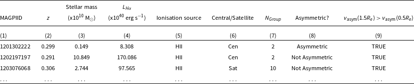
Table 1. Col. 1: MAGPIID, Col. 2: spectroscopic redshift, Col. 3: Stellar Mass, Col. 4: Integrated H
 $\alpha$
luminosity within
$\alpha$
luminosity within
 $1.5R_e$
, Col. 5: Source of ionisation in the galaxy, Col 6.: Is the galaxy the Central or a satellite to the group? A dash indicates no data was available, Col 7.: Number of galaxies within the group containing the galaxy, a dash indicates that no data was available, Col 8.: Is the galaxy asymmetric globally? (i.e.,
$1.5R_e$
, Col. 5: Source of ionisation in the galaxy, Col 6.: Is the galaxy the Central or a satellite to the group? A dash indicates no data was available, Col 7.: Number of galaxies within the group containing the galaxy, a dash indicates that no data was available, Col 8.: Is the galaxy asymmetric globally? (i.e.,
 $\langle v_{\rm aysm} \rangle>0.04$
), Col 9.: Does the galaxy have higher asymmetric outskirts? (i.e.,
$\langle v_{\rm aysm} \rangle>0.04$
), Col 9.: Does the galaxy have higher asymmetric outskirts? (i.e.,
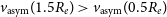 $v_{\rm asym} (1.5R_e) > v_{\rm asym}(0.5R_e)$
). Dashes indicate where data was not available. The remaining rows of the table are provided as supplementary material.
$v_{\rm asym} (1.5R_e) > v_{\rm asym}(0.5R_e)$
). Dashes indicate where data was not available. The remaining rows of the table are provided as supplementary material.


Figure 1. Histograms of galactic properties for the parent MAGPI sample and the subsample used in this study. The parent MAGPI sample is shown in grey, whereas our subsample is shown in blue. Mean values for each property in the subsample are shown as magenta vertical lines in each panel. Median values for each property in the parent sample are shown as dark blue lines. Top Left: Histogram of the stellar masses for the MAGPI galaxies and our sample. Top Right: Histogram of the number of galaxies within the group containing the galaxy. Bottom Left: Histogram of the Sérsic indices. Only galaxies with a
 $\chi^2$
<10 from the surface-brightness fitting are shown in blue. Bottom Right: Star formation rate vs. stellar mass. Cyan lines represents the error bars in stellar mass and star formation rate. The magenta line shown is the fitted Main Sequence for the MAGPI galaxies at
$\chi^2$
<10 from the surface-brightness fitting are shown in blue. Bottom Right: Star formation rate vs. stellar mass. Cyan lines represents the error bars in stellar mass and star formation rate. The magenta line shown is the fitted Main Sequence for the MAGPI galaxies at
 $z=0.35$
.
$z=0.35$
.
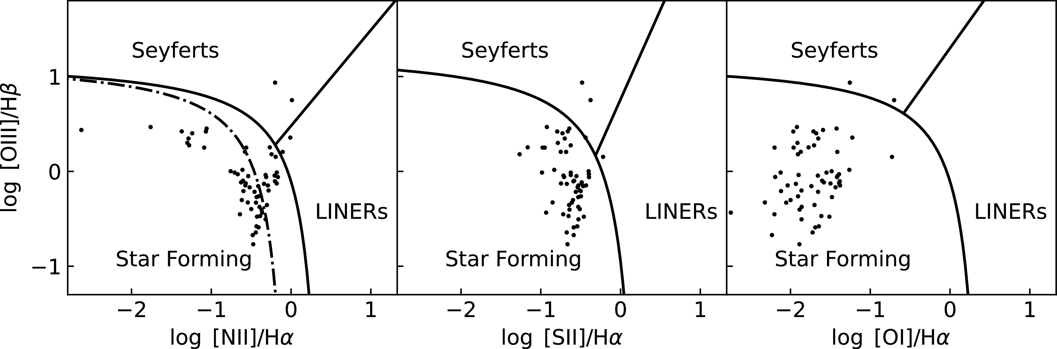
Figure 2. A [NII]-BPT (left), [SII]-BPT (middle), and [OI]-BPT (right) diagram of our sample. The hyperbolic solid lines in all three panels are from criterion suggested in Kauffmann et al. (Reference Kauffmann2003). The dashed line in the left panel is the cut-off for HII regions, while the solid line is the cut-off for AGNs. The straight line in the [NII]-BPT is the separation of Seyfert and LINERs suggested in Cid Fernandes et al. (Reference Cid Fernandes2010). The straight lines in [SII]-BPT and [OI]-BPT separate Seyfert, LINER and HII as per Kewley et al. (Reference Kewley, Groves, Kauffmann and Heckman2006).
Finally, we used BPT diagnostic plots (Baldwin, Phillips, & Terlevich Reference Baldwin, Phillips and Terlevich1981) and the criteria stipulated in Kauffmann et al. (Reference Kauffmann2003) and Kewley et al. (Reference Kewley, Groves, Kauffmann and Heckman2006), shown in Fig. 2, to classify which galaxies in our sample are star-forming, host an AGN, or have HII+AGN ionisation. To be consistent with our calculated SFRs, we use integrated fluxes within 1.5
 $R_e$
, masking spaxels where the SNR
$R_e$
, masking spaxels where the SNR
 $<$
3 for each line. For a galaxy to be classified as a Seyfert or a Low Ionisation Nuclear Region (LINER), we require consistent classification across the three [NII]-BPT, [SII]-BPT and [OI]-BPT plots, and it not be in the HII+AGN section of the [NII]-BPT. Our sample consists of star-forming galaxies (43/61; 70%), galaxies with HII+AGN ionisation (16/61; 26%) and a small number of Seyferts (2/54; 3%). No LINERs were detected consistently across all three BPT diagrams, but one is detected using the [SII]-BPT diagram. A table of physical properties is shown in Table 1.
$<$
3 for each line. For a galaxy to be classified as a Seyfert or a Low Ionisation Nuclear Region (LINER), we require consistent classification across the three [NII]-BPT, [SII]-BPT and [OI]-BPT plots, and it not be in the HII+AGN section of the [NII]-BPT. Our sample consists of star-forming galaxies (43/61; 70%), galaxies with HII+AGN ionisation (16/61; 26%) and a small number of Seyferts (2/54; 3%). No LINERs were detected consistently across all three BPT diagrams, but one is detected using the [SII]-BPT diagram. A table of physical properties is shown in Table 1.
3. Kinemetric analysis
kinemetry (Krajnović et al. Reference Krajnović2006) is a generalisation of photometric techniques for higher order moments of the LOSVD (e.g., mean velocity, disperision, h
3, h
4; Gerhard Reference Gerhard1993; van der Marel & Franx Reference van der Marel and Franx1993). These kinematic moments can be symmetric, with either even parity (point-symmetric) or odd parity (point-antisymmetric); kinemetry fits a model to the LOSVD moment maps using a series of concentric ellipses with position angle (PA) and axial ratio q, where
 $q=b/a$
and b and a are the semi-minor and semi-major axes, respectively. Similar to other tilted ring fitting algorithms (Rogstad, Lockhart, & Wright Reference Rogstad, Lockhart and Wright1974; Franx, van Gorkom, & de Zeeuw Reference Franx, van Gorkom and de Zeeuw1994; Spekkens & Sellwood Reference Spekkens and Sellwood2007), kinemetry fits a Fourier Series along the ellipse as follows:
$q=b/a$
and b and a are the semi-minor and semi-major axes, respectively. Similar to other tilted ring fitting algorithms (Rogstad, Lockhart, & Wright Reference Rogstad, Lockhart and Wright1974; Franx, van Gorkom, & de Zeeuw Reference Franx, van Gorkom and de Zeeuw1994; Spekkens & Sellwood Reference Spekkens and Sellwood2007), kinemetry fits a Fourier Series along the ellipse as follows:
 \begin{equation} K(a,\theta) = A_0 + \sum_{N=1}^{N=n} [A_n\sin{(n\theta)} + B_n\cos{(n\theta)}], \end{equation}
where a is the semi-major axis of the ellipse,
 $\theta$
is the azimuth along the ellipse with respect to the semi-major axis, A
$\theta$
is the azimuth along the ellipse with respect to the semi-major axis, A
 $_0$
is the zeroth harmonic term and A
$_0$
is the zeroth harmonic term and A
 $_n$
and B
$_n$
and B
 $_n$
are the
$_n$
are the
 $n\rm{th}$
additional harmonic terms. kinemetry determines the best fitting ellipses by minimising the harmonic coefficients that are in the series. Equation (3) can be equivalently represented as:
$n\rm{th}$
additional harmonic terms. kinemetry determines the best fitting ellipses by minimising the harmonic coefficients that are in the series. Equation (3) can be equivalently represented as:
 \begin{equation} K(a,\theta) = A_0 + \sum_{n=1}^{n=N} k_n\cos{(n[\theta - \phi_n(a)])}, \end{equation}
where
 $k_n = \sqrt{A_n^2+B_n^2}$
and
$k_n = \sqrt{A_n^2+B_n^2}$
and
 $\phi = \arctan\frac{A_n}{B_n}$
. One can extract the
$\phi = \arctan\frac{A_n}{B_n}$
. One can extract the
 $k_n$
values, which describes the kinematics of the galaxy, and the PA and q parameters, which describe the geometry of the ellipse. If a galaxy is rotating with perfect circular motion, it can be completely described using Equation (3) with a single cosine term, which would be symmetrical in the azimuthal axis at 180
$k_n$
values, which describes the kinematics of the galaxy, and the PA and q parameters, which describe the geometry of the ellipse. If a galaxy is rotating with perfect circular motion, it can be completely described using Equation (3) with a single cosine term, which would be symmetrical in the azimuthal axis at 180
 $^{\circ}$
. Any deviations from circular motion would result in asymmetric function, and these asymmetries would be encoded as power (i.e., a non-zero values in the A
$^{\circ}$
. Any deviations from circular motion would result in asymmetric function, and these asymmetries would be encoded as power (i.e., a non-zero values in the A
 $_n$
and B
$_n$
and B
 $_n$
terms where
$_n$
terms where
 $n>1$
) in the higher-order coefficients in Equation (3) (see Fig. A.2 for an example of what these asymmetries look like). The first moment of the LOSVD (the recessional velocity map) is an odd moment, and it was suggested by Krajnović et al. (Reference Krajnović2006) that only odd harmonic terms (
$n>1$
) in the higher-order coefficients in Equation (3) (see Fig. A.2 for an example of what these asymmetries look like). The first moment of the LOSVD (the recessional velocity map) is an odd moment, and it was suggested by Krajnović et al. (Reference Krajnović2006) that only odd harmonic terms (
 $k_1,k_3,k_5$
) in Equation (4) are needed to sufficiently describe ellipses along this moment. The subsequent moment following the recessional velocity map (the dispersion map) is an even moment of the LOSVD; and rather than only odd harmonic terms, both even and odd harmonic terms are needed. For the purposes of this work, we only focus on the first moment of the LOSVD, i.e. the recessional velocity map.
$k_1,k_3,k_5$
) in Equation (4) are needed to sufficiently describe ellipses along this moment. The subsequent moment following the recessional velocity map (the dispersion map) is an even moment of the LOSVD; and rather than only odd harmonic terms, both even and odd harmonic terms are needed. For the purposes of this work, we only focus on the first moment of the LOSVD, i.e. the recessional velocity map.
kinemetry has been previously used on a number of IFS surveys to quantify the asymmetry in the stellar velocity and dispersion maps. The ATLAS
 $^{3D}$
survey (Cappellari et al. Reference Cappellari2011) used kinemetry to describe their sample as either ‘regular’ or ‘non-regular’ rotators (RR, NRR) by whether the luminosity-weighted average
$^{3D}$
survey (Cappellari et al. Reference Cappellari2011) used kinemetry to describe their sample as either ‘regular’ or ‘non-regular’ rotators (RR, NRR) by whether the luminosity-weighted average
 $\langle{k_5/k_1}\rangle$
reached above 0.04 (Krajnović et al. Reference Krajnović2011). A similar criterion was adopted for the SAMI Galaxy Survey (Bryant et al. Reference Bryant2015; Bloom et al. Reference Bloom2017a,b), where those with
$\langle{k_5/k_1}\rangle$
reached above 0.04 (Krajnović et al. Reference Krajnović2011). A similar criterion was adopted for the SAMI Galaxy Survey (Bryant et al. Reference Bryant2015; Bloom et al. Reference Bloom2017a,b), where those with
 $\langle{k_5/k_1}\rangle < 0.04$
were described as RR, those with
$\langle{k_5/k_1}\rangle < 0.04$
were described as RR, those with
 $\langle{k_5/k_1}\rangle$
between 0.04 and 0.08 as quasiregular rotators and those with
$\langle{k_5/k_1}\rangle$
between 0.04 and 0.08 as quasiregular rotators and those with
 $\langle{k_5/k_1}\rangle > 0.08$
as NRRs (van de Sande et al. Reference van de Sande2021). For this paper, we adopt a definition of a galaxy being ‘asymmetric’ if
$\langle{k_5/k_1}\rangle > 0.08$
as NRRs (van de Sande et al. Reference van de Sande2021). For this paper, we adopt a definition of a galaxy being ‘asymmetric’ if
 $v_{\rm asym}>0.04$
(Krajnović et al. Reference Krajnović2011).
$v_{\rm asym}>0.04$
(Krajnović et al. Reference Krajnović2011).
kinemetry is agnostic to the source of the emission and can be used on velocity maps of both the stars and gas in galaxies. The Spectroscopic Imaging survey in the Near-infrared with SINFONI (SINS; Förster Schreiber et al. Reference Förster Schreiber2006) survey defined the asymmetry in the H
 $\alpha$
velocity field as,
$\alpha$
velocity field as,
 \begin{equation} v_{\rm asym,SINS} =\frac{k_2+k_3+k_4+k_5}{4k_1}, \end{equation}
where
 $v_{\rm asym}$
is averaged over the entire disk. The units of
$v_{\rm asym}$
is averaged over the entire disk. The units of
 $k_n$
will be dependent on the map being modelled; in our case for a velocity map, the units are in kms
$k_n$
will be dependent on the map being modelled; in our case for a velocity map, the units are in kms
 $^{-1}$
, hence
$^{-1}$
, hence
 $v_{\rm asym}$
is a dimensionless quantity. They included the even terms as major mergers are expected to cause large kinematic disturbances, and so even terms would be needed to adequately model the data. They found that
$v_{\rm asym}$
is a dimensionless quantity. They included the even terms as major mergers are expected to cause large kinematic disturbances, and so even terms would be needed to adequately model the data. They found that
 $v_{\rm asym,SINS}$
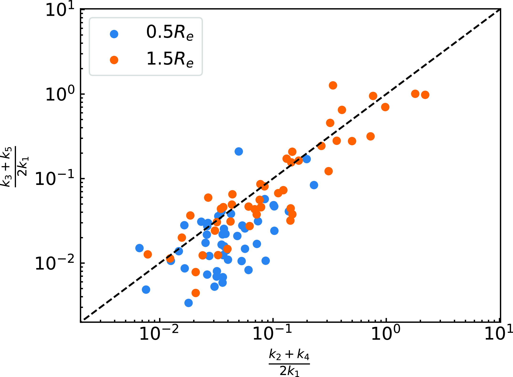
was a reliable proxy to distinguish disk and merging systems (Shapiro et al. Reference Shapiro2008). In contrast, Bloom et al. (Reference Bloom2017a,b) choose to only include the odd terms and compute the mean of the ratio of the higher order to first order moments over all radii (
$v_{\rm asym,SINS}$
was a reliable proxy to distinguish disk and merging systems (Shapiro et al. Reference Shapiro2008). In contrast, Bloom et al. (Reference Bloom2017a,b) choose to only include the odd terms and compute the mean of the ratio of the higher order to first order moments over all radii (
 $v_{\rm asym}$
) as follows:
$v_{\rm asym}$
) as follows:
 \begin{equation} v_{\rm asym,SAMI} = \frac{k_3+k_5}{2k_1}. \end{equation}
Their choice of only including odd terms was due to negligible power being distributed to the even terms for their sample. They found that kinematically asymmetric galaxies scattered below the Tully-Fisher Relation (TFR; Tully & Fisher Reference Tully and Fisher1977) and that kinematic asymmetry in the gas is inversely correlated with stellar mass (Kannappan, Fabricant, & Franx Reference Kannappan, Fabricant and Franx2002; Cortese et al. Reference Cortese2014; Bloom et al. Reference Bloom2017b).

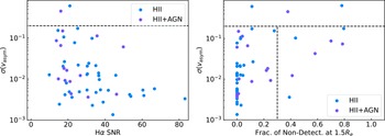
Figure 3.
Left: Uncertainty in
 $v_{asym}$
against the average SNR at that ellipse. HII+AGN galaxies have a magenta edges. When calculating the SNR, we run kinemetry on the SNR map and fix the ellipses to same PA and q values that are returned when running kinemetry on the velocity map. The dashed black line is our adoptive cutoff in uncertainty to remove galaxies from our sample. Right: Uncertainty in
$v_{asym}$
against the average SNR at that ellipse. HII+AGN galaxies have a magenta edges. When calculating the SNR, we run kinemetry on the SNR map and fix the ellipses to same PA and q values that are returned when running kinemetry on the velocity map. The dashed black line is our adoptive cutoff in uncertainty to remove galaxies from our sample. Right: Uncertainty in
 $v_{asym}$
against the fraction of non-detected spaxels at the 1.5
$v_{asym}$
against the fraction of non-detected spaxels at the 1.5
 $R_e$
ellipse. As well as excluding galaxies where the uncertainty is larger than 0.2, we also remove galaxies with more than 30% missing data along the ellipse.
$R_e$
ellipse. As well as excluding galaxies where the uncertainty is larger than 0.2, we also remove galaxies with more than 30% missing data along the ellipse.

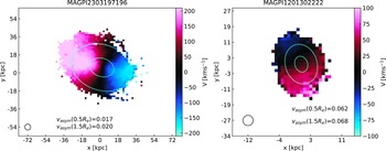
Figure 4. Gas velocity maps of a symmetric (left) and asymmetric (right) galaxy, where an asymmetric galaxy is defined as
 $\langle v_{\rm asym} \rangle>0.04$
. MAGPI2303197196 is a rather normal rotating galaxy, whereas MAGPI120130222 is a slower-rotating galaxy with a complicated velocity structure. The cyan ellipses correspond to
$\langle v_{\rm asym} \rangle>0.04$
. MAGPI2303197196 is a rather normal rotating galaxy, whereas MAGPI120130222 is a slower-rotating galaxy with a complicated velocity structure. The cyan ellipses correspond to
 $0.5R_e$
and
$0.5R_e$
and
 $1.5R_e$
, respectively. The estimated PSF for each galaxy is shown as a circle in the lower left corner.
$1.5R_e$
, respectively. The estimated PSF for each galaxy is shown as a circle in the lower left corner.
For this study, we focus on measuring the kinematic asymmetry present in a sample of MAGPI galaxies at
 $0.5R_e$
and
$0.5R_e$
and
 $1.5R_e$
to study how the kinematic disturbances change with galactocentric distance. We tested three different kinemetry models:
$1.5R_e$
to study how the kinematic disturbances change with galactocentric distance. We tested three different kinemetry models:
-
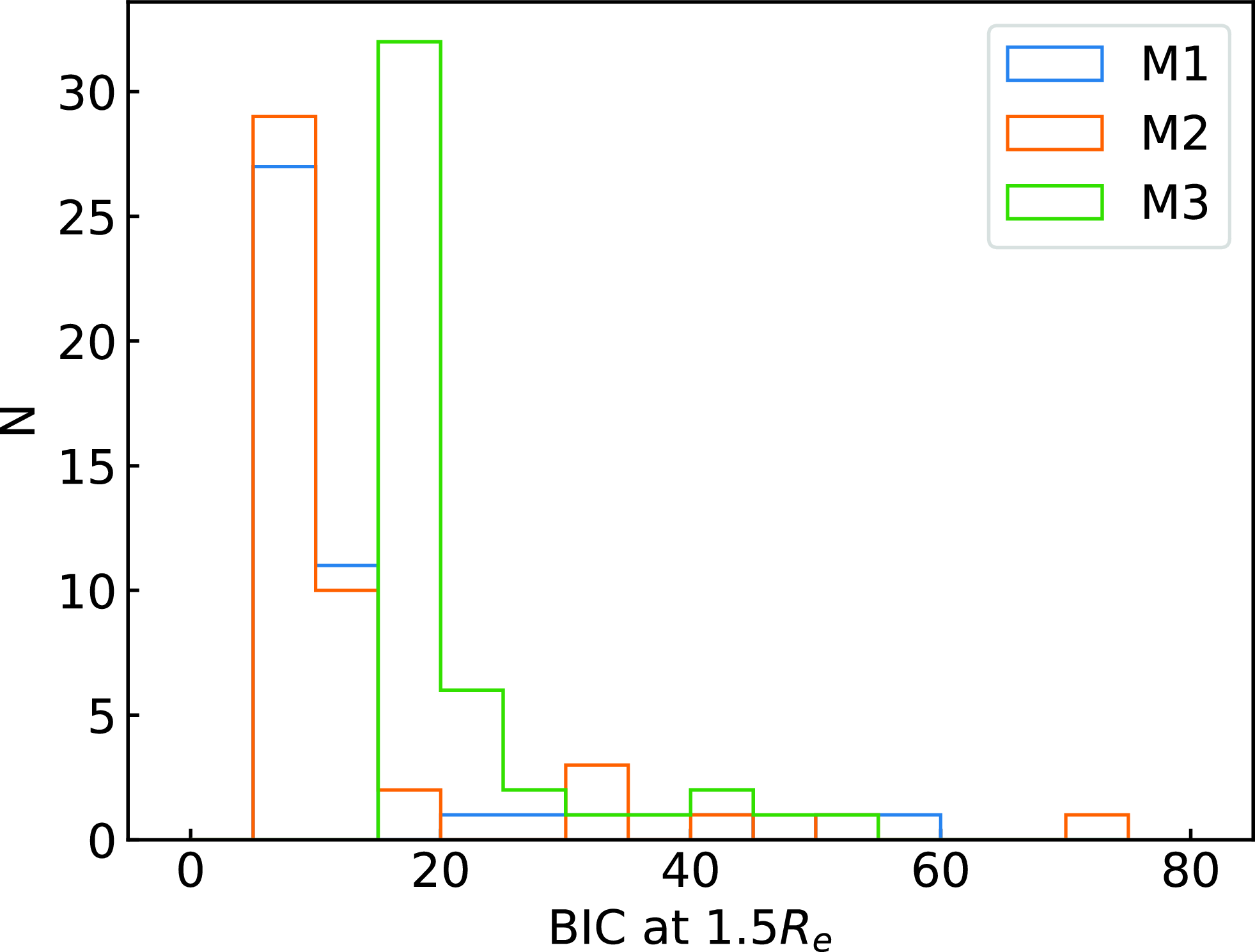
• M1: the first model includes only odd terms (i.e.,
 $k_1,k_3,k_5$
) and the centre fixed on the brightest pixel;
$k_1,k_3,k_5$
) and the centre fixed on the brightest pixel; -
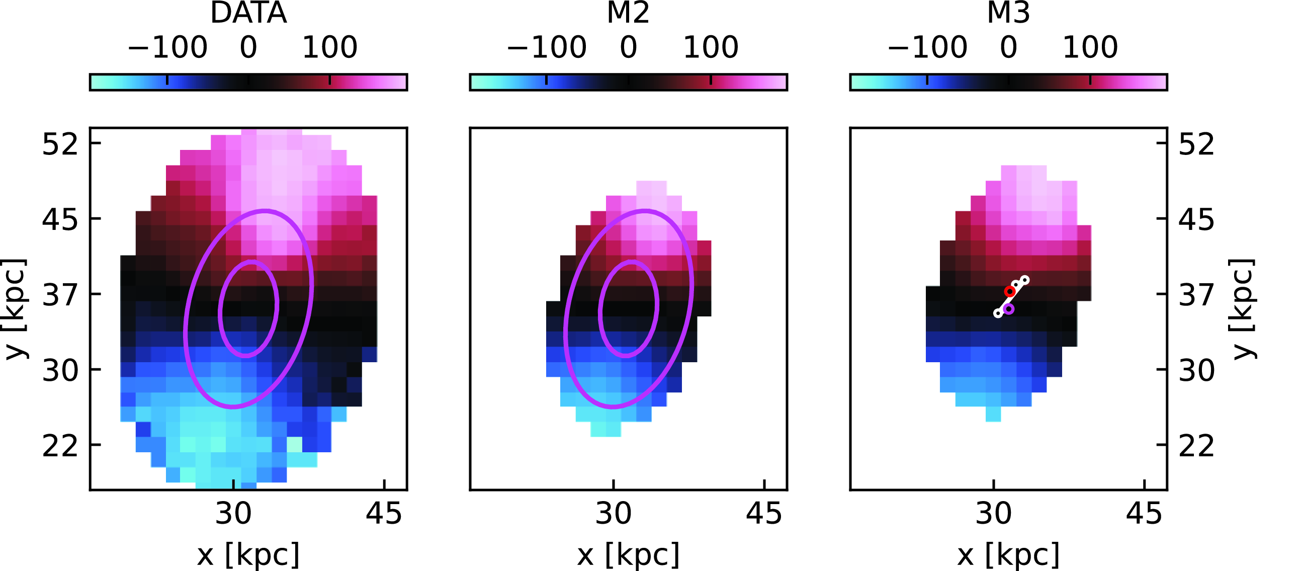
• M2: the second model includes odd and even terms (i.e.,
$k_1,k_2,k_3,k_4,k_5$
) and the centre fixed on the brightest pixel; and finally, -
• M3: the third model includes only odd terms (i.e.,
$k_1,k_3,k_5$
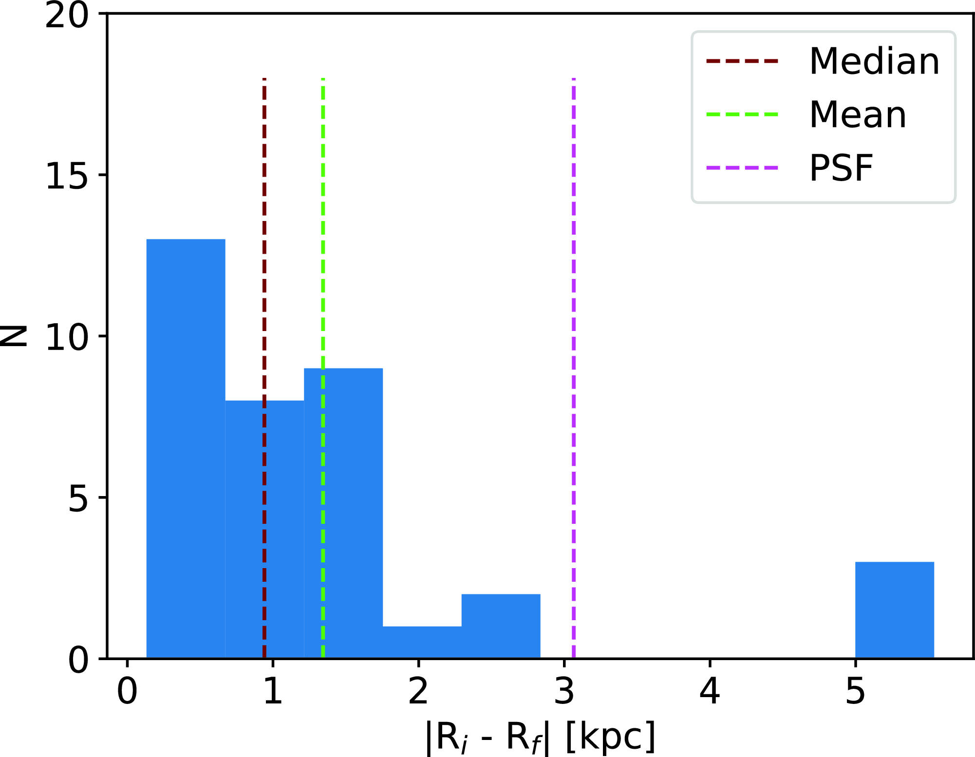
), but the position of the centre is allowed to vary.


For models M1 and M3, we define the asymmetry following Equation (6), and for model M2, we define the asymmetry following Equation (5). We use the
 $v_{\rm asym}$
values fitted at
$v_{\rm asym}$
values fitted at
 $0.5R_e$
and
$0.5R_e$
and
 $1.5R_e$
applying equal weighting to each spaxel along the ellipse. Across all three models, we initially set the kinematic PA and axis ratio to coincide with their photometric counterparts (i.e.
$1.5R_e$
applying equal weighting to each spaxel along the ellipse. Across all three models, we initially set the kinematic PA and axis ratio to coincide with their photometric counterparts (i.e.
 $PA_{\rm kin}=PA_{\rm phot}$
). The initial kinematic centre is assumed to be located at the coordinates of the brightest pixel in the MUSE i-band. We set parameter boundaries as follows:
$PA_{\rm kin}=PA_{\rm phot}$
). The initial kinematic centre is assumed to be located at the coordinates of the brightest pixel in the MUSE i-band. We set parameter boundaries as follows:
 $PA_{kin}$
=[0,360] degrees and
$PA_{kin}$
=[0,360] degrees and
 $q_{\rm kin}$
=[
$q_{\rm kin}$
=[
 $q_{\rm phot}$
−0.1,
$q_{\rm phot}$
−0.1,
 $q_{\rm phot}$
+0.1]. In addition, and for M3 only, we allow the position of the kinematic centre to vary freely as determined by kinemetry. We use kinemetry with a set of ellipses between
$q_{\rm phot}$
+0.1]. In addition, and for M3 only, we allow the position of the kinematic centre to vary freely as determined by kinemetry. We use kinemetry with a set of ellipses between
 $0.5R_e$
and
$0.5R_e$
and
 $1.5R_e$
with the distance in-between each ellipse equal to half the estimated seeing (
$1.5R_e$
with the distance in-between each ellipse equal to half the estimated seeing (
 $\sim0.3''$
). Uncertainties on
$\sim0.3''$
). Uncertainties on
 $v_{\rm asym}$
are estimated using 100 Monte Carlo realisations, where we re-run kinemetry on the velocity map with Gaussian noise (corresponding to the uncertainty in the velocity measurement) injected to each pixel. The final
$v_{\rm asym}$
are estimated using 100 Monte Carlo realisations, where we re-run kinemetry on the velocity map with Gaussian noise (corresponding to the uncertainty in the velocity measurement) injected to each pixel. The final
 $v_{\rm asym}$
values and uncertainties correspond to the mean and standard deviation of the Monte Carlo distribution. We also calculate a flux-weighted
$v_{\rm asym}$
values and uncertainties correspond to the mean and standard deviation of the Monte Carlo distribution. We also calculate a flux-weighted
 $\langle v_{\rm asym} \rangle$
averaged over 1.5
$\langle v_{\rm asym} \rangle$
averaged over 1.5
 $R_e$
. While we mask spaxels on the velocity maps where H
$R_e$
. While we mask spaxels on the velocity maps where H
 $\alpha$
SNR<3, this leads to discontinuities in the maps that prevent kinemetry from computing asymmetries, we therefore estimate velocity value of these spaxels by taking the median of the adjacent 8 spaxels. See Appendix A for details.
$\alpha$
SNR<3, this leads to discontinuities in the maps that prevent kinemetry from computing asymmetries, we therefore estimate velocity value of these spaxels by taking the median of the adjacent 8 spaxels. See Appendix A for details.
Before conducting any analysis, we remove three galaxies where we are unable to measure the asymmetry at
 $1.5R_e$
, we also remove ten galaxies where the uncertainty in the asymmetry at
$1.5R_e$
, we also remove ten galaxies where the uncertainty in the asymmetry at
 $1.5R_e$
is larger than 0.2 and where we have replaced more than 30% of the spaxels along the
$1.5R_e$
is larger than 0.2 and where we have replaced more than 30% of the spaxels along the
 $1.5R_e$
ellipse (see Fig. 3). These choices in cutoff are necessarily ad-hoc, but we found that this limit prevents us from removing low asymmetry galaxies with small uncertainty and removes galaxies with uncertain values that are due to poor fits from kinemetry, GIST or the fraction of missing data is to high. Galaxies with small
$1.5R_e$
ellipse (see Fig. 3). These choices in cutoff are necessarily ad-hoc, but we found that this limit prevents us from removing low asymmetry galaxies with small uncertainty and removes galaxies with uncertain values that are due to poor fits from kinemetry, GIST or the fraction of missing data is to high. Galaxies with small
 $R_e$
and low SNR are naturally excluded as there are too few spaxels along the ellipse for kinemetry to perform the fitting. Five of the ten galaxies thus removed are HII+AGN galaxies with compact size and low H
$R_e$
and low SNR are naturally excluded as there are too few spaxels along the ellipse for kinemetry to perform the fitting. Five of the ten galaxies thus removed are HII+AGN galaxies with compact size and low H
 $\alpha$
SNR. A further Seyfert galaxy is also removed. We include the other AGN and HII+AGN galaxies where the kinematics are modelled adequately according to the uncertainties in their asymmetry following that expected for purely star-forming galaxies.
$\alpha$
SNR. A further Seyfert galaxy is also removed. We include the other AGN and HII+AGN galaxies where the kinematics are modelled adequately according to the uncertainties in their asymmetry following that expected for purely star-forming galaxies.
One galaxy (MAGPI1207197197) had been excluded from any kinemetric analysis due to a poor fit from GIST, but it is mentioned briefly in Section 4.1 due to it being in the same group as two galaxies in our sample. Examples of typical symmetric and asymmetric galaxies are shown in Fig. 4. The final sample consists of 47 galaxies.
4. Results and discussion
In this section, we investigate the connection between asymmetry and galactic properties of each of the galaxies in our sample. In particular, their environment probed through projected distance to nearest neighbour, whether they host an AGN, and their star-formation activity and stellar mass.
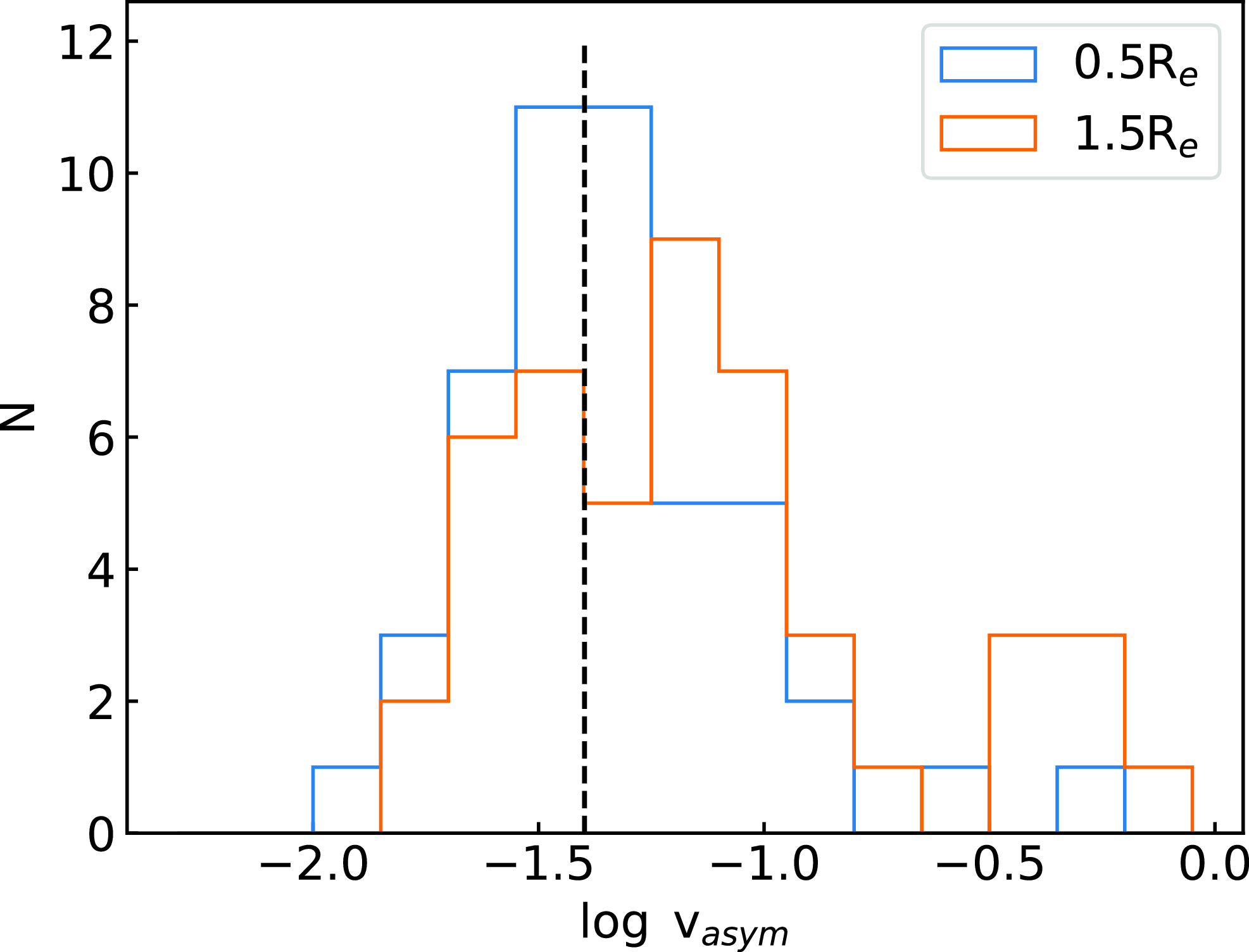
We conduct our analysis using asymmetries calculated with M2. We discuss, in detail, our motivation behind this choice in Appendix A. Using M2, 81
 $^{+6}_{-4}$
%Footnote b of our sample displays larger asymmetry in their outskirts compared to their inner regions, and 46
$^{+6}_{-4}$
%Footnote b of our sample displays larger asymmetry in their outskirts compared to their inner regions, and 46
 $^{+6}_{-7}$
% are asymmetrical at all radii, and a Kolmogorov-Smirnov (KS) test suggests that the distributions of
$^{+6}_{-7}$
% are asymmetrical at all radii, and a Kolmogorov-Smirnov (KS) test suggests that the distributions of
 $v_{asym}(1.5R_e)$
and
$v_{asym}(1.5R_e)$
and
 $v_{asym}(0.5R_e)$
values are different distributions (
$v_{asym}(0.5R_e)$
values are different distributions (
 $t=0.34,p<0.009$
). Fig. 5 shows a histogram of
$t=0.34,p<0.009$
). Fig. 5 shows a histogram of
 $v_{asym}(0.5R_e)$
and
$v_{asym}(0.5R_e)$
and
 $v_{asym}(1.5R_e)$
. Both of these results support the hypothesis that a galaxy’s outer kinematics are more likely to be disturbed. We now discuss possible physical drivers of this.
$v_{asym}(1.5R_e)$
. Both of these results support the hypothesis that a galaxy’s outer kinematics are more likely to be disturbed. We now discuss possible physical drivers of this.
4.1 Environment
The asymmetry in velocity fields is usually attributed to external processes like mergers and interactions (Shapiro et al. Reference Shapiro2008; Bloom et al. Reference Bloom2018; Feng et al. Reference Feng, Shen, Yuan, Riffel and Pan2020) or from ram-pressure stripping from the ICM (Kronberger et al. Reference Kronberger, Kapferer, Unterguggenberger, Schindler and Ziegler2008; Kutdemir et al. Reference Kutdemir2010). For our current subsample, we only have environmental measurements for 42 galaxies. The environmental metrics for MAGPI galaxies are currently incomplete due to limited field of view from MUSE (1′′x1′′), compared to the large GAMA fields they are targeting. Of the 42 galaxies, 15 galaxies are centrals (i.e., the brightest galaxy in the group) with the remaining 27 being satellites. Six central galaxies (5/15; 33%
 $^{+9\%}_{-13\%}$
) are considered globally asymmetric, whereas 20 satellites are globally asymmetric (16/27; 59%
$^{+9\%}_{-13\%}$
) are considered globally asymmetric, whereas 20 satellites are globally asymmetric (16/27; 59%
 $^{+9\%}_{-8\%}$
).
$^{+9\%}_{-8\%}$
).

Figure 5. Histograms of
 $\log v_{asym}$
at
$\log v_{asym}$
at
 $0.5R_e$
(blue) and
$0.5R_e$
(blue) and
 $1.5R_e$
(orange). The black dashed represents our asymmetry cutoff (
$1.5R_e$
(orange). The black dashed represents our asymmetry cutoff (
 $\log v_{asym} =-1.39$
). Both histograms peak at the same values (
$\log v_{asym} =-1.39$
). Both histograms peak at the same values (
 $\log v_{asym}\sim -1.35$
), though the asymmetry values at
$\log v_{asym}\sim -1.35$
), though the asymmetry values at
 $1.5R_e$
are skewed to higher values. A KS-test suggest that we can be confident at the 99.9% level (
$1.5R_e$
are skewed to higher values. A KS-test suggest that we can be confident at the 99.9% level (
 $t=0.34,p<0.009$
) that the each values are drawn from different distributions. The large fraction of galaxies with more asymmetric outskirts and the KS-test results supports our hypothesis that galaxy kinematics are more disturbed at larger galactocentric radius.
$t=0.34,p<0.009$
) that the each values are drawn from different distributions. The large fraction of galaxies with more asymmetric outskirts and the KS-test results supports our hypothesis that galaxy kinematics are more disturbed at larger galactocentric radius.
As two galaxies begin to interact with each other, the outer regions would be more disturbed compared to the inner regions. Interestingly, the fraction of satellite galaxies that are more asymmetric in their outskirts is much larger than centrals with more asymmetric outskirts (93%
 $^{+3\%}_{-2\%}$
vs 66%
$^{+3\%}_{-2\%}$
vs 66%
 $^{+13\%}_{-6\%}$
). This suggests that satellites are much more susceptible to disturbed outskirts than central galaxies.
$^{+13\%}_{-6\%}$
). This suggests that satellites are much more susceptible to disturbed outskirts than central galaxies.
Although interactions between centrals and satellites offers a neat explanation for those groups with both asymmetric centrals and satellites, it does not explain the why the fraction of asymmetric centrals is small while the fraction of asymmetric satellites is large. McElroy et al. (Reference McElroy2022) found that for interacting galaxies with a 2:5 stellar mass ratio in the Feedback In Realistic Environments Simulations (FIRE; Hopkins et al. Reference Hopkins2014, Reference Hopkins2018),
 $v_{\rm asym}$
in the more massive galaxy will peak during the first pass of the interaction but will return to values that are similar to that of an isolated disk galaxy, before peaking again and remaining at high values after coalescence. It could be that the asymmetric satellites in our sample have not made, or have just made, their first passage, hence the central galaxy appears to be symmetric. Rather than being driven by a global group property such as group multiplicity or halo mass, our findings suggest that kinematic asymmetries are likely driven by smaller scale properties, such as projected distance to neighbouring galaxies. This was found to be the case in Feng et al. (Reference Feng, Shen, Yuan, Riffel and Pan2020), who found that the fraction of galaxies with high asymmetry increases when the projected distance between galaxies in close pairs decreases.
$v_{\rm asym}$
in the more massive galaxy will peak during the first pass of the interaction but will return to values that are similar to that of an isolated disk galaxy, before peaking again and remaining at high values after coalescence. It could be that the asymmetric satellites in our sample have not made, or have just made, their first passage, hence the central galaxy appears to be symmetric. Rather than being driven by a global group property such as group multiplicity or halo mass, our findings suggest that kinematic asymmetries are likely driven by smaller scale properties, such as projected distance to neighbouring galaxies. This was found to be the case in Feng et al. (Reference Feng, Shen, Yuan, Riffel and Pan2020), who found that the fraction of galaxies with high asymmetry increases when the projected distance between galaxies in close pairs decreases.

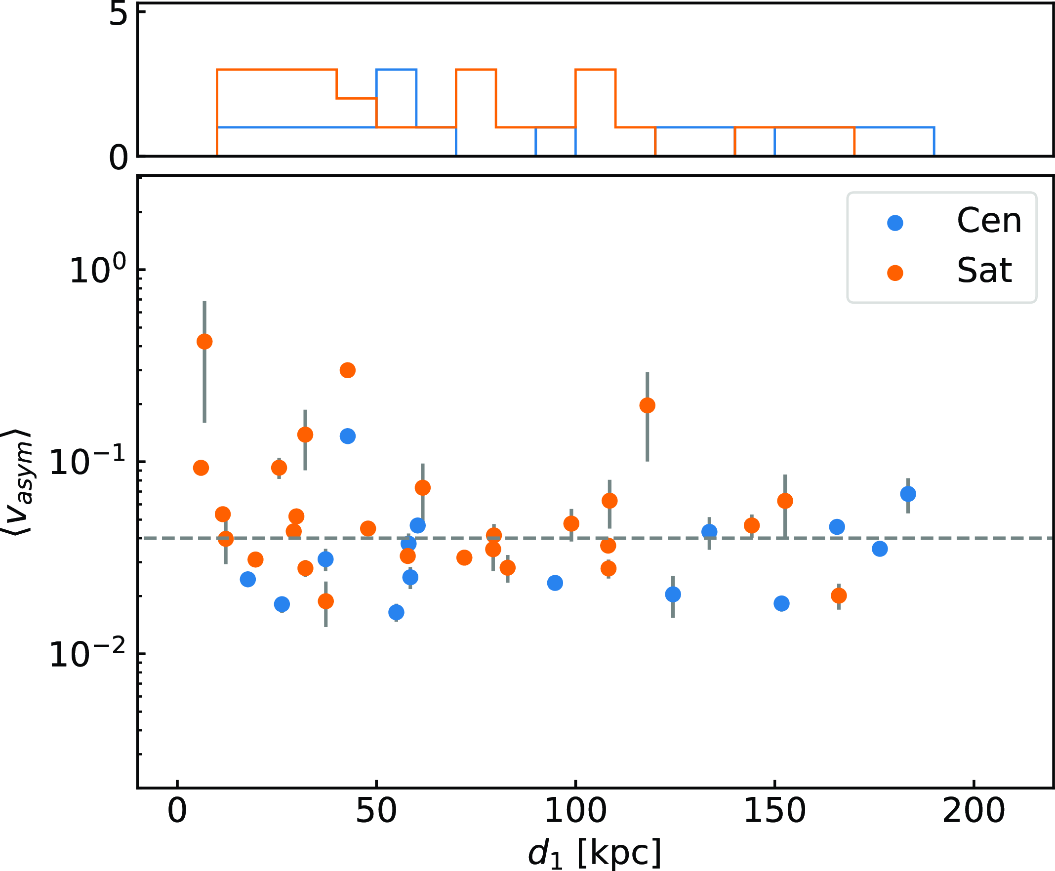
Figure 6.
 $\langle v_{asym} \rangle$
vs distance to the nearest neighbour,
$\langle v_{asym} \rangle$
vs distance to the nearest neighbour,
 $d_1$
where the points are coloured by whether they are a central (blue) or satellite (satellite) galaxy. The grey dashed line is the asymmetry cutoff. Galaxies are, on average, more asymmetric as the projected distance to the nearest neighbour decreases; however this is primarily found in satellite galaxies, not centrals. The histogram above shows the number of asymmetric central and satellite galaxies within the
$d_1$
where the points are coloured by whether they are a central (blue) or satellite (satellite) galaxy. The grey dashed line is the asymmetry cutoff. Galaxies are, on average, more asymmetric as the projected distance to the nearest neighbour decreases; however this is primarily found in satellite galaxies, not centrals. The histogram above shows the number of asymmetric central and satellite galaxies within the
 $d_1$
bins of 10 kpc.
$d_1$
bins of 10 kpc.
4.1.1 Projected distance to nearest neighbour
Having a large projected distance between galaxies is also a likely explanation for those groups with satellites that are symmetric, as they are probably further away (but still within linking distance) and are not interacting with the central. This can be seen in Fig. 6 where we plot
 $\langle v_{asym} \rangle$
against the co-moving projected distance to the nearest neighbouring galaxy. We see that the asymmetry increases as the projected distance decreases. This effect is more severe in satellite galaxies, where the fraction of asymmetric satellites increases as the projected distance decreases, whereas the fraction of asymmetric centrals stays roughly the same (see the histogram above Fig. 6). This is consistent with the findings in McElroy et al. (Reference McElroy2022) where the central galaxy became, and stayed asymmetric, after coalescence. It should also be said that McElroy et al. (Reference McElroy2022) investigate asymmetries in the stellar LOSVD, and not the ionised gas, as we have done in this work.
$\langle v_{asym} \rangle$
against the co-moving projected distance to the nearest neighbouring galaxy. We see that the asymmetry increases as the projected distance decreases. This effect is more severe in satellite galaxies, where the fraction of asymmetric satellites increases as the projected distance decreases, whereas the fraction of asymmetric centrals stays roughly the same (see the histogram above Fig. 6). This is consistent with the findings in McElroy et al. (Reference McElroy2022) where the central galaxy became, and stayed asymmetric, after coalescence. It should also be said that McElroy et al. (Reference McElroy2022) investigate asymmetries in the stellar LOSVD, and not the ionised gas, as we have done in this work.
Bloom et al. (Reference Bloom2018) used ionised gas kinematic asymmetries, as we have done in this work and found that the distance to the nearest neighbour had a stronger influence on the asymmetry, than the distance to the 5th neighbouring galaxy. Our results, alongside Bloom et al. (Reference Bloom2018), would suggest that the symmetric satellites and centrals with small projected distances have most likely not experienced their first pericenter passage, as was found in McElroy et al. (Reference McElroy2022).
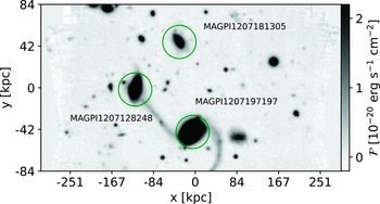
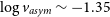
There is an example of one group consisting of two asymmetric satellites around a central galaxy. The group containing MAGPI1207197197, MAGPI1207128248, MAGPI1207181305 is a clearly interacting system with visible streams and tails connecting the individual galaxies (Fig. 7). This is consistent with findings in Feng et al. (Reference Feng, Shen, Yuan, Riffel and Pan2020) as the galaxies are clearly interacting with each other and are in close proximity (e.g., MAGPI1207197248 has a projected distance
 $\sim$
109 kpc and MAGPI1207181305 has a projected distanc
$\sim$
109 kpc and MAGPI1207181305 has a projected distanc
 $\sim$
138 kpc. Unfortunately, there were no other examples of all the galaxies in a single group being asymmetric, since not all of the galaxies within an individual group satisfied our selection criteria.
$\sim$
138 kpc. Unfortunately, there were no other examples of all the galaxies in a single group being asymmetric, since not all of the galaxies within an individual group satisfied our selection criteria.
Figure 7. A i-band cutout of the MAGPI1207 field, the three galaxies with green circles are MAGPI1207197197 (bottom right), MAGPI1207128248 (centre left), MAGPI1207181305 (above). Multiple other sources are in the field, but are unlabelled as they do not belong to the group featured. What is extremely noticeable is the presence of a tidal tail connecting MAGPI1207197197 and MAGPI1207128248 and the extremely extended, loosely wound spiral arm or a tidal tail.
4.1.2 Asymmetry in previous gas phase
We now hypothesise a scenario for the asymmetric outskirts we see in our sample. If we assume we are primarily tracing HII regions (i.e., formation of OB stars), we might expect that the ionised gas will retain some memory of its kinematic state from before it is ionised, when it was either atomic or molecular. It should be noted that ionised gas can also be found in a diffuse component (Diffuse Ionised Gas, DIG; Reynolds Reference Reynolds1990) since it is expected that DIG can account for as much as
 $\sim$
50 % of the H
$\sim$
50 % of the H
 $\alpha$
emission in galaxies (Oey et al. Reference Oey2007; Kreckel et al. Reference Kreckel2016). It is also likely that the surrounding DIG would also inherit the same kinematic state of the HII region since DIG is primarily from ionizing photons ‘leaking’ out of nearby HII regions with a mean free path of
$\alpha$
emission in galaxies (Oey et al. Reference Oey2007; Kreckel et al. Reference Kreckel2016). It is also likely that the surrounding DIG would also inherit the same kinematic state of the HII region since DIG is primarily from ionizing photons ‘leaking’ out of nearby HII regions with a mean free path of
 $\sim$
2 kpc (Belfiore et al. Reference Belfiore2022). Gas can be ionised through physical processes other than star formation (e.g., AGN, shocks), we discuss these in the Section 4.2.
$\sim$
2 kpc (Belfiore et al. Reference Belfiore2022). Gas can be ionised through physical processes other than star formation (e.g., AGN, shocks), we discuss these in the Section 4.2.
The now ionised gas would not move far from where it was when it was in the previous phase, due to the near-instantaneous snapshot the H
 $\alpha$
line provides; meaning that that the asymmetry we observed in the ionised gas may reflect that of the previous atomic or molecular gas phase. The now ionised gas would maintain the same kinematic disturbance from its previous phase. Having asymmetric outskirts in the ionised gas would be consistent if it was actually due to the HI becoming disturbed first, either from ram-pressure stripping or interactions. Findings of disturbed morphologies and kinematics for HI, CO (tracing molecular gas) and spatially coinciding H
$\alpha$
line provides; meaning that that the asymmetry we observed in the ionised gas may reflect that of the previous atomic or molecular gas phase. The now ionised gas would maintain the same kinematic disturbance from its previous phase. Having asymmetric outskirts in the ionised gas would be consistent if it was actually due to the HI becoming disturbed first, either from ram-pressure stripping or interactions. Findings of disturbed morphologies and kinematics for HI, CO (tracing molecular gas) and spatially coinciding H
 $\alpha$
‘blobs’ lends support for a galaxy’s environment being responsible for the disturbed kinematics in the ionised gas (Lee et al. Reference Lee2017; Choi, Kim, & Chung Reference Choi, Kim and Chung2022).
$\alpha$
‘blobs’ lends support for a galaxy’s environment being responsible for the disturbed kinematics in the ionised gas (Lee et al. Reference Lee2017; Choi, Kim, & Chung Reference Choi, Kim and Chung2022).
It should be said that this is only true if the HI ends up closer to optical disk after the environmental interaction, due to HI reaching a larger radial extent compared to the molecular and ionised gas. Though recent studies have found that the environment can impact HI within the HI truncation radius,
 $R_\mathrm{HI}$
, as environmental stripping lowers the HI gas surface density of the entire galaxy (Watts et al. Reference Watts2023b). It seems reasonable that a decreasing gas surface density (i.e., a redistribution of the gas) would be accompanied by a kinematic disturbance.
$R_\mathrm{HI}$
, as environmental stripping lowers the HI gas surface density of the entire galaxy (Watts et al. Reference Watts2023b). It seems reasonable that a decreasing gas surface density (i.e., a redistribution of the gas) would be accompanied by a kinematic disturbance.
The relationship between the asymmetries in ionised and atomic phases was investigated more deeply in Watts et al. (Reference Watts2023a) where they report that the connection was more nuanced then initially thought. However, their analysis of asymmetry was restricted to global flux profiles, not asymmetries in velocity maps. Analysing global flux profiles would wash out all the asymmetries, which we find to localised to specific regions. Using kinemetry on resolved HI velocity maps may result in a stronger connection between the ionised gas and atomic phase.

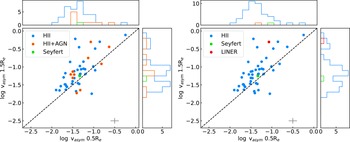
Figure 8.
Left: v
 $_{asym}$
(1.5R
$_{asym}$
(1.5R
 $_e$
) vs v
$_e$
) vs v
 $_{asym}$
(0.5R
$_{asym}$
(0.5R
 $_e$
) where the points are coloured according to the classification from Fig. 2. Right: The same are left, except the points are coloured by the classification according to the [SII]-BPT in Fig. 2. The dashed line is both is 1:1. The median error bars for the sample is shown in the bottom right corner. The histograms above and the side of each shows the distribution of v
$_e$
) where the points are coloured according to the classification from Fig. 2. Right: The same are left, except the points are coloured by the classification according to the [SII]-BPT in Fig. 2. The dashed line is both is 1:1. The median error bars for the sample is shown in the bottom right corner. The histograms above and the side of each shows the distribution of v
 $_{asym}$
of each ionisation source. Right: The same as left, except we use only the classification from [SII]-BPT. It is included to break the degeneracy between purely AGN and HII+AGN galaxies.
$_{asym}$
of each ionisation source. Right: The same as left, except we use only the classification from [SII]-BPT. It is included to break the degeneracy between purely AGN and HII+AGN galaxies.
4.2 Active galactic nuclei
Since
 $\sim$
29% of the galaxies in our sample host an AGN or HII+AGN ionisation, we can investigate if an AGN can explain galaxies with larger inner asymmetries compared to their outskirts. AGNs are proven essential for reproducing the high mass end of the observed stellar mass function by preventing hot halo gas from cooling, effectively stopping further star formation in massive galaxies (Silk & Rees Reference Silk and Rees1998; Bower et al. Reference Bower2006; Hopkins et al. Reference Hopkins2006; Schaye et al. Reference Schaye2015; Bower et al. Reference Bower2017). AGN are also often found in galaxies with disturbed kinematics (Greene et al. Reference Greene, Zakamska, Ho and Barth2011; Zakamska et al. Reference Zakamska2016; Ellison et al. Reference Ellison2019; Juneau et al. Reference Juneau2022). Being centrally located within the galaxy, we might expect that the asymmetry would be larger inside a galaxy than it is in the outskirts for a galaxy with an AGN. The nuclear region of an AGN galaxy can have a misaligned PA compared to their outskirts (e.g., Ilha et al. Reference Ilha2022; Ristea et al. Reference Ristea2022), this would cause larger asymmetries when performing kinemetry on nuclear regions.
$\sim$
29% of the galaxies in our sample host an AGN or HII+AGN ionisation, we can investigate if an AGN can explain galaxies with larger inner asymmetries compared to their outskirts. AGNs are proven essential for reproducing the high mass end of the observed stellar mass function by preventing hot halo gas from cooling, effectively stopping further star formation in massive galaxies (Silk & Rees Reference Silk and Rees1998; Bower et al. Reference Bower2006; Hopkins et al. Reference Hopkins2006; Schaye et al. Reference Schaye2015; Bower et al. Reference Bower2017). AGN are also often found in galaxies with disturbed kinematics (Greene et al. Reference Greene, Zakamska, Ho and Barth2011; Zakamska et al. Reference Zakamska2016; Ellison et al. Reference Ellison2019; Juneau et al. Reference Juneau2022). Being centrally located within the galaxy, we might expect that the asymmetry would be larger inside a galaxy than it is in the outskirts for a galaxy with an AGN. The nuclear region of an AGN galaxy can have a misaligned PA compared to their outskirts (e.g., Ilha et al. Reference Ilha2022; Ristea et al. Reference Ristea2022), this would cause larger asymmetries when performing kinemetry on nuclear regions.
There are caveats in our analysis with AGN and HII+AGN galaxies that should be mentioned before we discuss our results. First, the kinematic maps used in this analysis are constructed from a set of Gaussian fits to spectral lines where the width and relative velocity are tied to one line; H
 $\alpha$
for our redshift range. When we observe galaxies with HII+AGN ionised gas components, these are combined in the LOSVD. This can be an issue when fitting single component Gaussians to the spectra (Liu et al. Reference Liu, Zakamska, Greene, Nesvadba and Liu2013; Lena et al. Reference Lena2015; Fischer et al. Reference Fischer2017). This implies that the kinematic maps modelled may not be adequate in the nuclear region. Kinematic maps of the central regions that use multiple components might provide more informative kinematics of these regions, but fitting emission with multiple components is a complex problem that requires high spectral resolution, high signal-to-noise and adequate software, which is beyond the scope of this paper. It is also possible that the inner regions are unresolved for galaxies whose
$\alpha$
for our redshift range. When we observe galaxies with HII+AGN ionised gas components, these are combined in the LOSVD. This can be an issue when fitting single component Gaussians to the spectra (Liu et al. Reference Liu, Zakamska, Greene, Nesvadba and Liu2013; Lena et al. Reference Lena2015; Fischer et al. Reference Fischer2017). This implies that the kinematic maps modelled may not be adequate in the nuclear region. Kinematic maps of the central regions that use multiple components might provide more informative kinematics of these regions, but fitting emission with multiple components is a complex problem that requires high spectral resolution, high signal-to-noise and adequate software, which is beyond the scope of this paper. It is also possible that the inner regions are unresolved for galaxies whose
 $0.5R_e$
is only just larger than our spatial resolution cutoff, consequently the complex kinematic signatures would be smoothed out from resulting beam smearing. To mitigate these effects, AGN galaxies with poor GIST fits have been removed from this analysis (see Fig. 3 and the second last paragraph of Section 3), and we have only included those AGN galaxies where the uncertainties are no worse than expected for star-forming galaxies.
$0.5R_e$
is only just larger than our spatial resolution cutoff, consequently the complex kinematic signatures would be smoothed out from resulting beam smearing. To mitigate these effects, AGN galaxies with poor GIST fits have been removed from this analysis (see Fig. 3 and the second last paragraph of Section 3), and we have only included those AGN galaxies where the uncertainties are no worse than expected for star-forming galaxies.
The left panel of Fig. 8 shows
 $v_{\rm asym}$
(
$v_{\rm asym}$
(
 $0.5Re$
) vs
$0.5Re$
) vs
 $v_{\rm asym}$
(
$v_{\rm asym}$
(
 $1.5Re$
) for each classification across all three BPT diagrams in Fig. 2. The Seyfert galaxy and seven of the ten HII+AGN galaxies have
$1.5Re$
) for each classification across all three BPT diagrams in Fig. 2. The Seyfert galaxy and seven of the ten HII+AGN galaxies have
 $v_{\rm asym} (1.5R_e)>v_{\rm asym} (0.5R_e)$
. Using the [SII]-BPT can break some of the degeneracy between purely AGN and HII+AGN (e.g., Kewley et al. Reference Kewley, Groves, Kauffmann and Heckman2006). To that end, we investigate the same
$v_{\rm asym} (1.5R_e)>v_{\rm asym} (0.5R_e)$
. Using the [SII]-BPT can break some of the degeneracy between purely AGN and HII+AGN (e.g., Kewley et al. Reference Kewley, Groves, Kauffmann and Heckman2006). To that end, we investigate the same
 $v_{\rm asym}$
(
$v_{\rm asym}$
(
 $0.5Re$
) vs
$0.5Re$
) vs
 $v_{\rm asym}$
(
$v_{\rm asym}$
(
 $1.5Re$
) parameter space using the classification from the [SII]-BPT diagram (see right panel of Fig. 8). Although there are only two confirmed AGNs using [SII]-BPT, both have larger asymmetries at 1.5
$1.5Re$
) parameter space using the classification from the [SII]-BPT diagram (see right panel of Fig. 8). Although there are only two confirmed AGNs using [SII]-BPT, both have larger asymmetries at 1.5
 $R_e$
. Looking at the histograms above and to the right of the panels in Fig. 8, we see that those galaxies with AGN or HII+AGN have larger asymmetries on average than purely star-forming galaxies. This suggests that hosting an AGN is associated, on average, with larger kinematic asymmetries in both the inner and outer regions.
$R_e$
. Looking at the histograms above and to the right of the panels in Fig. 8, we see that those galaxies with AGN or HII+AGN have larger asymmetries on average than purely star-forming galaxies. This suggests that hosting an AGN is associated, on average, with larger kinematic asymmetries in both the inner and outer regions.
Our results contrast with those in Bloom et al. (Reference Bloom2017a), who found no evidence to suggest that an AGN was the cause of
 $v_{\rm asym}$
. They are, however, consistent with findings in HI-SAMI where there was a lack of a connection between the asymmetry measured from HI global flux distributions (which primarily traces asymmetries at larger radial extents) and the more centrally concentrated ionised gas which come from AGN (Watts et al. Reference Watts2023a). The impact of AGN have on velocity maps in simulated galaxies has shown that those with AGN demonstrated larger asymmetries, and that velocity maps of simulated galaxies where AGN feedback was not implemented were inconsistent with the asymmetric AGN galaxies in CALIFA (Florian et al. Reference Florian2020).
$v_{\rm asym}$
. They are, however, consistent with findings in HI-SAMI where there was a lack of a connection between the asymmetry measured from HI global flux distributions (which primarily traces asymmetries at larger radial extents) and the more centrally concentrated ionised gas which come from AGN (Watts et al. Reference Watts2023a). The impact of AGN have on velocity maps in simulated galaxies has shown that those with AGN demonstrated larger asymmetries, and that velocity maps of simulated galaxies where AGN feedback was not implemented were inconsistent with the asymmetric AGN galaxies in CALIFA (Florian et al. Reference Florian2020).
It is hard to draw conclusions given the small number of confirmed AGN galaxies in this study (one Seyfert and one LINER using the [SII]-BPT). Given that most of the non-star-forming galaxies are HII+AGN, it could be that AGN, or some other processes are creating shocks, rather than outflows, leading to kinematics disturbances in the ionised gas at 1.5
 $R_e$
(Zakamska & Greene Reference Zakamska and Greene2014; Belfiore et al. Reference Belfiore2016). However, if these AGN galaxies have outflow signatures present in their spectra, the kinematic disturbances are most likely due to the outflows from the AGN.
$R_e$
(Zakamska & Greene Reference Zakamska and Greene2014; Belfiore et al. Reference Belfiore2016). However, if these AGN galaxies have outflow signatures present in their spectra, the kinematic disturbances are most likely due to the outflows from the AGN.
4.3 Star-formation and stellar mass
In this section, we discuss the possible impact the star formation activity and stellar mass could have in driving the asymmetry in the galaxies in our sample.
4.3.1 Star formation
Since a large asymmetry value is a result of the galaxy displaying more non-circular motion relative to its rotational motion (characterised by
 $k_1$
), we can investigate if more non-circular motion results in less rotational support in the gas. Less rotational support, from the non-circular motions, in the gas would lead to more gas collapsing, and we might expect the now ionised gas to inherit the same non-circular motions. To characterise whether our galaxies are experiencing enhanced star-formation due to the asymmetry, we consider the Star Forming Main Sequence (SFMS, Fig. 9) to determine which galaxies are showing increased or decreased star-formation activity. The SFMS for MAGPI galaxies at
$k_1$
), we can investigate if more non-circular motion results in less rotational support in the gas. Less rotational support, from the non-circular motions, in the gas would lead to more gas collapsing, and we might expect the now ionised gas to inherit the same non-circular motions. To characterise whether our galaxies are experiencing enhanced star-formation due to the asymmetry, we consider the Star Forming Main Sequence (SFMS, Fig. 9) to determine which galaxies are showing increased or decreased star-formation activity. The SFMS for MAGPI galaxies at
 $z\sim0.35$
is given by
$z\sim0.35$
is given by
 $\log_{10}$
(SFR) = 0.712
$\log_{10}$
(SFR) = 0.712
 $\pm0.04\times\log_{10}$
(M
$\pm0.04\times\log_{10}$
(M
 $_*$
) −7.293
$_*$
) −7.293
 $\pm$
0.06 (see Mun et al. in preparation for more information). We adopt a conservative logarithmic difference between the estimated SFR and the SFMS of
$\pm$
0.06 (see Mun et al. in preparation for more information). We adopt a conservative logarithmic difference between the estimated SFR and the SFMS of
 $\Delta_{SFR}>$
0.5 for star-bursting galaxies, 0.5
$\Delta_{SFR}>$
0.5 for star-bursting galaxies, 0.5
 $>\Delta_{SFR}>$
−1 for main sequence galaxies, and
$>\Delta_{SFR}>$
−1 for main sequence galaxies, and
 $\Delta_{MS}<$
−1 for quenched galaxies. We find that there are three star bursting galaxies, and no quiescent galaxies.
$\Delta_{MS}<$
−1 for quenched galaxies. We find that there are three star bursting galaxies, and no quiescent galaxies.

Figure 9.
Left: Logarithmic distance from SFMS (
 $\Delta_{\rm SFR}$
) vs Stellar Mass for MAGPI galaxies. Asymmetric galaxies (e.g.,
$\Delta_{\rm SFR}$
) vs Stellar Mass for MAGPI galaxies. Asymmetric galaxies (e.g.,
 $v_{asym}>0.04$
) are coloured blue, whereas symmetric galaxies (
$v_{asym}>0.04$
) are coloured blue, whereas symmetric galaxies (
 $v_{asym}<0.04$
) are coloured orange. Right: The same as left except we now use the same methodology for calculating
$v_{asym}<0.04$
) are coloured orange. Right: The same as left except we now use the same methodology for calculating
 $v_{\rm asym}$
, and cuttoff as Bloom et al. (Reference Bloom2017a). Including even terms in the asymmetry measure leads to more asymmetric, main sequence galaxies.
$v_{\rm asym}$
, and cuttoff as Bloom et al. (Reference Bloom2017a). Including even terms in the asymmetry measure leads to more asymmetric, main sequence galaxies.
We find that only one of the three star-bursting galaxies in our sample is asymmetric. We find that at low stellar masses, main sequence galaxies in our sample tend to be more asymmetric than their high stellar mass counterparts (see the left panel of Fig. 9). This result is consistent with those found in the MaNGA survey (Feng et al. Reference Feng, Shen, Yuan, Riffel and Pan2020); which found that at low stellar mass (
 $\log$
(M
$\log$
(M
 $_*$
/M
$_*$
/M
 $_\odot$
) < 10) star-bursting and main sequence galaxies displayed larger values of asymmetry compared to quiescent galaxies; but at large stellar masses, quiescent galaxies were either more, or at least as asymmetric as star-bursting and main sequence galaxies. Since we do not have any quiescent galaxies in our sample, we do not comment on the asymmetry in quiescent galaxies.
$_\odot$
) < 10) star-bursting and main sequence galaxies displayed larger values of asymmetry compared to quiescent galaxies; but at large stellar masses, quiescent galaxies were either more, or at least as asymmetric as star-bursting and main sequence galaxies. Since we do not have any quiescent galaxies in our sample, we do not comment on the asymmetry in quiescent galaxies.
We also compare our results with those in Bloom et al. (Reference Bloom2017a). To do this we adopt their methodology; chiefly, the larger cutoff value in asymmetry (0.065 vs 0.04) and re-computing
 $\langle v_{\rm asym} \rangle$
using only odd terms, although we stress that these terms must be considered (see Appendix A). Using their cutoff and
$\langle v_{\rm asym} \rangle$
using only odd terms, although we stress that these terms must be considered (see Appendix A). Using their cutoff and
 $v_{asym}$
value, our results are consistent with Bloom et al. (Reference Bloom2017a). We again find that only one star-bursting galaxy is considered asymmetric, and the majority of our main sequence galaxies are symmetric (see right panel of Fig. 9). Comparing our results between the different methodologies would suggest that the inclusion of even terms increases the asymmetry in main sequence galaxies.
$v_{asym}$
value, our results are consistent with Bloom et al. (Reference Bloom2017a). We again find that only one star-bursting galaxy is considered asymmetric, and the majority of our main sequence galaxies are symmetric (see right panel of Fig. 9). Comparing our results between the different methodologies would suggest that the inclusion of even terms increases the asymmetry in main sequence galaxies.
There are some caveats for the comparisons between SAMI, MaNGA and MAGPI that must be mentioned; the sample size used in Bloom et al. (Reference Bloom2017a,b) and Feng et al. (Reference Feng, Shen, Yuan, Riffel and Pan2020) is much larger than ours (
 $\sim 350$
vs
$\sim 350$
vs
 $\sim 50$
) meaning our sample could be missing a number of asymmetric and symmetric galaxies at all stellar masses. MaNGA and SAMI also average over smaller radial extents to our sample (MaNGA integrates out to 1
$\sim 50$
) meaning our sample could be missing a number of asymmetric and symmetric galaxies at all stellar masses. MaNGA and SAMI also average over smaller radial extents to our sample (MaNGA integrates out to 1
 $R_e$
and SAMI only uses 3 ellipses for all galaxies, regardless of physical size). As we have shown in Appendix A
$R_e$
and SAMI only uses 3 ellipses for all galaxies, regardless of physical size). As we have shown in Appendix A
 $v_{\rm asym}$
will more often be larger at more extended radii, causing our asymmetry values to be larger. However, considering we use a luminosity weighted asymmetry which increases the weighting towards the brighter, inner regions where the asymmetry will be smaller, this should be a minor affect. Thus, even with these caveats we are confident that the differences between MaNGA, SAMI and MAGPI (i.e., more asymmetric galaxies at all stellar masses in MAGPI) are real. Whether this is evolution of kinematic disturbances due to MAGPI being at higher redshift, will require a further analysis that is beyond scope of this paper.
$v_{\rm asym}$
will more often be larger at more extended radii, causing our asymmetry values to be larger. However, considering we use a luminosity weighted asymmetry which increases the weighting towards the brighter, inner regions where the asymmetry will be smaller, this should be a minor affect. Thus, even with these caveats we are confident that the differences between MaNGA, SAMI and MAGPI (i.e., more asymmetric galaxies at all stellar masses in MAGPI) are real. Whether this is evolution of kinematic disturbances due to MAGPI being at higher redshift, will require a further analysis that is beyond scope of this paper.
When finding the best fitting ellipse, kinemetry applies equal weighting to each spaxel along the ellipse, which essentially models a best-fitting ‘global’ ellipse for that radius. Occasionally, there will be differences between the ‘global’ model and the data that is not explained by the uncertainty in the velocity at that spaxel, implying these differences between the model and the data are located at a specific location within the galaxy; an example of this is shown in Fig. 10. Including more higher order terms (i.e., the even terms) allows kinemetry to ‘catch’ these local deviations from circular motion. Hence, these local deviations could be evidence of a local velocity disturbances (here we stress that this disturbance is different to the asymmetry, we are currently discussing). Since star formation is a local process, it becomes an obvious suspect for such a disturbance. Investigating the source of these disturbances will be done in subsequent work.

Figure 10. V
 $_{rot}$
as a function of azimuthal angle (
$_{rot}$
as a function of azimuthal angle (
 $\theta$
) around the ellipse for MAGPI1508197198.
$\theta$
) around the ellipse for MAGPI1508197198.
 $\Delta$
V are the residuals between the data and the model normalised to the maximum velocity of the galaxy. There are large (10s km s
$\Delta$
V are the residuals between the data and the model normalised to the maximum velocity of the galaxy. There are large (10s km s
 $^{-1}$
at
$^{-1}$
at
 $\theta$
=50 and
$\theta$
=50 and
 $\theta$
=90) differences between the model and data that are not explained by the errors in the velocity. These differences are localised to specific regions of the galaxy, hence could be the result of local physical processes (like star formation) causing disturbances.
$\theta$
=90) differences between the model and data that are not explained by the errors in the velocity. These differences are localised to specific regions of the galaxy, hence could be the result of local physical processes (like star formation) causing disturbances.

Figure 11.
Left:
 $\langle v_{\rm asym} \rangle$
vs stellar mass, Centre:
$\langle v_{\rm asym} \rangle$
vs stellar mass, Centre:
 $\langle v_{\rm asym} \rangle$
vs star formation rate, Right:
$\langle v_{\rm asym} \rangle$
vs star formation rate, Right:
 $\langle v_{\rm asym} \rangle$
vs
$\langle v_{\rm asym} \rangle$
vs
 $\Delta_{\rm SFR}$
. The
$\Delta_{\rm SFR}$
. The
 $\rho$
and p-values are calculated with respect to the
$\rho$
and p-values are calculated with respect to the
 $\langle v_{\rm asym}\rangle$
. HII+AGN galaxies are included in the left and right panel, but are excluded in the middle panel so as to investigate the relationship between purely star-forming galaxies. Including HII+AGN galaxies results in a considerably weaker correlation (
$\langle v_{\rm asym}\rangle$
. HII+AGN galaxies are included in the left and right panel, but are excluded in the middle panel so as to investigate the relationship between purely star-forming galaxies. Including HII+AGN galaxies results in a considerably weaker correlation (
 $\rho=-0.36,p=0.00124$
).
$\rho=-0.36,p=0.00124$
).
4.3.2 Stellar mass
The result for low stellar mass, main sequence galaxies being more asymmetric could be evidence of star-formation feedback disturbing the kinematics. Stellar feedback is predicted to be a prominent source of feedback in low stellar mass galaxies (Hopkins et al. Reference Hopkins2014, Reference Hopkins2018); stellar winds and SNe would cause disturbances in the ionised gas kinematics (assuming the ionisation is from hot OB stars) that could induce asymmetries. The conditions that regulate star formation operate on a large span of scales (Mpc to pc), though it is accepted to be a largely local process (Bigiel et al. Reference Bigiel2008; Kennicutt & Evans Reference Kennicutt and Evans2012, but see Bluck et al. Reference Bluck2020). Depending on the spatial distribution of star formation, it could be responsible for localised kinematic disturbances in the disk of galaxies.
A galaxy’s stellar mass correlates with its rotational velocity (i.e., The Tully-Fisher Relation; Tully & Fisher Reference Tully and Fisher1977), hence we expect the asymmetry to decrease with increasing stellar mass. In agreement with Bloom et al. (Reference Bloom2017a) and Feng et al. (Reference Feng, Shen, Yuan, Riffel and Pan2020), we find that there is a relatively weak anti-correlation between asymmetry and stellar mass as shown in Fig. 11. We find that the strength of the anti-correlation between asymmetry and stellar mass is not affected by whether we use
 $v_{\rm asym}$
at
$v_{\rm asym}$
at
 $0.5R_e$
(
$0.5R_e$
(
 $\rho = -0.41$
,
$\rho = -0.41$
,
 $p=0.00435$
),
$p=0.00435$
),
 $1.5R_e$
(
$1.5R_e$
(
 $\rho = -0.54$
,
$\rho = -0.54$
,
 $p=0.00005814$
) or
$p=0.00005814$
) or
 $\langle v_{\rm asym} \rangle$
(
$\langle v_{\rm asym} \rangle$
(
 $\rho = -0.48$
,
$\rho = -0.48$
,
 $p=0.000574$
).
$p=0.000574$
).
The absence of a strong anti-correlation with mass suggests that the connection between disturbed kinematics and a galaxy’s stellar mass is not as straightforward as initially suggested in Kannappan et al. (Reference Kannappan, Fabricant and Franx2002) and Cortese et al. (Reference Cortese2014). A galaxies’ SFR is strongly correlated with its stellar mass, and we find that
 $\langle v_{asym} \rangle$
has a stronger anti-correlation with SFR (
$\langle v_{asym} \rangle$
has a stronger anti-correlation with SFR (
 $\rho=-0.63,p=0.0000374$
) compared to stellar mass. A stronger anti-correlation could imply that the more non-circular motion the gas is exhibiting, the less gas is available for star-formation. Stellar/SNe feedback could be source for this non-circular motion/disturbed velocity, as we have discussed above.
$\rho=-0.63,p=0.0000374$
) compared to stellar mass. A stronger anti-correlation could imply that the more non-circular motion the gas is exhibiting, the less gas is available for star-formation. Stellar/SNe feedback could be source for this non-circular motion/disturbed velocity, as we have discussed above.
Our sample consists of star-forming galaxies with Sérsic indices
 $\sim$
1, which implies we are mostly looking at late-type galaxies. Late-type galaxies often host non-axisymmetric features such as bars (Kormendy & Kennicutt Reference Kormendy and Kennicutt2004; Cheung et al. Reference Cheung2013). Bars can cause gaseous inflows onto the nucleus of the galaxies, and these inflows would cause complex kinematics, particularly so for the inner regions. López-Cobá et al. (Reference López-Cobá2022) used a similar method to kinemetry to compute circular rotating models of barred galaxies that allowed for non-circular motions. They found evidence of velocity disturbances (characterised by higher-order Fourier coefficents) being caused by a non-axisymmetrical potential primarily in the inner regions where the bar is dominant; and although there is very little gas in bars, they still had a noticeable effect on the ionised gas kinematics. It seems reasonable that a bar would be effective source for complex inner kinematics. Future work will be done to identify asymmetric galaxies with bars based on MAGPI’s morphological classification (Foster et al., in preparation).
$\sim$
1, which implies we are mostly looking at late-type galaxies. Late-type galaxies often host non-axisymmetric features such as bars (Kormendy & Kennicutt Reference Kormendy and Kennicutt2004; Cheung et al. Reference Cheung2013). Bars can cause gaseous inflows onto the nucleus of the galaxies, and these inflows would cause complex kinematics, particularly so for the inner regions. López-Cobá et al. (Reference López-Cobá2022) used a similar method to kinemetry to compute circular rotating models of barred galaxies that allowed for non-circular motions. They found evidence of velocity disturbances (characterised by higher-order Fourier coefficents) being caused by a non-axisymmetrical potential primarily in the inner regions where the bar is dominant; and although there is very little gas in bars, they still had a noticeable effect on the ionised gas kinematics. It seems reasonable that a bar would be effective source for complex inner kinematics. Future work will be done to identify asymmetric galaxies with bars based on MAGPI’s morphological classification (Foster et al., in preparation).
5. Conclusions
We present a study of the kinematic asymmetries present in the ionised gas of a 47 star-forming galaxies (0.27
 $<z<$
0.35) from the MAGPI survey to study how the kinematic asymmetry changes between the inner regions (
$<z<$
0.35) from the MAGPI survey to study how the kinematic asymmetry changes between the inner regions (
 $0.5R_e$
) and outer regions (
$0.5R_e$
) and outer regions (
 $1.5R_e$
) of galaxies. We do this by fitting a series of ellipses to the line-of-sight velocity field using kinemetry and we quantify the asymmetry using similar practices in the literature. We investigate the different physical properties, in particular the environment, AGN, star formation activity, and stellar mass of our sample to find possible sources of the asymmetry in the velocity fields.
$1.5R_e$
) of galaxies. We do this by fitting a series of ellipses to the line-of-sight velocity field using kinemetry and we quantify the asymmetry using similar practices in the literature. We investigate the different physical properties, in particular the environment, AGN, star formation activity, and stellar mass of our sample to find possible sources of the asymmetry in the velocity fields.
Our findings are as follows:
-
• After testing three different models, we find that the kinematics are sufficiently complicated to warrant the inclusion of even terms in the fitted Fourier Series. We find that roughly 56% of our sample displays asymmetric velocity fields (
$\langle v_{\rm asym} \rangle > 0.04$
); while 81% displays larger asymmetry at
$1.5R_e$
compared to
$0.5R_e$
and 46% are asymmetric at both radial extents. The large fraction of galaxies with more disturbed outskirts is consistent with kinematics being largely driven by the gravitational potential, which would be significantly shallower in the outskirts compared to the inner regions, and so the asymmetry could be larger at a further galactocentric radius. -
• We find that most of our asymmetric galaxies belong in group environments (
$N_{gals}<6$
) where they would be affected by interactions from neighbouring galaxies. Focusing on the central galaxies, we find consistent results with interacting galaxies studied in simulations and previous studies using kinemetry, which found large asymmetries in interacting or merging galaxies. In line with other IFS surveys, we find that local environment, such as projected distance to nearest neighbour
$d_1$
, plays a role in whether a galaxy is asymmetric and that the most asymmetric galaxies tend to be satellites with small
$d_1$
. -
• We find no evidence to suggest that AGN confirmed with a BPT diagram within 1.5
$R_e$
preferentially drive inner asymmetries. The confirmed AGN hosts, as well as HII+AGN galaxies, demonstrate significant asymmetry at both probed radii, which suggests that outflows (if they are present) or shocks disrupts the kinematics across the whole galactic disk. A larger sample of confirmed AGN host galaxies is needed to better understand the effect of AGN on the asymmetry. -
• For our sample, asymmetric galaxies with low stellar masses (
$\log$
(M
$_*$
/M
$_\odot$
)
$<$
10) are preferentially found on the main sequence. We interpret this as possible evidence of stellar feedback driving the asymmetry in low stellar mass galaxies since stellar winds and SNe are primary sources of feedback in low stellar mass galaxies. -
• We find a negative trend between
$v_{\rm asym}$
and stellar mass, consistent with results from other IFS surveys. The negative trend persists, but does not increase in strength regardless whether
$v_{\rm asym}$
is measured at
$0.5R_e$
,
$1.5R_e$
or if we use a luminosity-weighted value. The negative trend between SFR and
$v_{asym}$
is stronger than what was found with stellar mass. We suggest that the weak trend is possibly due to a non-uniform distribution of mass or non-axisymmetric feature present in the optical disk, and that stellar feedback is responsible for the stronger anti-correlation with SFR.


Kinematic asymmetries provide an excellent probe into physical processes that govern galaxy evolution, but the connection between the two is, evidently, complex. We can leverage the higher lookback time of MAGPI against IFS surveys in the local Universe to investigate whether there is any evolution in these kinematic asymmetries. In future work, we plan to apply a consistent analytical framework across different surveys and investigate asymmetries across a range of lookback times.
Acknowledgement
We thank the referee for their constructive feedback on this manuscript draft. Based on observations collected at the European Organisation for Astronomical Research in the Southern Hemisphere under ESO program 1104.B-0536. We wish to thank the ESO staff, and in particular the staff at Paranal Observatory, for carrying out the MAGPI observations. MAGPI targets were selected from GAMA. GAMA is a joint European-Australasian project based around a spectroscopic campaign using the Anglo-Australian Telescope. GAMA is funded by the STFC (UK), the ARC (Australia), the AAO, and the participating institutions. GAMA photometry is based on observations made with ESO Telescopes at the La Silla Paranal Observatory under programme ID 179.A-2004, ID 177.A-3016. Part of this research was conducted by the Australian Research Council Centre of Excellence for All Sky Astrophysics in 3 Dimensions (ASTRO 3D), through project number CE170100013. CF is the recipient of an Australian Research Council Future Fellowship (project number FT210100168) funded by the Australian Government. CL, JTM and CF are the recipients of ARC Discovery Project DP210101945. EW acknowledges support by the Australian Research Council Centre of Excellence for All Sky Astrophysics in 3 Dimensions (ASTRO 3D), through project number CE170100013. LMV acknowledges support by the German Academic Scholarship Foundation (Studienstiftung des deutschen Volkes) and the COMPLEX project from the European Research Council (ERC) under the European Union’s Horizon 2020 research and innovation program grant agreement ERC-2019-AdG 882679. YP acknowledge National Science Foundation of China (NSFC) Grant No. 12125301, 12192220, 12192222, and the science research grants from the China Manned Space Project with No. CMS-CSST-2021-A07. PS is supported by Leiden University Oort Fellowship and the IAU Gruber Foundation Fellowship. This work makes use of colour scales chosen from van der Velden (Reference van der Velden2020).
Data Availability
The MAGPI spectral data underlying this work are available from the ESO Science Archive Facility (http://archive.eso.org/cms.html).
Appendix A. Quantifying Kinematic Asymmetry
This appendix contains a description of how we deal with artefacts in the data, the kinemetry models used, comparison between the models and various tests we employed to ensure we chose the best model for our analysis.
Numerical workaround for gaps in the kinematic maps
Our signal-to-noise cut sometimes rejects spaxels with otherwise valid neighbouring spaxels. These gaps cause the kinemetry algorithm to return trivial results for the corresponding radial ellipse, preventing a measure of the asymmetry at that radius and beyond even when data would otherwise allow. To mitigate this numerical artefact, we replace the velocity measurement of rejected spaxels with the median value from their eight adjacent spaxels to ensure we are not removing galaxies where we have kinematics out to our radii of interest (See Fig. A.1). Ellipses where we have thus replaced a significant fraction (more than 30%) of the spaxels along the ellipse with medians are exclude from further analysis. Hence, we can be sure that this numerical workaround does not leave a galaxy with poor kinemetry fits in our sample, and it does not remove a galaxy where we do indeed have a good fit.

Figure A.1.
Top Left: Velocity map for MAGPI1209197197 where we have masked the non-detected spaxels with median of the adjacent spaxels. Top Right: Velocity map for MAGPI1209197197 where we have masked non-detected spaxels and not replaced them with the median of adjacent spaxels. Middle Left: The fitted model from kinemetry from the velocity map in Top Left. Middle Right: The fitted model from kinemetry from the velocity map in Top Right. Bottom Left,
 $v_{asym}$
radial profiles from Middle Left. Bottom Right: The
$v_{asym}$
radial profiles from Middle Left. Bottom Right: The
 $v_{asym}$
radial profile from Middle Right. Notice that when non-detected spaxels are not replaced, the fitted model does not have coverage out to
$v_{asym}$
radial profile from Middle Right. Notice that when non-detected spaxels are not replaced, the fitted model does not have coverage out to
 $1.5R_e$
, and we do have
$1.5R_e$
, and we do have
 $v_{asym}$
values at
$v_{asym}$
values at
 $1.5R_e$
, even though we have kinematic information at that radial extent.
$1.5R_e$
, even though we have kinematic information at that radial extent.

Figure A.2. Rotational velocity (V
 $_{rot}$
, top) and residuals (bottom) as a function of azimuth around the ellipse with semi-major axis of 1.62′′ for MAGPI1527173209 (left) and MAGPI1209197197 (right). The orange line shows the expected values from a simple circular rotating model (i.e.,
$_{rot}$
, top) and residuals (bottom) as a function of azimuth around the ellipse with semi-major axis of 1.62′′ for MAGPI1527173209 (left) and MAGPI1209197197 (right). The orange line shows the expected values from a simple circular rotating model (i.e.,
 $B_1\cos(\theta)$
). The blue line is the fitted M2 model, which includes the higher order Fourier coefficients. Both velocity profiles can be adequately explained by M2. MAGPI1209197197 has a very symmetrical profile, whereas MAGPI1527173209 has asymmetric features that are not explained by the uncertainties (shown as error bars in the bottom panel), examples of which can be seen around
$B_1\cos(\theta)$
). The blue line is the fitted M2 model, which includes the higher order Fourier coefficients. Both velocity profiles can be adequately explained by M2. MAGPI1209197197 has a very symmetrical profile, whereas MAGPI1527173209 has asymmetric features that are not explained by the uncertainties (shown as error bars in the bottom panel), examples of which can be seen around
 $\theta$
= 100
$\theta$
= 100
 $^\circ$
and 300
$^\circ$
and 300
 $^\circ$
in the bottom left panel. Also note that these differences are an order of magnitude larger than those in the symmetric galaxy.
$^\circ$
in the bottom left panel. Also note that these differences are an order of magnitude larger than those in the symmetric galaxy.
Comparison between models
Krajnović et al. (Reference Krajnović2006) warned that adopting incorrect ellipse geometry (i.e. centre coordinates, PA and q) can result in additional power being distributed to other coefficients. In particular, an incorrect centre will cause
 $A_0, A_1, A_2, B_2, A_3$
and
$A_0, A_1, A_2, B_2, A_3$
and
 $A_4$
to have amplified values. This causes large, and in cases azimuthally periodic, residuals to appear between the data and the model that need to be considered in order to maintain a good fit to the data. This was noticed when running M1 on the MAGPI velocity maps, and motivated us to explore M2 and M3 as potential options.
$A_4$
to have amplified values. This causes large, and in cases azimuthally periodic, residuals to appear between the data and the model that need to be considered in order to maintain a good fit to the data. This was noticed when running M1 on the MAGPI velocity maps, and motivated us to explore M2 and M3 as potential options.

Figure A.3. Radial profiles of kinemetry coefficient from each model for galaxy MAGPI1205197197, a particularly well-resolved galaxy where we could fit 10 ellipses. The higher order coefficients, which have been normalised to
 $B_1$
, are plotted below. The left panel is M1, the middle panel is M2 and the right panel is M3. The grey dashed lines are
$B_1$
, are plotted below. The left panel is M1, the middle panel is M2 and the right panel is M3. The grey dashed lines are
 $\pm$
0.04 asymmetric limits commonly adopted in the literature. The solid grey line represent zero. Having a variable centre slightly decreases the
$\pm$
0.04 asymmetric limits commonly adopted in the literature. The solid grey line represent zero. Having a variable centre slightly decreases the
 $k_n$
values, whereas including even terms does not. The even terms are also a similar order of magnitude as the odd terms, and do not decrease the value of the odd terms.
$k_n$
values, whereas including even terms does not. The even terms are also a similar order of magnitude as the odd terms, and do not decrease the value of the odd terms.
Model 1: odd terms only, fixed centre
For all galaxies in our sample, we find a residual sinusoidal pattern with azimuth between our data and M1. An example of this sinusoidal residual pattern is shown in the left panel of Fig. A.2, where a significant and systematic difference is seen between the data and a simple circular rotating model as a function of azimuth. These periodic residuals imply that the model is unable to accommodate additional harmonic component(s) in the fitting. Due to these systematic residuals in M1, we do not use M1 in subsequent analyses.

Figure A.4. The fitted kinemetry ellipse from M1 (blue), M2 (orange) and M3 (green). The bottom panel shows the residuals from the fit, normalised to the maximum V
 $_{\rm rot}$
at that ellipse. The error bars shown are the errors on the velocities at those spaxels. The BIC values for the fitted ellipse are shown. Both M2 and M3 provide better fits to the data, suggesting that either an incorrect kinematic centre is being used, or even terms are required to ensure a good fit to the data.
$_{\rm rot}$
at that ellipse. The error bars shown are the errors on the velocities at those spaxels. The BIC values for the fitted ellipse are shown. Both M2 and M3 provide better fits to the data, suggesting that either an incorrect kinematic centre is being used, or even terms are required to ensure a good fit to the data.

Figure A.5. Histogram of the distance between the original centre (R
 $_i$
) coordinates and the final fitted centre (R
$_i$
) coordinates and the final fitted centre (R
 $_f$
) for M3. The median and mean are shown as maroon and green lines. The HWHM of the estimated PSF is shown in magenta. In most cases, the distance between initial and final coordinates is less the PSF. This implies that the the movement of the centre may not be physical, or at least we cannot be sure if its real at our current resolution limit.
$_f$
) for M3. The median and mean are shown as maroon and green lines. The HWHM of the estimated PSF is shown in magenta. In most cases, the distance between initial and final coordinates is less the PSF. This implies that the the movement of the centre may not be physical, or at least we cannot be sure if its real at our current resolution limit.

Figure A.6. Histogram of BIC values for the fitted kinemetry ellipse
 $1.5R_e$
for galaxies in our sample. The BIC values for M3 are consistently higher for every galaxy than both M1 and M2. Occasionally, M1 will have a larger BIC values than M2, indicating that M2 is better model, given our data.
$1.5R_e$
for galaxies in our sample. The BIC values for M3 are consistently higher for every galaxy than both M1 and M2. Occasionally, M1 will have a larger BIC values than M2, indicating that M2 is better model, given our data.
Model 3: odd terms only, variable centre
To determine which model is to be preferred between M2 and M3, we first determine if the power to the even terms in M2 is similar to that being distributed to the odd terms in M3. We do this by plotting radial profiles of each coefficient. Fig. A.3 shows radial value of each coefficients (
 $A_2,B_2, A_3$
etc…) for a typical galaxy in our sample. For most of the galaxies that are rotating as expected (i.e., low asymmetry), the power being distributed to the even terms is of similar magnitude to the odd terms at all radii. The galaxies that display large even coefficients in M2 also have large odd coefficients, and have very disturbed velocity maps (i.e., they would be considered asymmetric if we only used odd terms). The comparable magnitude of the even terms present in galaxies with regular velocity maps and disturbed velocity maps suggests that the even terms are, in fact, needed to adequately model not only the particularly disturbed velocity maps for our sample, but those galaxies which are rotating regularly as well. Including even terms, however, does not decrease the power being distributed to odd terms that could be affected by an incorrect ellipse geometry, suggesting that while it does improve the quality of the fit, it does not eliminate the amplification of
$A_2,B_2, A_3$
etc…) for a typical galaxy in our sample. For most of the galaxies that are rotating as expected (i.e., low asymmetry), the power being distributed to the even terms is of similar magnitude to the odd terms at all radii. The galaxies that display large even coefficients in M2 also have large odd coefficients, and have very disturbed velocity maps (i.e., they would be considered asymmetric if we only used odd terms). The comparable magnitude of the even terms present in galaxies with regular velocity maps and disturbed velocity maps suggests that the even terms are, in fact, needed to adequately model not only the particularly disturbed velocity maps for our sample, but those galaxies which are rotating regularly as well. Including even terms, however, does not decrease the power being distributed to odd terms that could be affected by an incorrect ellipse geometry, suggesting that while it does improve the quality of the fit, it does not eliminate the amplification of
 $A_1, A_3, B_3$
.
$A_1, A_3, B_3$
.
kinemetry, like most tilted-ring fitting algorithms, works with a degenerate parameter space, especially when allowing PA
 $_{\rm kin}$
,
$_{\rm kin}$
,
 $q_{\rm kin}$
and the centre coordinates to vary (Lelli, Fraternali, & Sancisi Reference Lelli, Fraternali and Sancisi2010; Di Teodoro & Fraternali Reference Di Teodoro and Fraternali2015). Fig. A.3 shows that allowing the centre’s coordinates to vary does decrease the power distributed to the odd terms (i.e.,
$q_{\rm kin}$
and the centre coordinates to vary (Lelli, Fraternali, & Sancisi Reference Lelli, Fraternali and Sancisi2010; Di Teodoro & Fraternali Reference Di Teodoro and Fraternali2015). Fig. A.3 shows that allowing the centre’s coordinates to vary does decrease the power distributed to the odd terms (i.e.,
 $A_1, A_3, B_3$
) and also improves the quality of the fit to the same level as the inclusion of even terms (i.e., residuals for M2 and M3 are similar). However, a variable kinematic centre could prove problematic if kinemetry begins to ‘overfit’ to the data. To gauge this, we calculate a Bayesian Information Criterion (BIC; Liddle Reference Liddle2007) for each ellipse. The BIC can be computed by
$A_1, A_3, B_3$
) and also improves the quality of the fit to the same level as the inclusion of even terms (i.e., residuals for M2 and M3 are similar). However, a variable kinematic centre could prove problematic if kinemetry begins to ‘overfit’ to the data. To gauge this, we calculate a Bayesian Information Criterion (BIC; Liddle Reference Liddle2007) for each ellipse. The BIC can be computed by
 \begin{equation} BIC = \chi^2 + k\ln N\end{equation}
where
 $\chi^2$
is the traditional chi-squared-goodness-of-fit value (or maximum liklihood with Gaussian errors, in a Bayesian context), k is the number of free parameters and N is the number of data used in the fitting. The advantage in using a BIC over a reduced
$\chi^2$
is the traditional chi-squared-goodness-of-fit value (or maximum liklihood with Gaussian errors, in a Bayesian context), k is the number of free parameters and N is the number of data used in the fitting. The advantage in using a BIC over a reduced
 $\chi^2$
is that unnecessary parameters are penalised. The middle and right-most panel in Fig. A.7 shows the 2D model velocity maps from M2 and M3. What kinemetry fits is a series of ellipses, and creates a 2D model by interpolating between ellipses. To see which model (M1, M2 or M3) is the best representation, given our data, we calculate the BIC value at
$\chi^2$
is that unnecessary parameters are penalised. The middle and right-most panel in Fig. A.7 shows the 2D model velocity maps from M2 and M3. What kinemetry fits is a series of ellipses, and creates a 2D model by interpolating between ellipses. To see which model (M1, M2 or M3) is the best representation, given our data, we calculate the BIC value at
 $1.5R_e$
, the same ellipse we use to exclude galaxies in Fig. 3. Fig. A.4 shows an example of an ellipse at
$1.5R_e$
, the same ellipse we use to exclude galaxies in Fig. 3. Fig. A.4 shows an example of an ellipse at
 $1.5R_e$
fitted with all three models. Both M2 and M3 remove the systematic residuals, but the BIC for M3 is much larger than M2. Fig. A.6 shows the distribution BIC values for galaxies in our sample. M3 consistently has larger BIC values than both M1 and M2, while occasionally M1 will have larger BIC values. This suggests that M3 overfits our data and is therefore not our preferred model.
$1.5R_e$
fitted with all three models. Both M2 and M3 remove the systematic residuals, but the BIC for M3 is much larger than M2. Fig. A.6 shows the distribution BIC values for galaxies in our sample. M3 consistently has larger BIC values than both M1 and M2, while occasionally M1 will have larger BIC values. This suggests that M3 overfits our data and is therefore not our preferred model.

Figure A.7. The velocity map, and fitted kinemetry models, for the asymmetric galaxy MAGPI1503208231. The left panel is the data, the middle panel is fitted model from M2, and the right most panel is the fitted model from M3. The black and white dots are the coordinates of the best-fitting centre. The red outline indicated the final ellipse’s centre coordinates. The magenta outline indicates the original coordinates. In most cases, the end coordinate returns sufficiently close to the original centre. It is important to notice that travelling kinematic centre hardly ever reaches distances larger than a PSF, suggesting that change is not physical meaningful. Moreover, the variable centre goes on a random walk around the original centre.
We also investigate where the variable kinematic centre travels on the map by calculating how far it travelled during the fitting routine. Fig. A.5 shows a histogram of the distance between the final centre coordinate and the initial centre coordinate
 $|R_f - R_i|$
. When we look at the distance the kinematic centre travels for M3, we find that the centre of most galaxies only moves roughly one spaxel (0.2 kpc) from the original coordinates with mean and median of 1.1 (1.42 kpc) and 0.96 (1.21 kpc) spaxels, respectively. At the maximum redshift of our sample (
$|R_f - R_i|$
. When we look at the distance the kinematic centre travels for M3, we find that the centre of most galaxies only moves roughly one spaxel (0.2 kpc) from the original coordinates with mean and median of 1.1 (1.42 kpc) and 0.96 (1.21 kpc) spaxels, respectively. At the maximum redshift of our sample (
 $z=0.35$
), the physical scale of the spatial PSF corresponds to
$z=0.35$
), the physical scale of the spatial PSF corresponds to
 $\sim$
3 kpc (1.65 spaxels). Of the 47 galaxies fitted with M3, only 4 have a greater maximum displacement than 3 kpc. Furthermore, in most cases, the kinematic centres return to the original coordinates as the number of spaxels fitted increases with radius (shown in Fig. A.7), suggesting that the centre displacement does not correspond to a real physical movement of the kinematic centre. Given our findings that allowing for varying kinematic centre seems to have a marginal effect on the position of the centre compared to the PSF, we do not continue to use M3.
$\sim$
3 kpc (1.65 spaxels). Of the 47 galaxies fitted with M3, only 4 have a greater maximum displacement than 3 kpc. Furthermore, in most cases, the kinematic centres return to the original coordinates as the number of spaxels fitted increases with radius (shown in Fig. A.7), suggesting that the centre displacement does not correspond to a real physical movement of the kinematic centre. Given our findings that allowing for varying kinematic centre seems to have a marginal effect on the position of the centre compared to the PSF, we do not continue to use M3.
Model 2: inclusion of even terms
Including even terms could cause the asymmetry to be inflated by virtue of including additional components in the sum in Equation (5). To investigate this, we split
 $v_{\rm asym}$
in its even and odd components using the equations below,
$v_{\rm asym}$
in its even and odd components using the equations below,
 \begin{equation} v_{\rm asym,even}=\frac{k_2+k_4}{2k_1}, \end{equation}
 \begin{equation} v_{\rm asym,odd}=\frac{k_3+k_5}{2k_1}. \end{equation}
The odd and even contributions are shown in Fig. A.8. We find that for small values of asymmetry (
 $v_{\rm asym,odd}$
,
$v_{\rm asym,odd}$
,
 $v_{\rm asym,even}<0.04,$
i.e., low asymmetry) the even terms are comparable to the odd terms. The even terms appear particularly important at
$v_{\rm asym,even}<0.04,$
i.e., low asymmetry) the even terms are comparable to the odd terms. The even terms appear particularly important at
 $0.5R_e$
where they scatter above and below the 1:1 line. At
$0.5R_e$
where they scatter above and below the 1:1 line. At
 $1.5R_e$
, the odd terms dominate
$1.5R_e$
, the odd terms dominate
 $v_{\rm asym}$
, but still with a non-negligible component in the even terms (i.e., are still on the 1:1 line). We conclude that even terms are necessary to adequately fit our galaxy sample and must be included.
$v_{\rm asym}$
, but still with a non-negligible component in the even terms (i.e., are still on the 1:1 line). We conclude that even terms are necessary to adequately fit our galaxy sample and must be included.
After much deliberation and testing, we completed our analysis using M2.

Figure A.8. Comparison of the power to the even (
 $\frac{k_2+k_4}{2k_1}$
) vs. odd (
$\frac{k_2+k_4}{2k_1}$
) vs. odd (
 $\frac{k_3+k_5}{2k_1}$
) moments for M2. The black dot dashed line represents the one-to-one. For low values and within
$\frac{k_3+k_5}{2k_1}$
) moments for M2. The black dot dashed line represents the one-to-one. For low values and within
 $0.5R_e$
(blue symbols), even and odd terms display similar contributions to the asymmetry; however at
$0.5R_e$
(blue symbols), even and odd terms display similar contributions to the asymmetry; however at
 $1.5R_e$
(orange symbols), the odd terms dominate the asymmetry measure.
$1.5R_e$
(orange symbols), the odd terms dominate the asymmetry measure.