


1. Introduction
Young, nearby stars are of major interest to scientists as they can provide insight into stellar evolution, as well as planetary formation. The exoplanet host 51 Eridani has been an object of interest in the astronomical community for a number of years. 51 Eridani is a F0 spectral type, $V = 5.22$
mag star and has a binary pair companion, GJ 3305A,B (both M0 dwarfs). 51 Eridani and GJ 3305A,B have a separation of 66
$V = 5.22$
mag star and has a binary pair companion, GJ 3305A,B (both M0 dwarfs). 51 Eridani and GJ 3305A,B have a separation of 66 $^{\prime\prime}$
, or roughly 2 000 au, and the system components are co-moving together in a hierarchical relationship (Feigelson et al. Reference Feigelson, Lawson, Stark, Townsley and Garmire2006). The exoplanet, 51 Eri b, has a semi-major axis of
$^{\prime\prime}$
, or roughly 2 000 au, and the system components are co-moving together in a hierarchical relationship (Feigelson et al. Reference Feigelson, Lawson, Stark, Townsley and Garmire2006). The exoplanet, 51 Eri b, has a semi-major axis of $12^{+4}_{-2}$
au, an inclination of
$12^{+4}_{-2}$
au, an inclination of $133^{+14}_{-7}$
deg, an eccentricity of
$133^{+14}_{-7}$
deg, an eccentricity of $0.45^{+0.10}_{-0.15}$
, and an orbital period of
$0.45^{+0.10}_{-0.15}$
, and an orbital period of $32^{+17}_{-9}$
years, all determined by fits of SPHERE and GPI data by Maire et al. (Reference Maire2019).
$32^{+17}_{-9}$
years, all determined by fits of SPHERE and GPI data by Maire et al. (Reference Maire2019).
51 Eridani is a member of the $\beta$
Pictoris moving group (
$\beta$
Pictoris moving group ( $\beta PMG$
), which is one of the youngest and closest moving groups to Earth. Zuckerman et al. (Reference Zuckerman, Song, Bessell and Webb2001) determined that the
$\beta PMG$
), which is one of the youngest and closest moving groups to Earth. Zuckerman et al. (Reference Zuckerman, Song, Bessell and Webb2001) determined that the $\beta$
Pictoris Moving Group consisted of 17 star systems. Since then, there are now a few hundred candidate systems belonging to the
$\beta$
Pictoris Moving Group consisted of 17 star systems. Since then, there are now a few hundred candidate systems belonging to the $\beta PMG$
(Miret-Roig et al. Reference Miret-Roig2020). The age estimates for the
$\beta PMG$
(Miret-Roig et al. Reference Miret-Roig2020). The age estimates for the $\beta PMG$
include
$\beta PMG$
include $23\pm3$
Myr (Mamajek and Bell Reference Mamajek and Bell2014) using the lithium depletion boundary method and isochronal ages for FGMK stars, which is consistent with the age estimate of 51 Eridani,
$23\pm3$
Myr (Mamajek and Bell Reference Mamajek and Bell2014) using the lithium depletion boundary method and isochronal ages for FGMK stars, which is consistent with the age estimate of 51 Eridani, $20 \pm 6$
Myr (Macintosh et al. Reference Macintosh2015) using the group’s lithium depletion boundary age. A more recent dynamical age estimate developed by Miret-Roig et al. (Reference Miret-Roig2020) presents an age of
$20 \pm 6$
Myr (Macintosh et al. Reference Macintosh2015) using the group’s lithium depletion boundary age. A more recent dynamical age estimate developed by Miret-Roig et al. (Reference Miret-Roig2020) presents an age of $18.5^{+2.0}_{-2.4}$
Myr. This estimate is a dynamical trace-back age that reconciles other trace-back estimates with other methods such as lithium depletion, isochronal ages, and other dynamical estimates.
$18.5^{+2.0}_{-2.4}$
Myr. This estimate is a dynamical trace-back age that reconciles other trace-back estimates with other methods such as lithium depletion, isochronal ages, and other dynamical estimates.
Macintosh et al. (Reference Macintosh2015) presented the discovery of the directly imaged planet 51 Eri b by the Gemini Planet Imager (GPI). Follow-up work by GPI and NIRC2 at the W. M. Keck 2 telescope (Wizinowich et al. Reference Wizinowich2000) have confirmed and refined the orbit and planetary properties of the system. The most current study of this system by Dupuy et al. (Reference Dupuy, Brandt and Brandt2022) determined an upper limit for the planet mass of $\geq 10.9$
M
$\geq 10.9$
M $_\mathrm{Jup}$
within a
$_\mathrm{Jup}$
within a $2 \sigma$
interval and an orbital separation of
$2 \sigma$
interval and an orbital separation of $10.4_{-1.1}^{+0.8}$
au derived using joint fitting of the Hipparcos-Gaia Catalog of Accelerations (HGCA-EDR3) proper motions and relative astrometry. Samland et al. (Reference Samland2017) determined a planetary effective temperature of
$10.4_{-1.1}^{+0.8}$
au derived using joint fitting of the Hipparcos-Gaia Catalog of Accelerations (HGCA-EDR3) proper motions and relative astrometry. Samland et al. (Reference Samland2017) determined a planetary effective temperature of $760\pm20$
K, and a radius of
$760\pm20$
K, and a radius of $1.1^{+0.2}_{-0.1}$
R
$1.1^{+0.2}_{-0.1}$
R $_\mathrm{Jup}$
from fitting spectro-photometry from VLT/SPHERE. Brown-Sevilla et al. (Reference Brown-Sevilla2023) recently published updated parameters on 51 Eri b using observations from VLT/SPHERE. A radiative transfer model fit using petitRADTRANS resulted in a planetary effective temperature of
$_\mathrm{Jup}$
from fitting spectro-photometry from VLT/SPHERE. Brown-Sevilla et al. (Reference Brown-Sevilla2023) recently published updated parameters on 51 Eri b using observations from VLT/SPHERE. A radiative transfer model fit using petitRADTRANS resulted in a planetary effective temperature of $807 \pm 45 $
K along with a radius of
$807 \pm 45 $
K along with a radius of $0.93 \pm 0.04$
R
$0.93 \pm 0.04$
R $_\mathrm{Jup}$
and a mass of
$_\mathrm{Jup}$
and a mass of $3.9 \pm 0.4$
M
$3.9 \pm 0.4$
M $_\mathrm{Jup}$
. For the mass of the planet, Brown-Sevilla et al. (Reference Brown-Sevilla2023) reported three possible masses:
$_\mathrm{Jup}$
. For the mass of the planet, Brown-Sevilla et al. (Reference Brown-Sevilla2023) reported three possible masses: $3.9\pm 0.4$
M
$3.9\pm 0.4$
M $_\mathrm{Jup}$
as the nominal result,
$_\mathrm{Jup}$
as the nominal result, $2.4$
M
$2.4$
M $_\mathrm{Jup}$
as a mass using evolutionary models by Baraffe et al. (Reference Baraffe, Chabrier, Allard and Hauschildt2002) with an age of 10 Myr, and
$_\mathrm{Jup}$
as a mass using evolutionary models by Baraffe et al. (Reference Baraffe, Chabrier, Allard and Hauschildt2002) with an age of 10 Myr, and $2.6$
M
$2.6$
M $_\mathrm{Jup}$
with an age of 20 Myr. These ages were taken from age estimates published by Lee et al. (Reference Lee, Song and Murphy2022) and Macintosh et al. (Reference Macintosh2015), respectively.
$_\mathrm{Jup}$
with an age of 20 Myr. These ages were taken from age estimates published by Lee et al. (Reference Lee, Song and Murphy2022) and Macintosh et al. (Reference Macintosh2015), respectively.
Given the young age of the system (both star and planet) determined by several literature sources, 51 Eri b is a perfect candidate to study a planet that is both young and still being influenced by its initial conditions of formation (Macintosh et al. Reference Macintosh2015). There are two main planet formation scenarios that most planets discovered fit into: the cold-start model and the hot-start model. The cold-start model is described by core accretion and usually results in lower entropy and a smaller radius of the planet. The hot-start model is described by disc instability which results in a planet with a higher entropy, a higher effective temperature, and a larger radius (Spiegel and Burrows Reference Spiegel and Burrows2012
a). A third formation scenario, cleverly named the warm-start model, involves a combination of the hot- and cold-start formation criteria (Spiegel and Burrows Reference Spiegel and Burrows2012
b). The warm-start model is a spectrum of initial conditions motivated by the observed preference of core accretion with gas giants forming closer to their stars and the recent observations of young exoplanets that are hotter than the cold-start model predictions but colder than the hot-start model predictions (Spiegel and Burrows Reference Spiegel and Burrows2012
b). A planet’s luminosity can provide insights into its formation because it is a function of age, mass, and initial conditions (Marley et al. Reference Marley, Fortney, Hubickyj, Bodenheimer and Lissauer2007; Spiegel and Burrows Reference Spiegel and Burrows2012
a). Macintosh et al. (Reference Macintosh2015)’s initial observations and study of 51 Eri b noted that the core accretion theory explains the formation of this planet due to the derived low luminosity range (log( $L/\mathrm{L}_{\odot}) = -5.4\,\mathrm{to} -5.8$
). Samland et al. (Reference Samland2017) explored all three scenarios and ruled out the cold-start models due to the new luminosity ranges (log(
$L/\mathrm{L}_{\odot}) = -5.4\,\mathrm{to} -5.8$
). Samland et al. (Reference Samland2017) explored all three scenarios and ruled out the cold-start models due to the new luminosity ranges (log( $L/\mathrm{L}_{\odot}) = -5.4\,\mathrm{to} -5.5$
) derived and found that the planet mass favoured the hot- or warm-start models. Dupuy et al. (Reference Dupuy, Brandt and Brandt2022) also ruled out the cold-start formation with their derivation of a lower limit on the initial specific entropy. Further study of this planet and its star can continue to explain its formation.
$L/\mathrm{L}_{\odot}) = -5.4\,\mathrm{to} -5.5$
) derived and found that the planet mass favoured the hot- or warm-start models. Dupuy et al. (Reference Dupuy, Brandt and Brandt2022) also ruled out the cold-start formation with their derivation of a lower limit on the initial specific entropy. Further study of this planet and its star can continue to explain its formation.
Characterising exoplanet host stars is key to understanding the exoplanet itself. The directly measured fundamental properties of a star, that is, radius, effective temperature, and luminosity, lead to more precise characterisation of the exoplanet. The habitable zone of a planet is heavily influenced by its host star, so in order to constrain the habitable zone boundaries and planets’ effective temperature, one must know the host star’s fundamental properties (von Braun and Boyajian Reference von Braun and Boyajian2017a). The derived age of a star from the directly measured fundamental properties can provide information about the formation of the exoplanet.
There are several indirect methods to determine stellar fundamental properties, such as atmospheric modelling and stellar evolutionary models. These models have been shown to have difficulties reproducing observations (Boyajian et al. Reference Boyajian2012, Reference Boyajian2013). Long baseline optical/infrared interferometry provides high angular resolution measurements of stars, allowing astronomers to calculate fundamental properties without relying on models.
Interferometric observations allow us to measure the stellar angular diameter, which when combined with the parallax, gives a direct measurement of the stellar radii, one of the fundamental parameters of an astronomical object. Optical interferometry achieves a higher resolution (on the order of milli-arcseconds) than most large telescopes by combining light from several pairs of telescopes that are separated across a variety of baselines, or the separation between telescopes. The resolution capability of an interferometer increases the precision of an angular diameter measurement which then lowers the uncertainty of stellar parameters that can be derived from the angular diameter, that is, stellar effective temperature and linear radius.
Similar to 51 Eridani and its planet, several other systems of stars with directly imaged exoplanets have been characterised with the CHARA Array. One such system is the $\kappa$
Andromedae and its exoplanet,
$\kappa$
Andromedae and its exoplanet, $\kappa$
And b by Jones et al. (Reference Jones, White, Quinn, Ireland, Boyajian, Schaefer and Baines2016). Jones et al. (Reference Jones, White, Quinn, Ireland, Boyajian, Schaefer and Baines2016) took into account the oblate nature and gravity darkening caused by
$\kappa$
And b by Jones et al. (Reference Jones, White, Quinn, Ireland, Boyajian, Schaefer and Baines2016). Jones et al. (Reference Jones, White, Quinn, Ireland, Boyajian, Schaefer and Baines2016) took into account the oblate nature and gravity darkening caused by $\kappa$
And’s rapid rotation through the use of modelling interferometric observations. The model results were used to determine fundamental stellar parameters, such as temperatures at the poles and equator, surface gravities, luminosity, stellar age and mass, and planetary age and mass.
$\kappa$
And’s rapid rotation through the use of modelling interferometric observations. The model results were used to determine fundamental stellar parameters, such as temperatures at the poles and equator, surface gravities, luminosity, stellar age and mass, and planetary age and mass.
Baines et al. (Reference Baines2012) used high-resolution interferometric observations to study HR 8799, which hosts four directly imaged companions (Marois et al. Reference Marois, Macintosh, Barman, Zuckerman, Song, Patience, Lafrenière and Doyon2008). The classification of the four companions, which is highly dependent on the age of the planet (inferred from the age of the star), is the subject of debate amongst astronomers (see Table 1 in Baines et al. Reference Baines2012). Baines et al. (Reference Baines2012) combined the angular diameter, parallax, and photometry to determine stellar parameters, such as linear radius, stellar effective temperature, and luminosity. The effective temperature calculated revealed two possible age scenarios of HR 8799: either the star is contracting onto the zero-age main sequence (ZAMS) or expanding away from it. Baines et al. (Reference Baines2012) used the Yonsei-Yale evolutionary models to investigate both possibilities. The resulting young ages (less than 0.1 Gyr) from either scenario highly favoured the classification of planet for the four companions, not brown dwarf. Additional recent works that use interferometric radii to determine planet properties are as follows but not limited to: Caballero et al. (Reference Caballero2022), Ellis et al. (Reference Ellis, Boyajian, von Braun, Ligi, Mourard, Dragomir, Schaefer and Farrington2021), and Ligi et al. (Reference Ligi2019) with more references tabulated in the von Braun and Boyajian (Reference von Braun and Boyajian2017 b) compilation. Other works demonstrating the wide utility of interferometric data are Korolik et al. (Reference Korolik2023) and Roettenbacher et al. (Reference Roettenbacher2022), which demonstrate analysing stellar activity and co-alignment of systems and Ibrahim et al. (Reference Ibrahim2023) which studies the inner au disc of Herbig Be star HD 190073.
In this paper, we present new stellar and planetary properties of the 51 Eridani system. This paper is organised as follows: the interferometric observations in Section 2, the directly determined stellar properties in Section 3, the derived stellar and planetary properties in Section 4, and a discussion of the results presented in this paper in comparison with the results published in the literature in Section 5.
2. Interferometric observations
The Center for High Angular Resolution Astronomy (CHARA) is a long baseline, optical/IR interferometer located at Mt. Wilson, CA. The CHARA Array (ten Brummelaar et al. Reference ten Brummelaar2005) comprises of six 1-metre telescopes arranged in a Y-shape configuration, with three arms: East (E), West (W), and South (S), each having two telescopes labeled 1 (outermost) and 2 (innermost). Baselines for the interferometer are formed by pairs of telescopes, such as E1/W1 (outermost East and West telescopes). We observed 51 Eridani in 2015 and 2016 using the Precision Astronomical Visible Observations (PAVO) beam combiner (Ireland et al. Reference Ireland, Schöller, Danchi and Delplancke2008), which measures interference fringes over a 630–950 nm dispersed bandwidth with two telescopes (as indicated in Table 1). We observed 51 Eridani in 2021 using the CLASSIC (Ten Brummelaar et al. Reference Ten Brummelaar2013) beam combiner, which operates in the near-infrared H-band.
Table 1. Summary of Observations: The date of observation in UT time is listed in the first column on the left. The wavelength of observation is shown in the second column. The baseline of observation is in the third column. The number of brackets is listed in the fourth column. The number in parentheses is the actual number of brackets used for data analysis due to the bad calibrators HD 29335 and HD 26912 (marked with a $^{*}$
in the table). Finally, the calibrators used for each night are listed in the right-most column.
$^{*}$
in the table). Finally, the calibrators used for each night are listed in the right-most column.
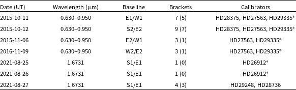
An observation sequence consists of the target star, or science star, and a selection of calibrator stars. Observations of calibrator stars allow for the removal of atmospheric and instrumentation noise from the observations of the science star. Data were taken in the following pattern: calibrator star – science star – calibrator star. This pattern is referred to as a bracket. The observations taken adhere to a minimum of two nights, two calibrators, and two baseline requirements to reduce and/or eliminate unknown systematic errors in the visibility data.
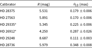
We use the Jean-Marie Mariotti Center Stellar Diameter Catalog (JSDC) (Chelli et al. Reference Chelli, Duvert, Bourgès, Mella, Lafrasse, Bonneau and Chesneau2016; Bourgés et al. Reference Bourgés, Lafrasse, Mella, Chesneau, Bouquin, Duvert, Chelli, Delfosse, Manset and Forshay2014)Footnote a to find suitable calibrator stars for our science target. The calibrator stars are chosen such that they are unresolved, nearby to the science star on the sky ( $<10^{\circ}$
), and have no known companions or rapid rotation. A summary of observations can be found in Table 1 and a list of calibrator stars used can be found in Table 2.
$<10^{\circ}$
), and have no known companions or rapid rotation. A summary of observations can be found in Table 1 and a list of calibrator stars used can be found in Table 2.
Table 2. Summary of calibrator stars: The R magnitudes and $\theta_\mathrm{LD}$
are taken from the JMMC Stellar Diameters Catalog v2 (Chelli et al. Reference Chelli, Duvert, Bourgès, Mella, Lafrasse, Bonneau and Chesneau2016). HD 29335 and HD 26912 are bad calibrators (marked with a
$\theta_\mathrm{LD}$
are taken from the JMMC Stellar Diameters Catalog v2 (Chelli et al. Reference Chelli, Duvert, Bourgès, Mella, Lafrasse, Bonneau and Chesneau2016). HD 29335 and HD 26912 are bad calibrators (marked with a $^{*}$
).
$^{*}$
).
We reduce and calibrate data for each night of PAVO observations using the PAVO software available through CHARA’s Remote Data Reduction Machine (Ireland et al. Reference Ireland, Schöller, Danchi and Delplancke2008). In the calibration process, we found that that the calibrator star, HD 29335, showed spurious results indicating that it was a bad calibrator. The amount of usable observations diminished after the removal of this calibrator from the observing sequence (seen in the parentheses in the column ‘Brackets’ in Table 1).
We reduce and calibrate data for each night of the CLASSIC observations using the CLASSIC/CLIMB reduction software redfluor, accessed through CHARA’s Remote Data Reduction Machine (ten Brummelaar Reference ten Brummelaar2014a,Reference ten Brummelaarb). For the first two nights of observations, only one observation of the science star and one observation of a calibrator star were made. We found that the calibrator was more resolved than the science star. Due to this trend, we suspect that this calibrator (HD 26912) is a bad calibrator and did not use in our analysis.
3. Directly determined stellar properties
An interferometer produces interference fringes that allow us to measure two basic pieces of information: the amplitude of the fringes and the phase shift of the peaks. The amplitudes allow us to measure visibilities, which describe the fringe contrast of the interference pattern. The visibility of a star can tell us about the star’s size, shape, and any surface features. Normalised visibilities are measured between 0 and 1, with a visibility of 0 indicating a completely resolved star and a visibility of 1 indicating a completely unresolved star.
When observing a star, it is important to remember that a star’s brightness is not uniform across the star. Optical depth and effective temperature gradients across the disc of a star combine to create an effect called limb darkening. To an observer, a star is brighter in the centre and then as you move out from the centre, the brightness goes down until it is 0 at the apparent edge of the star. A star’s uniform disc diameter does not take into account the limb darkening effect while the limb-darkened diameter does.
In order to determine the angular diameter of a star, the visibility squared as a function of baseline (B), angular diameter (either uniform, $\theta_\mathrm{UD}$
, or limb-darkened,
$\theta_\mathrm{UD}$
, or limb-darkened, $\theta_\mathrm{LD}$
), and wavelength (
$\theta_\mathrm{LD}$
), and wavelength ( $\lambda$
) is used to fit the interferometric visibilities using Equation (1):
$\lambda$
) is used to fit the interferometric visibilities using Equation (1):
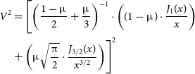 \begin{align} V^{2} & = \Biggl[\left(\frac{1-\unicode{x03BC}}{2} + \frac{\unicode{x03BC}}{3}\right)^{-1}\cdot\left((1-\unicode{x03BC}) \cdot \frac{J_{1}(x)}{x}\right)\nonumber\\& + \left(\unicode{x03BC} \sqrt{\frac{\unicode{x03C0}}{2}} \cdot \frac{J_{3/2}(x)}{x^{3/2}}\right)\Biggr]^{2} \end{align}
where $x = \frac{\unicode{x03C0} B \theta}{\lambda}$
and
$x = \frac{\unicode{x03C0} B \theta}{\lambda}$
and $\unicode{x03BC}$
is the limb-darkening coefficient (LDC). The first iteration of this fit is applied using a
$\unicode{x03BC}$
is the limb-darkening coefficient (LDC). The first iteration of this fit is applied using a $\unicode{x03BC}$
value of 0, which corresponds to a uniform disc diameter,
$\unicode{x03BC}$
value of 0, which corresponds to a uniform disc diameter, $\theta_\mathrm{ UD}$
.
$\theta_\mathrm{ UD}$
.
To estimate the bolometric flux ( $F_\mathrm{bol}$
) of 51 Eridani, we use the spectral energy distribution using available photometry from Gaia (Gaia Collaboration Reference Collaboration2020; Lindegren et al. Reference Lindegren2021), the Two-Micron All-Sky Survey (2MASS; Skrutskie et al. Reference Skrutskie2006), Tycho-2 (Høg et al. Reference Høg2000), the Wide-field Infrared Survey Explorer (WISE; Cutri and et al. Reference Cutri2014), and the General Catalog of Photometric Data (GCPD; Mermilliod et al. Reference Mermilliod, Mermilliod and Hauck1997). We combine the spectrum of 51 Eridani from the STIS Next Generation Spectral Library (NGSL; Heap and Lindler Reference Heap, Lindler, Vallenari, Tantalo, Portinari and Moretti2007) (covering the near UV and optical) with one from Cool Stars library (Rayner et al. Reference Rayner, Cushing and Vacca2009) (covering the near-infrared), filling any additional gaps with a stellar atmosphere (Allard et al. Reference Allard, Homeier, Freytag, Johns-Krull, Browning and West2011). We scaled the combined spectrum to match the photometry, yielding an absolutely calibrated spectrum. The final fit is shown in Fig. 1, and our bolometric flux measurement is in Table 3. More details on this fitting procedure, including our treatment of systematic uncertainties in the photometry and spectra are given in Mann et al. (Reference Mann, Feiden, Gaidos, Boyajian and von Braun2015) and (Reference Mann2016).
$F_\mathrm{bol}$
) of 51 Eridani, we use the spectral energy distribution using available photometry from Gaia (Gaia Collaboration Reference Collaboration2020; Lindegren et al. Reference Lindegren2021), the Two-Micron All-Sky Survey (2MASS; Skrutskie et al. Reference Skrutskie2006), Tycho-2 (Høg et al. Reference Høg2000), the Wide-field Infrared Survey Explorer (WISE; Cutri and et al. Reference Cutri2014), and the General Catalog of Photometric Data (GCPD; Mermilliod et al. Reference Mermilliod, Mermilliod and Hauck1997). We combine the spectrum of 51 Eridani from the STIS Next Generation Spectral Library (NGSL; Heap and Lindler Reference Heap, Lindler, Vallenari, Tantalo, Portinari and Moretti2007) (covering the near UV and optical) with one from Cool Stars library (Rayner et al. Reference Rayner, Cushing and Vacca2009) (covering the near-infrared), filling any additional gaps with a stellar atmosphere (Allard et al. Reference Allard, Homeier, Freytag, Johns-Krull, Browning and West2011). We scaled the combined spectrum to match the photometry, yielding an absolutely calibrated spectrum. The final fit is shown in Fig. 1, and our bolometric flux measurement is in Table 3. More details on this fitting procedure, including our treatment of systematic uncertainties in the photometry and spectra are given in Mann et al. (Reference Mann, Feiden, Gaidos, Boyajian and von Braun2015) and (Reference Mann2016).
Table 3. Stellar and planetary parameters for 51 Eridani and 51 Eri b. Each property is listed in the left column, the corresponding value in the centre column, and the source for each property in the right column. We use $\mathrm{R}_{\odot} = 6.957 \times 10^{8}\, \textrm{m}$
and
$\mathrm{R}_{\odot} = 6.957 \times 10^{8}\, \textrm{m}$
and $\mathrm{L}_{\odot} = 3.846 \times 10^{33} \mathrm{\,erg\,}\mathrm{s}^{-1}$
.
$\mathrm{L}_{\odot} = 3.846 \times 10^{33} \mathrm{\,erg\,}\mathrm{s}^{-1}$
.
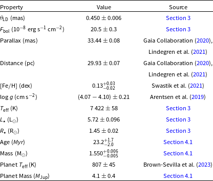
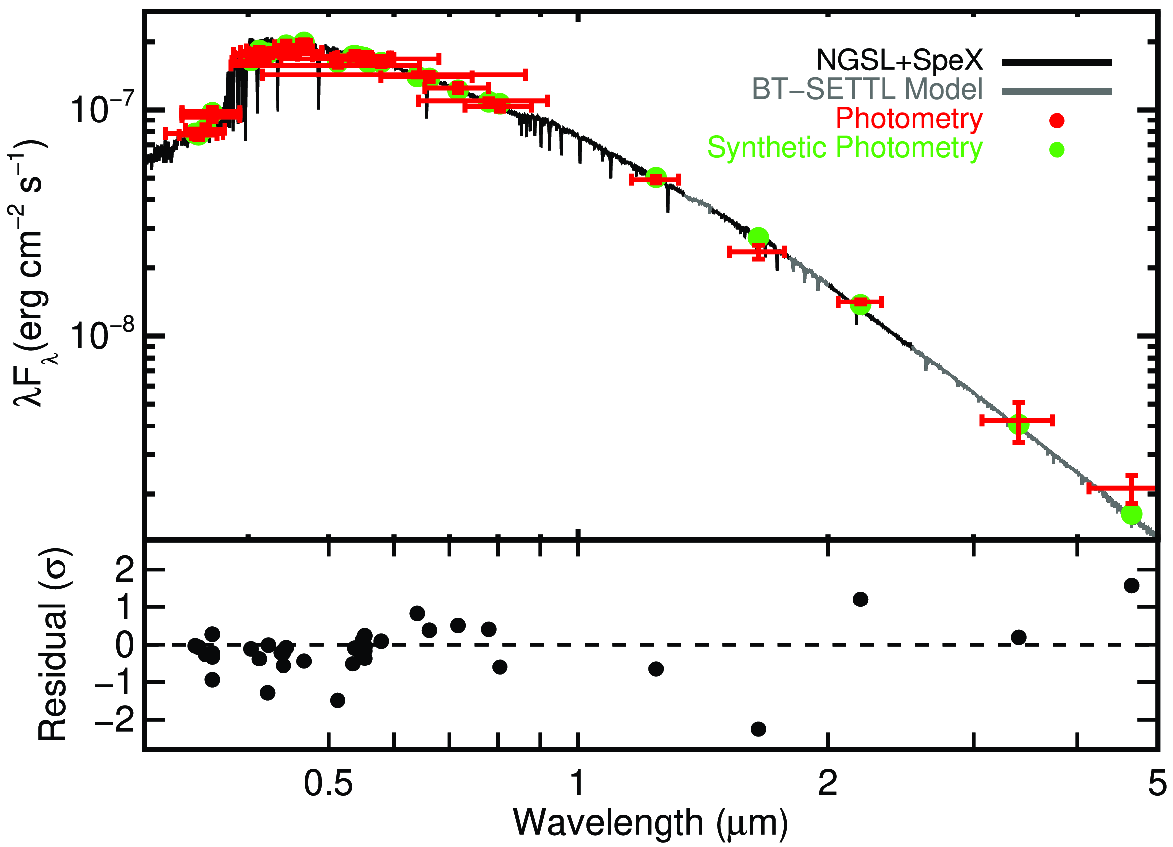
Figure 1. Spectral energy distribution and spectrum of 51 Eridani. The black line is the NGSL and SpeX spectrum, with grey regions indicating a model. Photometry is shown in red, with horizontal error bars indicating the width of the filter, while vertical show the photometric uncertainty. Synthetic photometry from the spectrum is shown in green. The bottom panel shows the difference between the spectrum and photometry in units of standard deviations.
From the angular diameter and $F_\mathrm{bol}$
, the stellar effective temperature,
$F_\mathrm{bol}$
, the stellar effective temperature, $T_\mathrm{eff}$
, is calculated using the following form of the Stefan–Boltzmann equation:
$T_\mathrm{eff}$
, is calculated using the following form of the Stefan–Boltzmann equation:
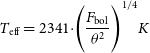 \begin{equation} T_\mathrm{eff} = 2341 \cdot \Biggr(\frac{F_\mathrm{bol}}{\theta^{2}} \Biggl)^{1/4} K \end{equation}
In Equation (2), the bolometric flux is in units of $10^{-8} \mathrm{\,erg\,}\mathrm{s}^{-1} \mathrm{cm}^{-2}$
and
$10^{-8} \mathrm{\,erg\,}\mathrm{s}^{-1} \mathrm{cm}^{-2}$
and $\theta$
is in units of mas. In the first initial calculation of
$\theta$
is in units of mas. In the first initial calculation of $T_\mathrm{eff}$
,
$T_\mathrm{eff}$
, $\theta_{UD}$
refers to the uniform disc angular diameter. In order to account for limb darkening, we use the Limb-Darkening Coefficients table (Claret and Bloemen Reference Claret and Bloemen2011) to solve for a linear R-band LDC with initial guesses of the star’s
$\theta_{UD}$
refers to the uniform disc angular diameter. In order to account for limb darkening, we use the Limb-Darkening Coefficients table (Claret and Bloemen Reference Claret and Bloemen2011) to solve for a linear R-band LDC with initial guesses of the star’s $T_\mathrm{eff}$
,
$T_\mathrm{eff}$
, $\log g$
, and [Fe/H]. This value is used in a subsequent
$\log g$
, and [Fe/H]. This value is used in a subsequent $\theta_\mathrm{LD}$
fit (Equation (1)) and a new temperature is derived using Equation (2) where
$\theta_\mathrm{LD}$
fit (Equation (1)) and a new temperature is derived using Equation (2) where $\theta$
is now referring to the limb-darkened angular diameter,
$\theta$
is now referring to the limb-darkened angular diameter, $\theta_\mathrm{ LD}$
. We iterate on this process twice when no changes are seen. We determine the error for
$\theta_\mathrm{ LD}$
. We iterate on this process twice when no changes are seen. We determine the error for $\theta_\mathrm{ LD}$
sampling the angular diameter in a Monte Carlo simulation, varying on a normal distribution of the uncertainties for wavelength (
$\theta_\mathrm{ LD}$
sampling the angular diameter in a Monte Carlo simulation, varying on a normal distribution of the uncertainties for wavelength ( $\pm5$
nm), calibrator diameters (5% of the diameter), and LDCs (
$\pm5$
nm), calibrator diameters (5% of the diameter), and LDCs ( $\pm 0.02$
). The resulting limb-darkened angular diameter is
$\pm 0.02$
). The resulting limb-darkened angular diameter is $\theta_\mathrm{LD} = 0.450 \pm 0.004$
mas.
$\theta_\mathrm{LD} = 0.450 \pm 0.004$
mas.
Systematic variations (i.e. due to atmospheric effects or instrument alignments) can occur between nights. To investigate any systematic variations, we solve for the angular diameter using the data for each night separately and found that they all agreed with $3\sigma$
of each other. We took a weighted average of the angular diameters from each individual night and found
$3\sigma$
of each other. We took a weighted average of the angular diameters from each individual night and found $\theta_\mathrm{LD} = 0.452 \pm 0.004$
mas, which agrees with the diameter from the combined fit within
$\theta_\mathrm{LD} = 0.452 \pm 0.004$
mas, which agrees with the diameter from the combined fit within $1\sigma$
. The weights for this average are
$1\sigma$
. The weights for this average are $\frac{1}{\sigma^{2}}$
where
$\frac{1}{\sigma^{2}}$
where $\sigma$
is the associated uncertainty for each data point. For the final limb-darkened angular diameter, we add the uncertainties from the combined diameter fit and the weighted average diameter in quadrature which can be found in Table 3.
$\sigma$
is the associated uncertainty for each data point. For the final limb-darkened angular diameter, we add the uncertainties from the combined diameter fit and the weighted average diameter in quadrature which can be found in Table 3.
Fig. 2 displays the PAVO binned and calibrated visibilities, the CLASSIC data and the final fit for angular diameter. The CLASSIC data presented are not used in the final fit for angular diameter because the observations do not adhere to the recommended observing minimum requirements of two nights, two calibrators, and two baselines (Boyajian et al. Reference Boyajian2012). The data shown in Fig. 2 are there to demonstrate where CLASSIC lies on the curve (see Section 5 for further discussion.)
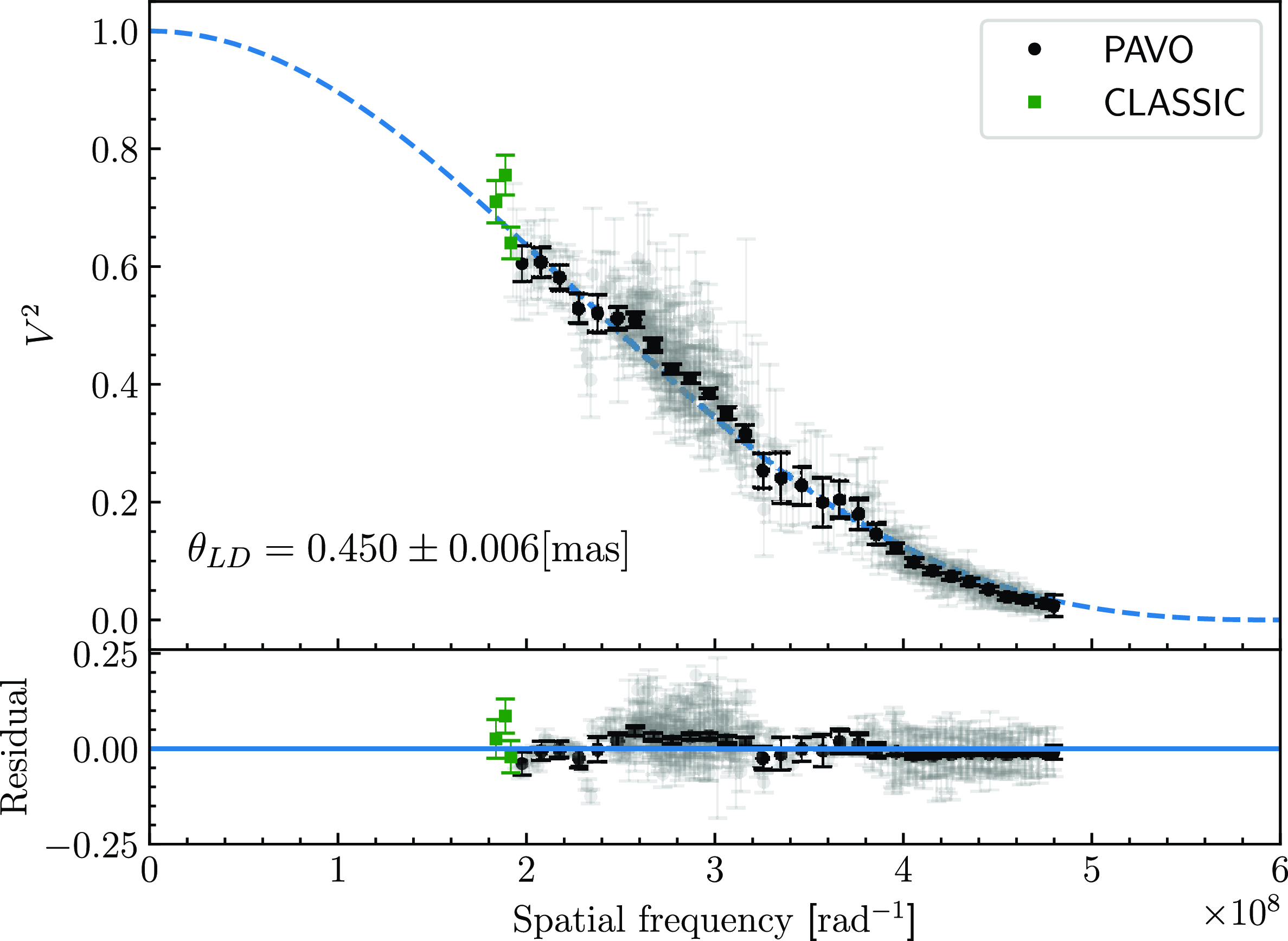
Figure 2. The top plot shows the calibrated squared visibilities and uncertainties from PAVO (in grey circles) and CLASSIC (in green squares). The PAVO data are binned in equal spacing, and the weighted average is shown (in black circles). The dashed blue line is the visibility model (Equation (1)) with the limb-darkened coefficient of $\unicode{x03BC} = 0.4516 \pm 0.0200$
. The bottom plot displays the residuals from PAVO (unbinned in grey and binned in black) and CLASSIC (in green).The limb-darkened angular diameter is
$\unicode{x03BC} = 0.4516 \pm 0.0200$
. The bottom plot displays the residuals from PAVO (unbinned in grey and binned in black) and CLASSIC (in green).The limb-darkened angular diameter is $0.450 \pm 0.006$
mas.
$0.450 \pm 0.006$
mas.
A stellar luminosity, $L_{\star}$
is calculated using Equation (3):
$L_{\star}$
is calculated using Equation (3):
 \begin{equation} L_{\star} = 4\unicode{x03C0} D^{2} F_\mathrm{bol} \end{equation}
where D is the distance (seen in Table 3) and $F_\mathrm{bol}$
is the bolometric flux (seen also in Table 3). The distance, D, is calculated using the zero-point corrected parallax,
$F_\mathrm{bol}$
is the bolometric flux (seen also in Table 3). The distance, D, is calculated using the zero-point corrected parallax, $33.44\pm 0.08$
mas (Gaia Collaboration Reference Collaboration2020; Lindegren et al. Reference Lindegren2021). This yields a distance of
$33.44\pm 0.08$
mas (Gaia Collaboration Reference Collaboration2020; Lindegren et al. Reference Lindegren2021). This yields a distance of $D = 29.93 \pm 0.07$
pc. The linear radius is then calculated using this new distance and Equation (4):
$D = 29.93 \pm 0.07$
pc. The linear radius is then calculated using this new distance and Equation (4):
 \begin{equation} R_{\star} = \frac{\theta_\mathrm{LD}\,D}{2} \end{equation}
where $\theta_\mathrm{LD}$
is the limb-darkened angular diameter and D is the zero-point corrected distance. The final parameters are presented in Table 3.
$\theta_\mathrm{LD}$
is the limb-darkened angular diameter and D is the zero-point corrected distance. The final parameters are presented in Table 3.
4. Modelled stellar and planetary properties
Using our measured effective temperature, luminosity, and radius, we estimate the age and mass of the star using stellar evolutionary models. Improved age estimates for the star means the age of the planet, 51 Eri b, is also improved given that the system is coeval. We then estimate the planet’s mass through evolutionary modelling and provide further insight on how the planet formed.
51 Eridani falls in a unique spot in the HR diagram. Previous works (summarised in the Introduction of Mamajek and Bell Reference Mamajek and Bell2014) indicated that the $\beta PMG$
consisted of pre-main sequence (PMS) stars. Mamajek and Bell (Reference Mamajek and Bell2014) analysed the kinematics of the
$\beta PMG$
consisted of pre-main sequence (PMS) stars. Mamajek and Bell (Reference Mamajek and Bell2014) analysed the kinematics of the $\beta PMG$
and concluded that the majority of the A0-F0 stars are either near or on the ZAMS, which includes 51 Eridani.
$\beta PMG$
and concluded that the majority of the A0-F0 stars are either near or on the ZAMS, which includes 51 Eridani.
4.1. Age and mass using isochronal modelling
To estimate the age and mass of 51 Eridani, we use stellar evolution models: the PAdova and TRieste Stellar Evolution Code (PARSEC) (Bressan et al. Reference Bressan, Marigo, Girardi, Salasnich, Dal Cero, Rubele and Nanni2012) and the Garching Stellar Evolution Code (GARSTEC) (Weiss and Schlattl Reference Weiss and Schlattl2008).
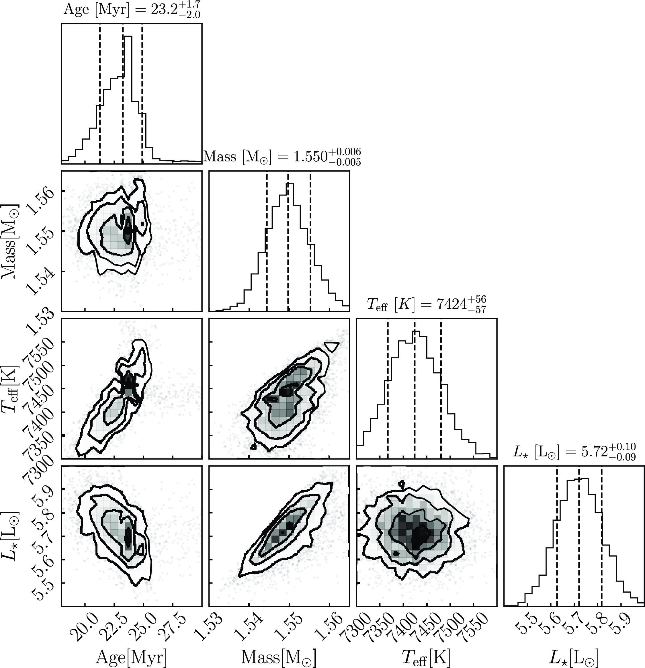
Figure 3. Corner plot for the PARSEC model displaying the results of a Monte Carlo simulation of 5 000 iterations to estimate the age and mass of 51 Eridani. The dashed vertical lines indicate the quantiles for each histogram: $16 \%$
, 50%, and 84% from left to right. The left-most line corresponds to the lower bound uncertainty. The middle line corresponds to the accepted value. The right-most line corresponds to the upper-bound uncertainty. The solutions are as follows: an age of
$16 \%$
, 50%, and 84% from left to right. The left-most line corresponds to the lower bound uncertainty. The middle line corresponds to the accepted value. The right-most line corresponds to the upper-bound uncertainty. The solutions are as follows: an age of $23.2^{+1.7}_{-2.0}$ $\mathrm{Myr}$
and a mass of
$\mathrm{Myr}$
and a mass of $1.550^{+0.006}_{-0.005}$
M
$1.550^{+0.006}_{-0.005}$
M $_{\odot}$
.
$_{\odot}$
.
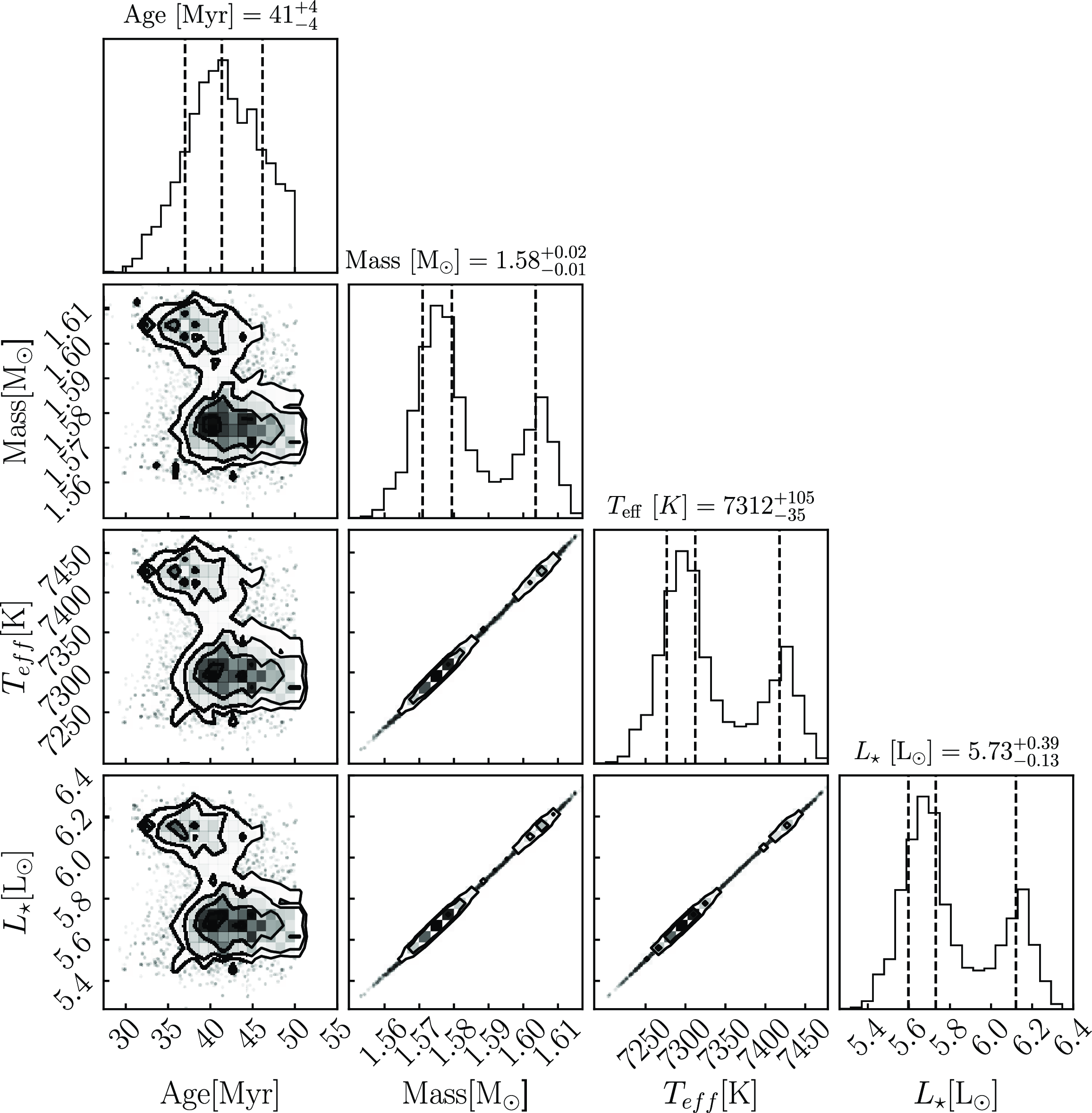
Figure 4. The above plot displays the corner plot for the GARSTEC model run through bagemass. The dashed vertical lines indicate the quantiles for each histogram: $16 \%$
, 50%, and 84% from left to right. The left-most line corresponds to the lower bound uncertainty. The middle line corresponds to the accepted value. The right-most line corresponds to the upper-bound uncertainty. The solutions are as follows: an age of
$16 \%$
, 50%, and 84% from left to right. The left-most line corresponds to the lower bound uncertainty. The middle line corresponds to the accepted value. The right-most line corresponds to the upper-bound uncertainty. The solutions are as follows: an age of $41\pm4$
Myr and a mass of
$41\pm4$
Myr and a mass of $1.58_{-0.01}^{+0.02}$
M
$1.58_{-0.01}^{+0.02}$
M $_{\odot}$
.
$_{\odot}$
.
We use the PARSEC version 1.2S modelFootnote b developed by Bressan et al. (Reference Bressan, Marigo, Girardi, Salasnich, Dal Cero, Rubele and Nanni2012) to create stellar isochrones given stellar priors. We generated isochrones for a range of ages between 0 and 50 Myr in steps of 0.5 Myrs in log space using a metal fraction of $Z = 0.0165$
(Table 3). We interpolated the outputted isochrones to obtain a finer grid of points along each isochrone track. We then performed two separate two-dimensional interpolations over
$Z = 0.0165$
(Table 3). We interpolated the outputted isochrones to obtain a finer grid of points along each isochrone track. We then performed two separate two-dimensional interpolations over $\log (L/\textit{L}_{\odot}$
) and
$\log (L/\textit{L}_{\odot}$
) and $T_\mathrm{eff}$
; one to extract an age and the other to extract a mass. We use a Monte Carlo simulation to obtain the errors for the age and mass estimates by sampling the
$T_\mathrm{eff}$
; one to extract an age and the other to extract a mass. We use a Monte Carlo simulation to obtain the errors for the age and mass estimates by sampling the $T_\mathrm{eff}$
and luminosity in a normal distribution. The posterior distributions are shown in Fig. 3. The final solution results in an age of
$T_\mathrm{eff}$
and luminosity in a normal distribution. The posterior distributions are shown in Fig. 3. The final solution results in an age of $23.2^{+1.7}_{-2.0}$
Myr and a mass of
$23.2^{+1.7}_{-2.0}$
Myr and a mass of $1.550^{+0.006}_{-0.005}$
M
$1.550^{+0.006}_{-0.005}$
M $_{\odot}$
.
$_{\odot}$
.
We then used the GARSTEC models (Weiss and Schlattl Reference Weiss and Schlattl2008) through the implementation of bagemass. bagemass (Maxted et al. Reference Maxted, Serenelli and Southworth2015) is a program written in Fortran that uses stellar evolution models to estimate the mass and age of a star and produces posterior probability distributions calculated using Bayesian methods. The GARSTEC model chosen has an $\alpha$
mixing length of 1.78 and a He-enhancement value of 0. The priors used are
$\alpha$
mixing length of 1.78 and a He-enhancement value of 0. The priors used are $T_\mathrm{eff}$
,
$T_\mathrm{eff}$
, $\log (L/\textit{L}_{\odot}$
), and [Fe/H] (Table 3). We fixed the metallicity and the age is given a range between 0 and 50 Myr. The posterior distributions are shown in Fig. 4. The final solution determined gives an age of
$\log (L/\textit{L}_{\odot}$
), and [Fe/H] (Table 3). We fixed the metallicity and the age is given a range between 0 and 50 Myr. The posterior distributions are shown in Fig. 4. The final solution determined gives an age of $41\pm 4$
Myr and a mass of
$41\pm 4$
Myr and a mass of $1.58_{-0.01}^{+0.02}$
M
$1.58_{-0.01}^{+0.02}$
M $_{\odot}$
.
$_{\odot}$
.
The age and mass estimates determined by the PARSEC model and the GARSTEC model are vastly different, with the GARSTEC model estimating an age almost twice that of the PARSEC model. The GARSTEC model could not return the prior distributions for $T_\mathrm{eff}$
and log(
$T_\mathrm{eff}$
and log( $L/\textit{L}_{\odot}$
) within the uncertainties or stay within the range of [Fe/H] priors given. Looking at the posterior distributions, we see that the GARSTEC model returns a bimodal solution and skews the priors, reflecting the model not returning the priors sufficiently well enough. This bimodal distribution could be due to the star’s location on the HR diagram. Although both models incorporate the PMS phase and the ZAMS phase of stellar evolution, the position of this star being right at the transition point could cause each model to either favour the PMS side or the early ZAMS side of this transition point. However, the PARSEC model is able to return the priors well and produce a single-mode solution. We adopt for the final results of this work, the PARSEC age and mass of
$L/\textit{L}_{\odot}$
) within the uncertainties or stay within the range of [Fe/H] priors given. Looking at the posterior distributions, we see that the GARSTEC model returns a bimodal solution and skews the priors, reflecting the model not returning the priors sufficiently well enough. This bimodal distribution could be due to the star’s location on the HR diagram. Although both models incorporate the PMS phase and the ZAMS phase of stellar evolution, the position of this star being right at the transition point could cause each model to either favour the PMS side or the early ZAMS side of this transition point. However, the PARSEC model is able to return the priors well and produce a single-mode solution. We adopt for the final results of this work, the PARSEC age and mass of $23.2^{+1.7}_{-2.0}$
Myr and
$23.2^{+1.7}_{-2.0}$
Myr and $1.550^{+0.006}_{-0.005}$
M
$1.550^{+0.006}_{-0.005}$
M $_{\odot}$
.
$_{\odot}$
.
The determination of age and mass is reliant on the priors of effective temperature and luminosity, so it is logical that the uncertainties of age and mass would be in turn reliant on these priors. In addition to the effect from temperature and luminosity, the uncertainties for age and mass are reliant on the choice in model chosen to determine these parameters (Tayar et al. Reference Tayar, Claytor, Huber and van Saders2022). The age is more affected by the choice in model, especially for stars closer to the ZAMS or PMS, where Tayar et al. (Reference Tayar, Claytor, Huber and van Saders2022) describes the differences in age being near 100% in these regions of parameter space. The differences between the PARSEC and the GARSTEC models used to estimate the age of 51 Eridani is another example of the discrepancy in age between models.
4.2 Analysis of the planetary companion 51 Eri b
The next step in the analysis of 51 Eri b is to estimate a mass using the assumption that the planet is the same age as the star (see Section 4.1). We use the Sonora Bobcat models (Marley et al. Reference Marley2021) which were developed to study L-, Y-, and T- type brown dwarfs and self-luminous exoplanets. 51 Eri b is considered to be a self-luminous planet, but it has been debated on whether 51 Eri b is an L- or T- type brown dwarf given its unique strong methane absorption features that are also seen in T-type brown dwarfs and similar near-IR colours to L-type brown dwarfs (Macintosh et al. Reference Macintosh2015).
The Sonora Bobcat models produce evolutionary tables that hold either age, mass, or bolometric luminosity fixed. For this paper’s purpose, we use the model holding mass fixed. In our analysis, we use the planet’s effective temperature of $T_\mathrm{eff} = 807 \pm 45 $
K (Brown-Sevilla et al. Reference Brown-Sevilla2023). Fig. 5 shows the Sonora Bobcat models as age vs.
$T_\mathrm{eff} = 807 \pm 45 $
K (Brown-Sevilla et al. Reference Brown-Sevilla2023). Fig. 5 shows the Sonora Bobcat models as age vs. $T_\mathrm{eff}$
along with the position of 51 Eri b. To determine a mass, we first perform a one-dimensional interpolation to create a finer grid of points for each of the iso-mass lines. We then perform an additional two-dimensional interpolation over the effective temperature and age and find the corresponding mass. To obtain uncertainties for the mass, we ran a Monte Carlo simulation, sampling the age and
$T_\mathrm{eff}$
along with the position of 51 Eri b. To determine a mass, we first perform a one-dimensional interpolation to create a finer grid of points for each of the iso-mass lines. We then perform an additional two-dimensional interpolation over the effective temperature and age and find the corresponding mass. To obtain uncertainties for the mass, we ran a Monte Carlo simulation, sampling the age and $T_\mathrm{eff}$
on a normal distribution. For the age, an asymmetrical normal distribution was created to account for the uneven uncertainties. Fig. 6 shows the posterior distribution for this simulation. The final mass of 51 Eri b is
$T_\mathrm{eff}$
on a normal distribution. For the age, an asymmetrical normal distribution was created to account for the uneven uncertainties. Fig. 6 shows the posterior distribution for this simulation. The final mass of 51 Eri b is $4.1\pm 0.4$
M
$4.1\pm 0.4$
M $_\mathrm{Jup}$
.
$_\mathrm{Jup}$
.
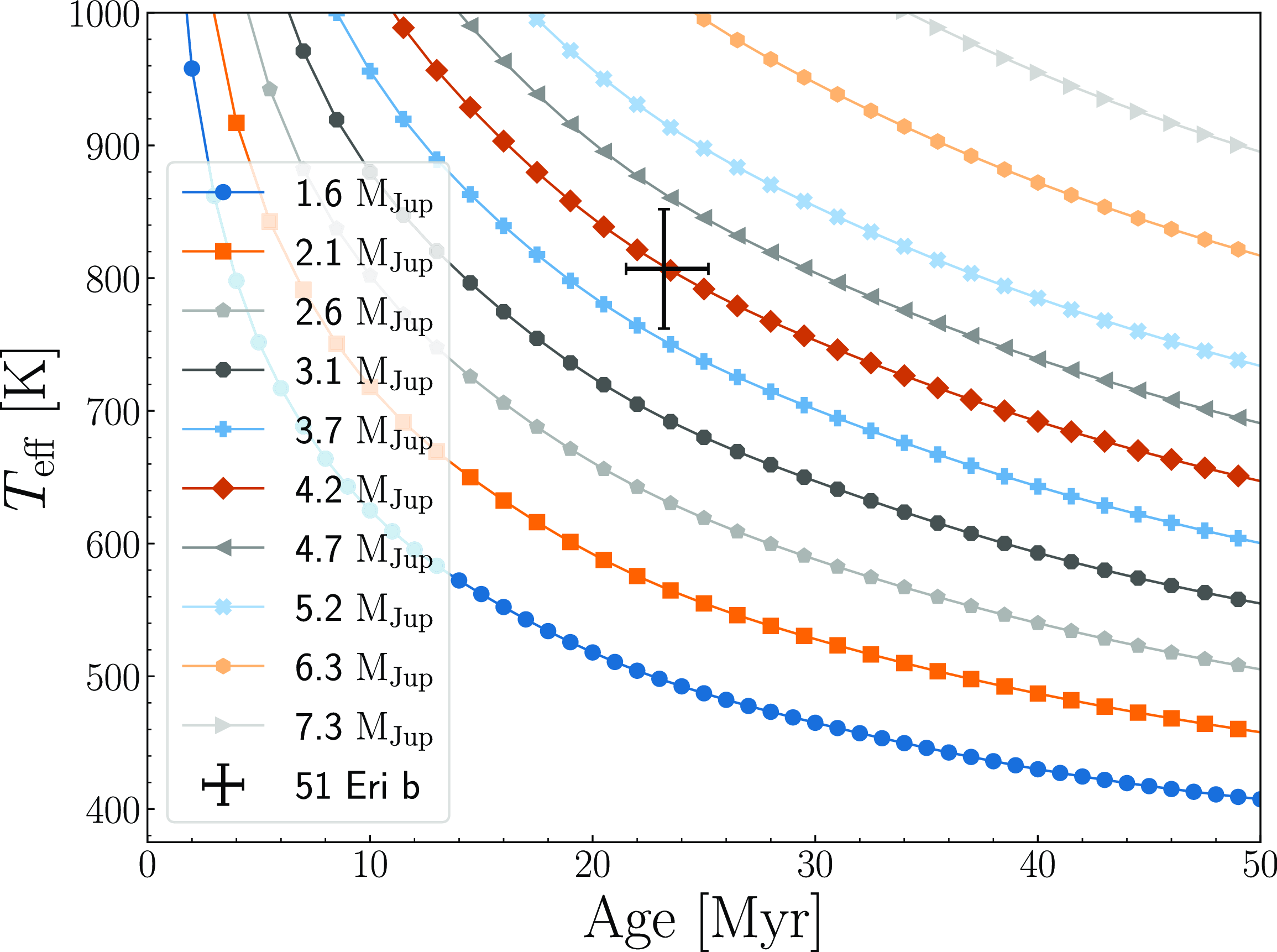
Figure 5. The planet iso-mass models from Marley et al. (Reference Marley2021). Iso-mass models were created using the The Sonora Bobcat model evolutionary tables that hold mass fixed. A one-dimensional interpolation was done to create a finer grid of points for each line. Then, a two-dimensional interpolation was done over $T_\mathrm{eff}$
and age to determine a planetary mass. For results, see Fig. 6 and Table 3.
$T_\mathrm{eff}$
and age to determine a planetary mass. For results, see Fig. 6 and Table 3.
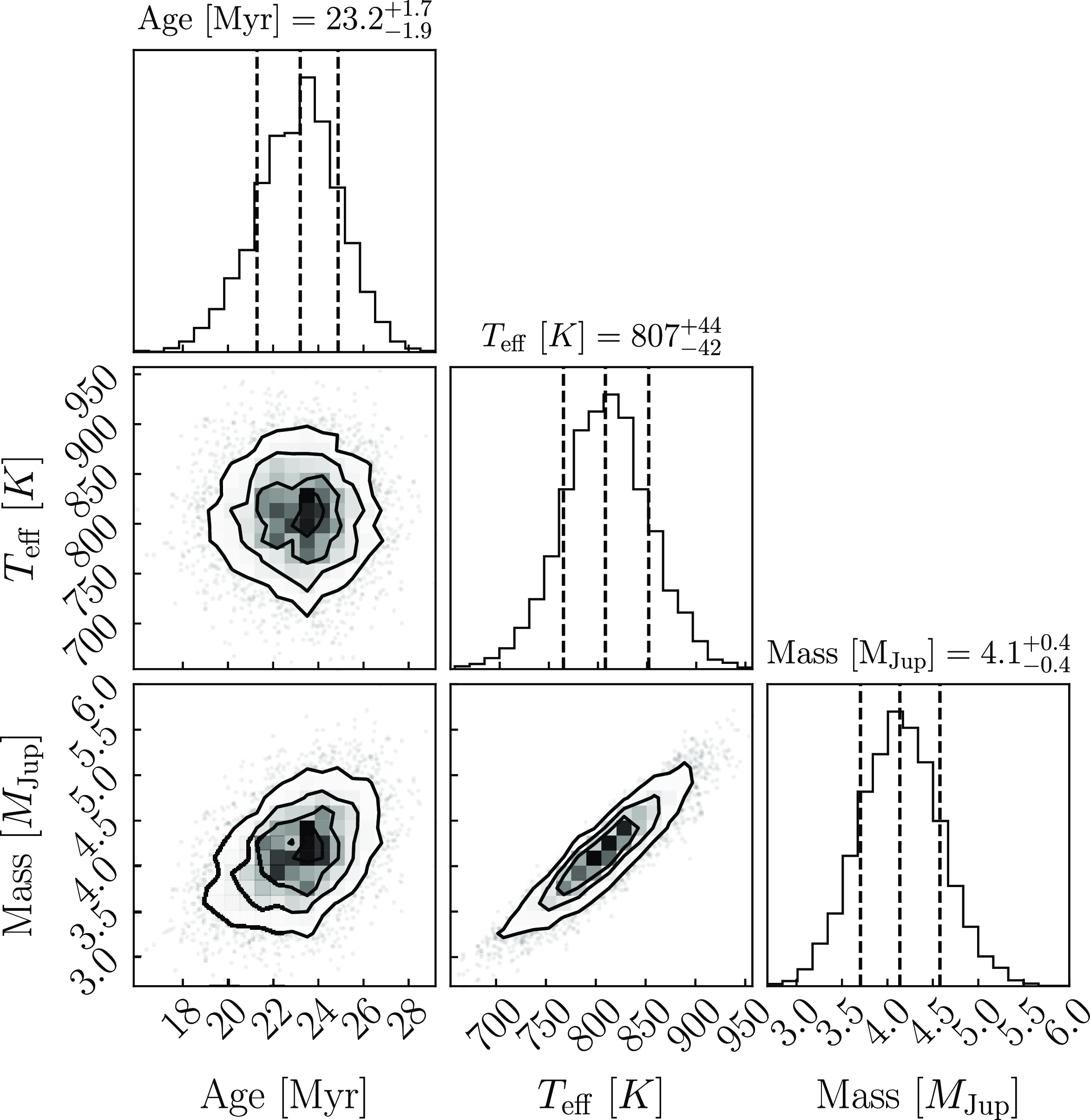
Figure 6. Corner plot for the Sonora Bobcat planet iso-mass model displaying the restuls of a Monte Carlo simulation of 5 000 iterations to estimate the mass of 51 Eri b. The dashed vertical lines indicate the quantiles for each histogram: $16 \%$
, 50%, and 84% from left to right. The left-most line corresponds to the lower bound uncertainty. The middle line corresponds to the accepted value. The right-most line corresponds to the upper-bound uncertainty. The final results of this simulation give a mass of
$16 \%$
, 50%, and 84% from left to right. The left-most line corresponds to the lower bound uncertainty. The middle line corresponds to the accepted value. The right-most line corresponds to the upper-bound uncertainty. The final results of this simulation give a mass of $4.1\pm 0.4$
M
$4.1\pm 0.4$
M $_\mathrm{Jup}$
. See Section 4.2 for details.
$_\mathrm{Jup}$
. See Section 4.2 for details.
5. Discussion
5.1. Stellar parameters
We measure a limb-darkened angular diameter for 51 Eridani of $\theta_\mathrm{LD} = 0.450 \pm 0.006$
mas (Section 4). We also measure an angular diameter of
$\theta_\mathrm{LD} = 0.450 \pm 0.006$
mas (Section 4). We also measure an angular diameter of $\theta_{LD} = 0.425 \pm 0.026$
mas using a LDC of
$\theta_{LD} = 0.425 \pm 0.026$
mas using a LDC of $\unicode{x03BC} = 0.2582$
from our CLASSIC data alone, which is consistent with the PAVO diameter within
$\unicode{x03BC} = 0.2582$
from our CLASSIC data alone, which is consistent with the PAVO diameter within $1\sigma$
. The PAVO measurement has a precision of less than 1%, compared to the CLASSIC measurement which has a precision of just over 6%. This is due to the greater spatial frequency coverage obtained with PAVO’s multiple wavelengths channels, as well as sampling further down the visibility curve to higher spatial frequencies. More coverage, especially at higher spatial frequencies, ensures that the visibility squared fit is more accurate. Simon and Schaefer (Reference Simon and Schaefer2011) measure an angular diameter of 51 Eridani also using CHARA’s CLASSIC beam combiner. Their measurements were taken in both H- and
$1\sigma$
. The PAVO measurement has a precision of less than 1%, compared to the CLASSIC measurement which has a precision of just over 6%. This is due to the greater spatial frequency coverage obtained with PAVO’s multiple wavelengths channels, as well as sampling further down the visibility curve to higher spatial frequencies. More coverage, especially at higher spatial frequencies, ensures that the visibility squared fit is more accurate. Simon and Schaefer (Reference Simon and Schaefer2011) measure an angular diameter of 51 Eridani also using CHARA’s CLASSIC beam combiner. Their measurements were taken in both H- and $K^{'}$
-band on the E1/W1 baseline (314 m). Simon and Schaefer (Reference Simon and Schaefer2011)’s angular diameter of
$K^{'}$
-band on the E1/W1 baseline (314 m). Simon and Schaefer (Reference Simon and Schaefer2011)’s angular diameter of $\theta_\mathrm{LD} = 0.518 \pm 0.009$
mas is over
$\theta_\mathrm{LD} = 0.518 \pm 0.009$
mas is over $7\sigma$
off from our PAVO angular diameter. We suspect that this disagreement is due to the observation strategy used by Simon and Schaefer (Reference Simon and Schaefer2011) who observed on a single baseline (E1/W1) and only used one calibrator in their analysis. This observation strategy is dangerously insensitive to verifying whether or not the single calibrator they used is good. In contrast, our measurements were taken using multiple calibrators over multiple nights (see Table 1). The angular diameter of 51 Eridani is near the resolution limit (
$7\sigma$
off from our PAVO angular diameter. We suspect that this disagreement is due to the observation strategy used by Simon and Schaefer (Reference Simon and Schaefer2011) who observed on a single baseline (E1/W1) and only used one calibrator in their analysis. This observation strategy is dangerously insensitive to verifying whether or not the single calibrator they used is good. In contrast, our measurements were taken using multiple calibrators over multiple nights (see Table 1). The angular diameter of 51 Eridani is near the resolution limit ( $\frac{\lambda}{2B}$
) of the CHARA Array on the longest baselines in the near-infrared. Analysis in the literature shows that interferometric measurements of under-resolved stars tend to systematically over-estimate their angular diameters (Casagrande et al. Reference Casagrande2014; White et al. Reference White2018; Tayar et al. Reference Tayar, Claytor, Huber and van Saders2022). However, our observations using CLASSIC data alone do not support this trend as they are in agreement within
$\frac{\lambda}{2B}$
) of the CHARA Array on the longest baselines in the near-infrared. Analysis in the literature shows that interferometric measurements of under-resolved stars tend to systematically over-estimate their angular diameters (Casagrande et al. Reference Casagrande2014; White et al. Reference White2018; Tayar et al. Reference Tayar, Claytor, Huber and van Saders2022). However, our observations using CLASSIC data alone do not support this trend as they are in agreement within $1\sigma$
of the PAVO observations.
$1\sigma$
of the PAVO observations.
Simon and Schaefer (Reference Simon and Schaefer2011) also performed an analysis to estimate the age and mass of 51 Eridani. This analysis used the PMS evolution models developed by Siess et al. (Reference Siess, Dufour and Forestini2000) and the Yonsei-Yale (Y2) models (Yi et al. Reference Yi, Kim and Demarque2003). Simon and Schaefer (Reference Simon and Schaefer2011) compared their absolute angular diameter (angular diameter scaled to a distance at 10 pc) with those predicted by both models and found an average age of $13\pm2$
Myr and a mass of
$13\pm2$
Myr and a mass of $1.75\pm0.05$
M
$1.75\pm0.05$
M $_{\odot}$
. Our age is almost twice that of Simon and Schaefer (Reference Simon and Schaefer2011), and our mass is
$_{\odot}$
. Our age is almost twice that of Simon and Schaefer (Reference Simon and Schaefer2011), and our mass is $4\sigma$
off of Simon and Schaefer (Reference Simon and Schaefer2011)’s. If we scale our angular measurement to a distance of 10 pc, it would fall closer to the older isochrones in Figure 3 in Simon and Schaefer (Reference Simon and Schaefer2011) for the same
$4\sigma$
off of Simon and Schaefer (Reference Simon and Schaefer2011)’s. If we scale our angular measurement to a distance of 10 pc, it would fall closer to the older isochrones in Figure 3 in Simon and Schaefer (Reference Simon and Schaefer2011) for the same $V-K$
, suggesting that the difference in angular diameter seems to be the main source of discrepancy. Additional errors are subject to arise in transforming the theoretical properties calculated by the models to observational quantities, such as magnitudes and colour indexes from colour tables. Comparing our directly measured
$V-K$
, suggesting that the difference in angular diameter seems to be the main source of discrepancy. Additional errors are subject to arise in transforming the theoretical properties calculated by the models to observational quantities, such as magnitudes and colour indexes from colour tables. Comparing our directly measured $T_\mathrm{eff}$
and luminosity to the model predictions ensures that any ambiguous errors that result from the colour tables will not affect our results.
$T_\mathrm{eff}$
and luminosity to the model predictions ensures that any ambiguous errors that result from the colour tables will not affect our results.
Simon and Schaefer (Reference Simon and Schaefer2011) also used a $V-K$
vs.
$V-K$
vs. $M_{K}$
diagram to estimate age and mass of 51 Eridani. The mass results were around
$M_{K}$
diagram to estimate age and mass of 51 Eridani. The mass results were around $0.2$
M
$0.2$
M $_{\odot}$
smaller than their initial analysis of comparing the model-predicted angular diameters and yielded older ages (around 5 Myr), creating a noted discrepancy between the two methods for age and mass. However, the
$_{\odot}$
smaller than their initial analysis of comparing the model-predicted angular diameters and yielded older ages (around 5 Myr), creating a noted discrepancy between the two methods for age and mass. However, the $V-K$
vs.
$V-K$
vs. $M_{K}$
result estimates align with our results.
$M_{K}$
result estimates align with our results.
The age we determine with the PARSEC model ( $23.2^{+1.7}_{-2.0}$
Myr) agrees with the age estimates found in the literature of both the star itself and that of the
$23.2^{+1.7}_{-2.0}$
Myr) agrees with the age estimates found in the literature of both the star itself and that of the $\beta PMG$
. These age estimates have been determined through a variety of methods from isochronal ages to lithium depletion methods. Mamajek and Bell (Reference Mamajek and Bell2014) conclude with an isochronal age of
$\beta PMG$
. These age estimates have been determined through a variety of methods from isochronal ages to lithium depletion methods. Mamajek and Bell (Reference Mamajek and Bell2014) conclude with an isochronal age of $22\pm 3$
Myr, where their value compares favourably to several lithium depletion boundary ages from Binks and Jeffries (Reference Binks and Jeffries2014) (
$22\pm 3$
Myr, where their value compares favourably to several lithium depletion boundary ages from Binks and Jeffries (Reference Binks and Jeffries2014) ( $21\pm4$
Myr) and Malo et al. (Reference Malo, Doyon, Feiden, Albert, Lafrenière, Artigau, Gagné and Riedel2014) (
$21\pm4$
Myr) and Malo et al. (Reference Malo, Doyon, Feiden, Albert, Lafrenière, Artigau, Gagné and Riedel2014) ( $26\pm3$
Myr).
$26\pm3$
Myr).
A more recent study on the $\beta PMG$
from Miret-Roig et al. (Reference Miret-Roig2020) concludes with an age estimate of
$\beta PMG$
from Miret-Roig et al. (Reference Miret-Roig2020) concludes with an age estimate of $18.5_{-2.4}^{+2.0}$
Myr through dynamical age trace-back methods using precise Gaia DR2 astrometry and ground-based radial velocities. Couture et al. (Reference Couture, Gagné and Doyon2023) developed a method to correct the trace-back age method that reduces the systemic errors from a combination of uncorrected gravitational red-shift and convective blue-shift absolute radial velocity measurements and the random errors from the parallax, proper motion, and additional radial velocity measurements. Their final resulting age is
$18.5_{-2.4}^{+2.0}$
Myr through dynamical age trace-back methods using precise Gaia DR2 astrometry and ground-based radial velocities. Couture et al. (Reference Couture, Gagné and Doyon2023) developed a method to correct the trace-back age method that reduces the systemic errors from a combination of uncorrected gravitational red-shift and convective blue-shift absolute radial velocity measurements and the random errors from the parallax, proper motion, and additional radial velocity measurements. Their final resulting age is $20.4 \pm 2.5$
Myr for the
$20.4 \pm 2.5$
Myr for the $\beta PMG$
. Our age estimate compares favourably to Couture et al. (Reference Couture, Gagné and Doyon2023)’s dynamical age estimates of the
$\beta PMG$
. Our age estimate compares favourably to Couture et al. (Reference Couture, Gagné and Doyon2023)’s dynamical age estimates of the $\beta PMG$
.
$\beta PMG$
.
5.2. A quick look at available TESS data
The Transiting Exoplanet Survey Satellite (TESS: Ricker et al. Reference Ricker2015) observed 51 Eridani in two sectors: Sector 5 and Sector 32. Sepulveda et al. (Reference Sepulveda, Huber, Zhang, Li, Liu and Bedding2022) investigated the variability seen in the TESS light curve data and concluded that 51 Eridani is a $\unicode{x03B3}$
-Dor pulsator. We downloaded the available 2-minute cadence data using lightkurve (Lightkurve Collaboration et al. 2018). The data were flattened and binned. From these data, we constructed a periodogram of the processed TESS data to search for significant exoplanet signals. We extracted significant frequencies and tested to see if a possible planet signal could be found. There were no significant possible planet signals. The light curves did show significant variability which does corroborate the findings of Sepulveda et al. (Reference Sepulveda, Huber, Zhang, Li, Liu and Bedding2022) in 51 Eridani being a
$\unicode{x03B3}$
-Dor pulsator. We downloaded the available 2-minute cadence data using lightkurve (Lightkurve Collaboration et al. 2018). The data were flattened and binned. From these data, we constructed a periodogram of the processed TESS data to search for significant exoplanet signals. We extracted significant frequencies and tested to see if a possible planet signal could be found. There were no significant possible planet signals. The light curves did show significant variability which does corroborate the findings of Sepulveda et al. (Reference Sepulveda, Huber, Zhang, Li, Liu and Bedding2022) in 51 Eridani being a $\unicode{x03B3}$
-Dor pulsator.
$\unicode{x03B3}$
-Dor pulsator.
5.3. Planetary parameters
We derive a mass for 51 Eri b to be $4.1\pm 0.4$
M
$4.1\pm 0.4$
M $_\mathrm{Jup}$
through the Sonora Bobcat evolutionary models (Section 4.2). Other studies have estimated the mass of 51 Eri b through a variety of methods, such as atmospheric modelling and evolutionary modelling. Several works present exploration of both methods, that is, using atmospheric modelling to obtain planetary parameters such as effective temperature, surface gravity, luminosity, and radius, and using these parameters along with an adopted age in evolutionary models to estimate a mass.
$_\mathrm{Jup}$
through the Sonora Bobcat evolutionary models (Section 4.2). Other studies have estimated the mass of 51 Eri b through a variety of methods, such as atmospheric modelling and evolutionary modelling. Several works present exploration of both methods, that is, using atmospheric modelling to obtain planetary parameters such as effective temperature, surface gravity, luminosity, and radius, and using these parameters along with an adopted age in evolutionary models to estimate a mass.
The initial discovery announcement of 51 Eri b (Macintosh et al. Reference Macintosh2015) performed atmospheric modelling to estimate the planet parameters, such as effective temperature and luminosity. Macintosh et al. (Reference Macintosh2015) used two separate models, a cloud-free and a partial cloudy model to obtain these parameters. The cloud-free model resulted in a $T_\mathrm{eff} = 750$
K and a log(
$T_\mathrm{eff} = 750$
K and a log( $L/\mathrm{L}_{\odot}) = -5.8$
. The partial cloudy model gave a
$L/\mathrm{L}_{\odot}) = -5.8$
. The partial cloudy model gave a $T_\mathrm{eff} = 700$
K and a log(
$T_\mathrm{eff} = 700$
K and a log( $L/\mathrm{L}_{\odot}) = -5.6$
. Macintosh et al. (Reference Macintosh2015) determined that the luminosity derived from the models does not change much with either model and used the luminosity along with age to estimate a mass based off of formation models. Given hot-start formation, the mass of 51 Eri b is
$L/\mathrm{L}_{\odot}) = -5.6$
. Macintosh et al. (Reference Macintosh2015) determined that the luminosity derived from the models does not change much with either model and used the luminosity along with age to estimate a mass based off of formation models. Given hot-start formation, the mass of 51 Eri b is $\sim 2$
M
$\sim 2$
M $_\mathrm{Jup}$
. With a cold-start formation, the mass falls in a range of 2–12 M
$_\mathrm{Jup}$
. With a cold-start formation, the mass falls in a range of 2–12 M $_\mathrm{Jup}$
. Our mass of
$_\mathrm{Jup}$
. Our mass of $4.1$
M
$4.1$
M $_\mathrm{Jup}$
is well within the cold-start formation range of ages but is over double that of the hot-start formation age.
$_\mathrm{Jup}$
is well within the cold-start formation range of ages but is over double that of the hot-start formation age.
Samland et al. (Reference Samland2017) presented the first spectro-photometric measurements in the Y- and K- bands of 51 Eri b using VLT/SPHERE. This study used atmospheric modelling using petitCODE – Cloudy to obtain planetary parameters. The resulting temperature, $T_\mathrm{eff} = 760 \pm 20$
K, radius of
$T_\mathrm{eff} = 760 \pm 20$
K, radius of $1.11^{+0.16}_{-0.14}$
R
$1.11^{+0.16}_{-0.14}$
R $_\mathrm{Jup}$
, and surface gravity of
$_\mathrm{Jup}$
, and surface gravity of $4.26 \pm 0.25$
(cgs-units) are used in a variety of methods to obtain mass estimates. Samland et al. (Reference Samland2017) used surface gravity and radius relations to get a mass of
$4.26 \pm 0.25$
(cgs-units) are used in a variety of methods to obtain mass estimates. Samland et al. (Reference Samland2017) used surface gravity and radius relations to get a mass of $9.1^{+4.9}_{-3.3}$
M
$9.1^{+4.9}_{-3.3}$
M $_\mathrm{Jup}$
which is Samland et al. (Reference Samland2017) also used radius and effective temperature relations to derive a luminosity and a planet formation model which relates luminosity and mass. The range in luminosity rules out the cold-start formation model and resulted in masses between 2.4 and 5 M
$_\mathrm{Jup}$
which is Samland et al. (Reference Samland2017) also used radius and effective temperature relations to derive a luminosity and a planet formation model which relates luminosity and mass. The range in luminosity rules out the cold-start formation model and resulted in masses between 2.4 and 5 M $_\mathrm{Jup}$
for the hot-start model and a larger spread of masses between 2 and 12 M
$_\mathrm{Jup}$
for the hot-start model and a larger spread of masses between 2 and 12 M $_\mathrm{Jup}$
for the warm-start model. Our mass also agrees with both mass ranges for the hot-start and warm-start models.
$_\mathrm{Jup}$
for the warm-start model. Our mass also agrees with both mass ranges for the hot-start and warm-start models.
Dupuy et al. (Reference Dupuy, Brandt and Brandt2022) performed a cross calibration of Hipparcos-GAIA astrometry and the orbit fitting code orvara. Their results provided orbital parameters as well as an upper limit on the mass of 51 Eri b of $< 11$
M
$< 11$
M $_\mathrm{Jup}$
. Through private communication, another run of the orvara fit was made using the new age and mass of 51 Eridani presented in this paper. The new upper limit
$_\mathrm{Jup}$
. Through private communication, another run of the orvara fit was made using the new age and mass of 51 Eridani presented in this paper. The new upper limit $2 \sigma$
constraint on the mass of 51 Eri b is 9.5 M
$2 \sigma$
constraint on the mass of 51 Eri b is 9.5 M $_\mathrm{Jup}$
. Our mass of
$_\mathrm{Jup}$
. Our mass of $4.1$
M
$4.1$
M $_\mathrm{Jup}$
clearly falls under this upper limit. Dupuy et al. (Reference Dupuy, Brandt and Brandt2022)’s result also indicated that the cold-start formation is ruled out given the derived initial entropy. They suggested that 51 Eri b formed similarly to other directly imaged planets which indicate either the warm or hot-start scenarios.
$_\mathrm{Jup}$
clearly falls under this upper limit. Dupuy et al. (Reference Dupuy, Brandt and Brandt2022)’s result also indicated that the cold-start formation is ruled out given the derived initial entropy. They suggested that 51 Eri b formed similarly to other directly imaged planets which indicate either the warm or hot-start scenarios.
The most recent study of 51 Eri b, done by Brown-Sevilla et al. (Reference Brown-Sevilla2023), revisited the work by Samland et al. (Reference Samland2017) and obtained new observations of 51 Eri b with VLT/SPHERE at a higher S/N than Samland et al. (Reference Samland2017)’s original data. Brown-Sevilla et al. (Reference Brown-Sevilla2023) used a new atmospheric retrieval code, petitRADTRANS, to update the $T_\mathrm{eff}$
and the resulting posterior distributions for the logg and planet radius to obtain a mass of
$T_\mathrm{eff}$
and the resulting posterior distributions for the logg and planet radius to obtain a mass of $3.9\pm 0.4$
M
$3.9\pm 0.4$
M $_\mathrm{Jup}$
. Sevilla et al. (Reference Brown-Sevilla2023) labelled this result as the nominal model. Brown-Sevilla et al. (Reference Brown-Sevilla2023) also performed an analysis using evolutionary models from Baraffe et al. (Reference Baraffe, Chabrier, Allard and Hauschildt2002) with two separate ages: 10 Myr (Lee et al. Reference Lee, Song and Murphy2022) and 20 Myr (Macintosh et al. Reference Macintosh2015), where they found masses of
$_\mathrm{Jup}$
. Sevilla et al. (Reference Brown-Sevilla2023) labelled this result as the nominal model. Brown-Sevilla et al. (Reference Brown-Sevilla2023) also performed an analysis using evolutionary models from Baraffe et al. (Reference Baraffe, Chabrier, Allard and Hauschildt2002) with two separate ages: 10 Myr (Lee et al. Reference Lee, Song and Murphy2022) and 20 Myr (Macintosh et al. Reference Macintosh2015), where they found masses of $2.4$
M
$2.4$
M $_\mathrm{Jup}$
and
$_\mathrm{Jup}$
and $2.6$
M
$2.6$
M $_\mathrm{Jup}$
, respectively. The mass presented in this work (
$_\mathrm{Jup}$
, respectively. The mass presented in this work ( $4.1\pm 0.4$
M
$4.1\pm 0.4$
M $_\mathrm{Jup}$
) agrees well with the nominal result obtained by Brown-Sevilla et al. (Reference Brown-Sevilla2023).
$_\mathrm{Jup}$
) agrees well with the nominal result obtained by Brown-Sevilla et al. (Reference Brown-Sevilla2023).
Our mass falls within the ranges of both the hot-start and the warm-start models as described by both Samland et al. (Reference Samland2017) and Brown-Sevilla et al. (Reference Brown-Sevilla2023). With our analysis, we can rule out a purely core accretion model as the main formation mechanism. Either scenario is likely, but future observations and analyses are needed to further test each model and develop a more conclusive argument.
6. Conclusion
In this work, we present interferometric observations of the directly imaged exoplanet host star 51 Eridani taken with both the PAVO and CLASSIC beam combiners at the CHARA Array. These observations resulted in a highly precise angular diameter measurement of 51 Eridani, $\theta_\mathrm{LD} = 0.450\pm0.006$
mas. From this angular diameter, we calculate the effective temperature,
$\theta_\mathrm{LD} = 0.450\pm0.006$
mas. From this angular diameter, we calculate the effective temperature, $T_\mathrm{eff} = 7\,422 \pm 58$
K, luminosity,
$T_\mathrm{eff} = 7\,422 \pm 58$
K, luminosity, $L_{\star} = 5.7\pm0.1$
L
$L_{\star} = 5.7\pm0.1$
L $_{\odot}$
, and linear radius,
$_{\odot}$
, and linear radius, $R_{\star} = 1.45\pm 0.02$
R
$R_{\star} = 1.45\pm 0.02$
R $_{\odot}$
. We use the PARSEC isochrones to derive an age of
$_{\odot}$
. We use the PARSEC isochrones to derive an age of $23.2^{+1.7}_{-2.0}$
Myr and mass of
$23.2^{+1.7}_{-2.0}$
Myr and mass of $1.550^{+0.006}_{-0.005}$
M
$1.550^{+0.006}_{-0.005}$
M $_{\odot}$
of 51 Eridani. For 51 Eri b, we estimate a mass of is
$_{\odot}$
of 51 Eridani. For 51 Eri b, we estimate a mass of is $4.1\pm 0.4$
M
$4.1\pm 0.4$
M $_\mathrm{Jup}$
using the Sonora Bobcat evolutionary models.
$_\mathrm{Jup}$
using the Sonora Bobcat evolutionary models.
Future analysis is encouraged using the JWST data taken in 2022 with NIRCAM and MIRI. Additional spectra can provide more constraints on planet composition, effective temperature, and luminosity when used with the atmospheric retrievals developed for JWST. Brown-Sevilla et al. (Reference Brown-Sevilla2023) suggested the use of the Mid-Infrared ELT Imager and Spectrograph (Quanz et al. Reference Quanz, Crossfield, Meyer, Schmalzl and Held2015) which will increase the wavelength coverage up to 13 $\mu$
m.
$\mu$
m.
Observations of other members of the $\beta PMG$
can help further the age constraints on these objects. In Table A1 in Alonso-Floriano et al. (Reference Alonso-Floriano, Caballero, Cortés-Contreras, Solano and Montes2015)’s paper, they list 185 members and candidate members of the
$\beta PMG$
can help further the age constraints on these objects. In Table A1 in Alonso-Floriano et al. (Reference Alonso-Floriano, Caballero, Cortés-Contreras, Solano and Montes2015)’s paper, they list 185 members and candidate members of the $\beta PMG$
. At least two F type stars are observable with PAVO at the CHARA Array and with future instruments being commissioned, such as the SPICA instrument (Mourard et al. Reference Mourard2017, Reference Mourard2022), the increased sensitivity will allow for more targets in this group to be observed. In addition, there are four stars that are accessible in the southern sky with VLTI that have angular diameters ranging between 0.46 and 0.75 mas (estimated using the surface brightness relationships in Adams et al. Reference Adams, Boyajian and von Braun2018). Two of these stars are observable with the current instrumentation available at VLTI. With the planned improvements to VLTI, such as adding the BIFROST (Kraus et al. Reference Kraus2022) instrument, the other two stars could be observable in the near future. Observing and characterising more stars within the
$\beta PMG$
. At least two F type stars are observable with PAVO at the CHARA Array and with future instruments being commissioned, such as the SPICA instrument (Mourard et al. Reference Mourard2017, Reference Mourard2022), the increased sensitivity will allow for more targets in this group to be observed. In addition, there are four stars that are accessible in the southern sky with VLTI that have angular diameters ranging between 0.46 and 0.75 mas (estimated using the surface brightness relationships in Adams et al. Reference Adams, Boyajian and von Braun2018). Two of these stars are observable with the current instrumentation available at VLTI. With the planned improvements to VLTI, such as adding the BIFROST (Kraus et al. Reference Kraus2022) instrument, the other two stars could be observable in the near future. Observing and characterising more stars within the $\beta$
PMG will help to estimate the age of the group and the individual stars within, giving us more insight on stellar evolution.
$\beta$
PMG will help to estimate the age of the group and the individual stars within, giving us more insight on stellar evolution.
Acknowledgements
This work is based upon observations obtained with the Georgia State University Center for High Angular Resolution Astronomy Array at Mount Wilson Observatory. The CHARA Array is supported by the National Science Foundation under Grant No. AST-1636624 and AST-2034336. Institutional support has been provided from the GSU College of Arts and Sciences and the GSU Office of the Vice President for Research and Economic Development.
CHARA telescope time was granted by NOIRLab through the Mid-Scale Innovations Program (MSIP). MSIP is funded by NSF.
CHARA Array time was granted through the NOIRLab community-access programme (NOIRLab Prop. ID: 2021A-0141; PI: T. Boyajian).
CHARA Array time was granted through the NOIRLab community-access program (NOIRLab Prop. ID: 2021A-0247; PI: T. Ellis).
We thank Dr. Gururaj A. Wagle for his assistance in understanding interpolation and Henry Ngo for the extremely helpful suggestions in debugging interpolation code. We also thank Nageeb Zaman and Dr. Jonas Klüter for their assistance in developing an asymmetrical normal distribution for Monte Carlo simulations used in this work.
This research has made use of the VizieR catalogue access tool, CDS, Strasbourg, France (DOI : 10.26093/cds/vizier). The original description of the VizieR service was published in 2000, A&AS 143, 23 (Ochsenbein et al. Reference Ochsenbein, Bauer and Marcout2000).
This research has made use of the Jean-Marie Mariotti Center JSDC catalogue.Footnote c
This research has made use of the Jean-Marie Mariotti Center Aspro Footnote d service.
This paper includes data collected by the TESS mission. Funding for the TESS mission is provided by the NASA’s Science Mission Directorate.
This research made use of Lightkurve, a Python package for Kepler and TESS data analysis (Lightkurve Collaboration et al. 2018).
Data availability statement
All interferometric data are available in the CHARA archive.Footnote e The TESS observations are available in the Barbara A. Mikulski Archive for Space Telescopes (MAST) archive.
Financial support
A.E. and T.S.B. acknowledge support by the National Support Foundation under Grant No. AST-2205914.
Competing interests
None.


