


1. Introduction
The Milky Way galaxy is a complex and dynamic system that has undergone a long and rich history of formation and evolution. One of the main goals of galactic archaeology is to reconstruct this history by studying the properties of its stellar populations, especially the oldest and most pristine ones. Stars carry valuable information about their birth environments’ physical and chemical conditions. By measuring their photospheric elemental abundances, we can infer the nucleosynthesis processes that enriched the interstellar medium (ISM) at the time of their birth, the star formation rates (SFR), the mixing and transport mechanisms, and the merger events that shaped the Galaxy. However, it remains a challenge to identify the ancient in situ stars that formed in the pre-disk phase of our galaxy. The elemental abundances of these stars are expected to reveal the initial conditions of our galaxy that set the stage for disk formation.
Stellar photospheric elemental abundances are one of the most powerful tools for galactic archaeology because they are expected to remain the same over the lifetime of the stars as demonstrated by the chemical homogeneity of open clusters (De Silva et al. Reference De Silva, Sneden, Paulson, Asplund, Bland-Hawthorn, Bessell and Freeman2006, Reference De Silva, Freeman, Asplund, Bland-Hawthorn, Bessell and Collet2007; Reddy, Giridhar, & Lambert Reference Reddy, Giridhar and Lambert2012; Ting et al. Reference Ting, Freeman, Kobayashi, De Silva and Bland-Hawthorn2012; Bovy Reference Bovy2016; Poovelil et al. Reference Poovelil2020; Cheng, Price-Jones, & Bovy Reference Cheng, Price-Jones and Bovy2021). Different elements are produced by various sources, such as massive stars, Type Ia supernovae (SNe Ia), asymptotic giant branch (AGB) stars, or neutron star mergers, with different delay timescales and efficiencies (Tinsley Reference Tinsley1980; Nomoto, Kobayashi, & Tominaga Reference Nomoto, Kobayashi and Tominaga2013; Kobayashi et al. Reference Kobayashi, Umeda, Nomoto, Tomi-naga and Ohkubo2006; Maoz & Graur 2012; Kobayashi, Karakas, & Lugaro Reference Kobayashi, Karakas and Lugaro2020). Certain elements, such as oxygen, neon, magnesium, silicon, sulphur, argon, calcium, and titanium, can be produced at early times in core-collapse events at relatively constant rates with iron. Stars with high [ $\alpha$
/Fe] tend to form early when
$\alpha$
/Fe] tend to form early when $\alpha$
-producing core-collapse supernovae (CCSN) dominate nucleosynthesis (Limongi & Chieffi Reference Limongi and Chieffi2003, Reference Limongi, Chieffi, Kubono, Aoki, Kajino, Motobayashi and Nomoto2006; Nomoto et al. Reference Nomoto, Tominaga, Umeda, Kobayashi and Maeda2006). As time passes and Type Ia supernovae ‘turn on’ through different progenitor scenarios (Hillebrandt et al. Reference Hillebrandt, Kromer, Röpke and Ruiter2013; Ruiter Reference Ruiter, Barstow, Kleinman, Provencal and Ferrario2020), the [
$\alpha$
-producing core-collapse supernovae (CCSN) dominate nucleosynthesis (Limongi & Chieffi Reference Limongi and Chieffi2003, Reference Limongi, Chieffi, Kubono, Aoki, Kajino, Motobayashi and Nomoto2006; Nomoto et al. Reference Nomoto, Tominaga, Umeda, Kobayashi and Maeda2006). As time passes and Type Ia supernovae ‘turn on’ through different progenitor scenarios (Hillebrandt et al. Reference Hillebrandt, Kromer, Röpke and Ruiter2013; Ruiter Reference Ruiter, Barstow, Kleinman, Provencal and Ferrario2020), the [ $\alpha$
/Fe] ratio drops as the rate of iron production accelerates. This evolution of [
$\alpha$
/Fe] ratio drops as the rate of iron production accelerates. This evolution of [ $\alpha$
/Fe] over time has been quantified in large spectroscopic surveys, thanks to innovative methods of measuring stellar ages (Sharma et al. Reference Sharma2022; Ratcliffe et al. Reference Ratcliffe2023). The relative abundances of different elements can thus reflect the relative contributions of these separate sources as well as the time delay between their production and their incorporation into new generations of stars. Tracing the elemental abundance ratios over time provides direct and robust constraints on the chemical evolution of the galaxy.
$\alpha$
/Fe] over time has been quantified in large spectroscopic surveys, thanks to innovative methods of measuring stellar ages (Sharma et al. Reference Sharma2022; Ratcliffe et al. Reference Ratcliffe2023). The relative abundances of different elements can thus reflect the relative contributions of these separate sources as well as the time delay between their production and their incorporation into new generations of stars. Tracing the elemental abundance ratios over time provides direct and robust constraints on the chemical evolution of the galaxy.
Massive disk galaxies like the Milky Way are expected to have an ancient, metal-poor, and centrally concentrated stellar population, reflecting the star formation and enrichment in the most massive progenitor components at high redshift. Hopkins et al. (Reference Hopkins2023) showed that a centrally concentrated mass profile is necessary for disk formation with Feedback In Realistic Environments (FIRE) simulation. Metal-poor stars are known to reside in the inner few kiloparsecs of the Milky Way (García et al. Reference García2013; Arentsen et al. Reference Arentsen2020a,b), but the current data does not provide a comprehensive picture of this metal-poor ‘heart’ of the Milky Way. However, recent observations taking advantage of the XP spectra from Gaia DR3 have revealed an extensive, ancient, and metal-poor population of stars in the inner galaxy, representing a significant stellar mass (Rix et al. Reference Rix2022). The early phases of the Milky Way’s star formation and enrichment are reflected in the distribution of old and metal-poor stars, which can be a mix of those that formed within the main in situ over-densities of the proto-Galaxy and those that formed in distinct satellite galaxies that later merged with the main body (Horta et al. Reference Horta2021b). The distinction between in situ formation and accretion can be seen in the abundance patterns of the stars, although at very early epochs, the distinction may become blurry due to the rapid coalescence of comparable mass pieces in major mergers. Recently, this has been verified by Horta et al. (Reference Horta2023a) which found most prototypes of the Milky Way in the FIRE-2 cosmological zoom-in simulations formed in group environments rather than in isolation.
Recent observational evidence has shed light on the chemical evolution of the transition period when the disk started forming in the Milky Way. Belokurov & Kravtsov (Reference Belokurov and Kravtsov2022) identified a metal-poor component in the Milky Way called Aurora from the APOGEE survey. This component is kinematically hot, with an approximately isotropic velocity ellipsoid and a modest net rotation. They revealed that the in situ stars in Aurora exhibit a large scatter in elemental abundance ratios, and the median tangential velocity of the in situ stars increases sharply with increasing metallicity when [Fe/H] is between $-1.3$
and
$-1.3$
and $-0.9$
. The chemical scatter suddenly drops after this period, signalling the formation of the disk in about one to two Gyr. They proposed that these observed trends in the Milky Way reflect generic processes during the early evolution of progenitors of Milky-Way-sized galaxies, including a period of chaotic pre-disk evolution and subsequent rapid disk settlement. Interestingly, many of the most metal poor in situ stars preceding the disk populations in their sample have lower [Mg/Fe] than the traditional high [Mg/Fe] associated with old stars in the Galaxy (see their figures 6 and 7).
$-0.9$
. The chemical scatter suddenly drops after this period, signalling the formation of the disk in about one to two Gyr. They proposed that these observed trends in the Milky Way reflect generic processes during the early evolution of progenitors of Milky-Way-sized galaxies, including a period of chaotic pre-disk evolution and subsequent rapid disk settlement. Interestingly, many of the most metal poor in situ stars preceding the disk populations in their sample have lower [Mg/Fe] than the traditional high [Mg/Fe] associated with old stars in the Galaxy (see their figures 6 and 7).
Conroy et al. (Reference Conroy2022) extended the search for in situ halo stars as metal-poor as [Fe/H] = –2.5 in the H3 survey (Conroy et al. Reference Conroy2019) and revealed that [ $\alpha$
/Fe] gradually declined at low metallicity and rose around [Fe/H]
$\alpha$
/Fe] gradually declined at low metallicity and rose around [Fe/H] $= -1.3$
instead of declining monotonically (see their figure 1). Rix et al. (Reference Rix2022) derived reliable metallicity estimates for about two million bright stars from the XP spectra of Gaia DR3, including 18 000 stars with
$= -1.3$
instead of declining monotonically (see their figure 1). Rix et al. (Reference Rix2022) derived reliable metallicity estimates for about two million bright stars from the XP spectra of Gaia DR3, including 18 000 stars with $-2.7 <$
[M/H]
$-2.7 <$
[M/H] $< -1.5$
. This massive sample allowed them to present the most comprehensive collection of metal-poor in situ stars in the Milky Way. They showed that the observed [
$< -1.5$
. This massive sample allowed them to present the most comprehensive collection of metal-poor in situ stars in the Milky Way. They showed that the observed [ $\alpha$
/Fe]-rise is robust even for stars on near-circular orbits in their sample supplemented by [Mg/Fe] from APOGEE (their figure 7). Again, the unexpected [
$\alpha$
/Fe]-rise is robust even for stars on near-circular orbits in their sample supplemented by [Mg/Fe] from APOGEE (their figure 7). Again, the unexpected [ $\alpha$
/Fe]-rise has also been found among metal-poor in situ globular clusters (Belokurov & Kravtsov Reference Belokurov and Kravtsov2023). Despite using samples from different surveys and selection methods, all of their works showed an [
$\alpha$
/Fe]-rise has also been found among metal-poor in situ globular clusters (Belokurov & Kravtsov Reference Belokurov and Kravtsov2023). Despite using samples from different surveys and selection methods, all of their works showed an [ $\alpha$
/Fe]-rise between [Fe/H] = -1.3 and -1 among preferentially in situ stars.
$\alpha$
/Fe]-rise between [Fe/H] = -1.3 and -1 among preferentially in situ stars.
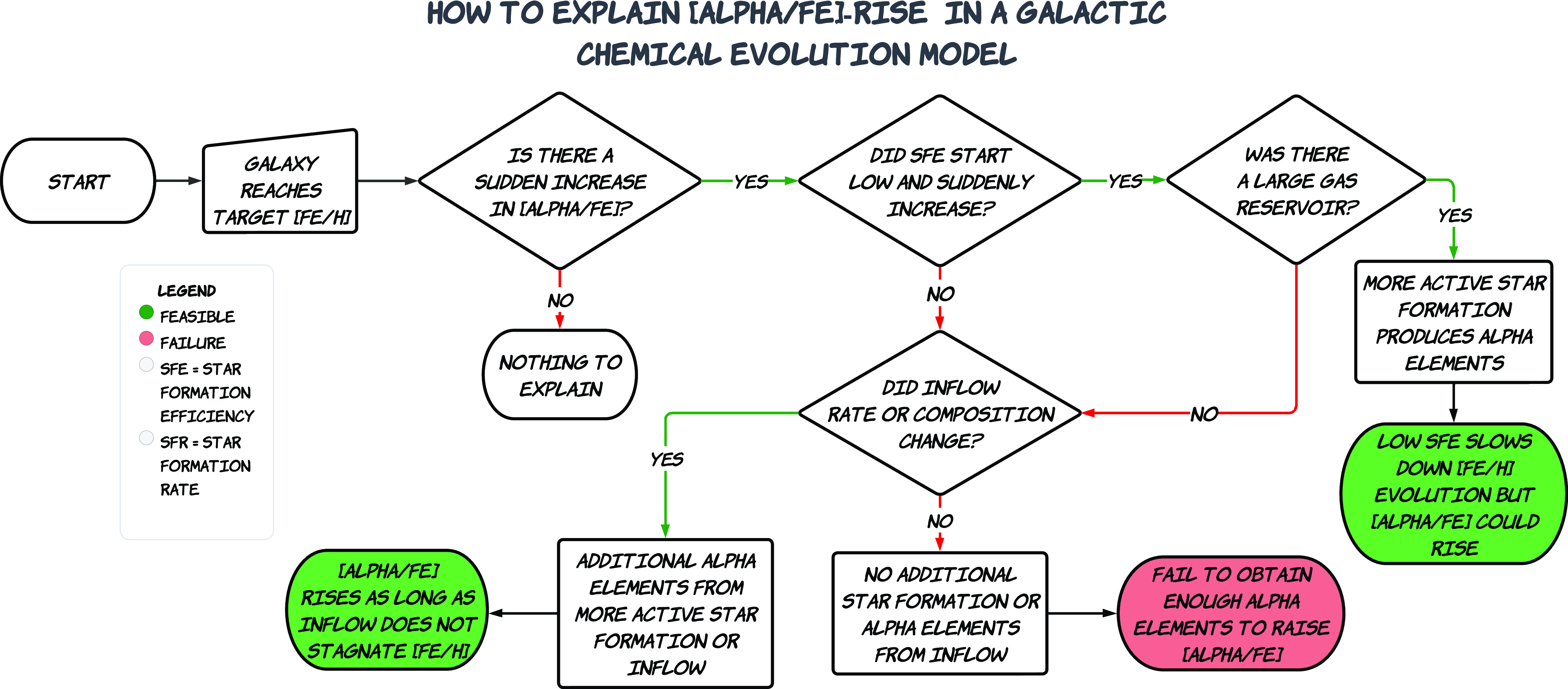
Figure 1. Flowchart illustrating scenarios of early Milky Way chemical evolution. The scenario capable of producing an [ $\alpha$
/Fe]-rise is highlighted in green and the rest in red. In summary, the additional star formation required to raise [
$\alpha$
/Fe]-rise is highlighted in green and the rest in red. In summary, the additional star formation required to raise [ $\alpha$
/Fe] can be achieved by increasing the SFE, inflow rate, or both. However, increasing the SFE is ineffective if no gas sustains star formation. If the gas already exists as a massive gas reservoir before the parameter change, it is difficult to change the abundance in the model. The inflow should join the model after the parameter change.
$\alpha$
/Fe] can be achieved by increasing the SFE, inflow rate, or both. However, increasing the SFE is ineffective if no gas sustains star formation. If the gas already exists as a massive gas reservoir before the parameter change, it is difficult to change the abundance in the model. The inflow should join the model after the parameter change.
The decline in [ $\alpha$
/Fe] is expected in all galaxies in time as remnants from intermediate-mass stars (
$\alpha$
/Fe] is expected in all galaxies in time as remnants from intermediate-mass stars ( $\sim$
3–8
$\sim$
3–8 $\mathrm{M}_\odot$
) explode as SNe Ia and release iron-peak elements unless an increasing amount of massive stars are continually evolving as CCSNe and releasing
$\mathrm{M}_\odot$
) explode as SNe Ia and release iron-peak elements unless an increasing amount of massive stars are continually evolving as CCSNe and releasing $\alpha$
elements to balance [
$\alpha$
elements to balance [ $\alpha$
/Fe] due to the rarity of massive stars. However, it is surprising to witness an increase in [
$\alpha$
/Fe] due to the rarity of massive stars. However, it is surprising to witness an increase in [ $\alpha$
/Fe] after it has started to drop as shown in recent observations. This signals the introduction of a considerable amount of
$\alpha$
/Fe] after it has started to drop as shown in recent observations. This signals the introduction of a considerable amount of $\alpha$
elements into our Galaxy after SNe Ia have made an impact on the composition of the ISM. The ‘simmering’ phase scenario was proposed by Conroy et al. (Reference Conroy2022) to explain the rise in [
$\alpha$
elements into our Galaxy after SNe Ia have made an impact on the composition of the ISM. The ‘simmering’ phase scenario was proposed by Conroy et al. (Reference Conroy2022) to explain the rise in [ $\alpha$
/Fe]. They fixed the inflow rate constant and adopted a low SFE as [
$\alpha$
/Fe]. They fixed the inflow rate constant and adopted a low SFE as [ $\alpha$
/Fe] naturally declined due to the onset of SNe Ia to avoid forming too many metal-poor stars. As [
$\alpha$
/Fe] naturally declined due to the onset of SNe Ia to avoid forming too many metal-poor stars. As [ $\alpha$
/Fe] reached the lowest point, they increased the SFE in the model by twenty-five times. Many massive stars form and evolve as a result and CCSNe dominate the nucleosynthesis process causing [
$\alpha$
/Fe] reached the lowest point, they increased the SFE in the model by twenty-five times. Many massive stars form and evolve as a result and CCSNe dominate the nucleosynthesis process causing [ $\alpha$
/Fe] to rise. However, a low SFE could hinder the evolution of [Fe/H] in the proto Milky Way and a twenty-five-fold increase in the SFE is rare in isolated galaxies and requires specific galaxy interactions and mergers (Di Matteo et al. Reference Di Matteo, Bournaud, Martig, Combes, Melchior and Semelin2008).
$\alpha$
/Fe] to rise. However, a low SFE could hinder the evolution of [Fe/H] in the proto Milky Way and a twenty-five-fold increase in the SFE is rare in isolated galaxies and requires specific galaxy interactions and mergers (Di Matteo et al. Reference Di Matteo, Bournaud, Martig, Combes, Melchior and Semelin2008).
Another feasible scenario is that the [ $\alpha$
/Fe]-rise was a symptom of fluctuations in the inflow history. The gas reservoir was kept small as [Fe/H] rose and [
$\alpha$
/Fe]-rise was a symptom of fluctuations in the inflow history. The gas reservoir was kept small as [Fe/H] rose and [ $\alpha$
/Fe] declined and a large amount of gas joined through inflow. The additional
$\alpha$
/Fe] declined and a large amount of gas joined through inflow. The additional $\alpha$
elements could be brought in through high-[
$\alpha$
elements could be brought in through high-[ $\alpha$
/Fe] gas or from the enhanced star formation due to more gas available. Under this scenario, the SFE could remain high throughout the entire proto-Galaxy phase to facilitate the rapid chemical evolution during the early Milky Way. Fuelling star formation with additional gas could also sustain star formation which lasts billions of years in the Milky Way. However, there is a large uncertainty in the composition of inflow gas. A substantial amount of metal-poor gas could potentially stifle the evolution of [Fe/H] for an extended period. A flowchart in Fig. 1 illustrates the reasoning that leads to these two feasible scenarios, which we will revisit after presenting our results.
$\alpha$
/Fe] gas or from the enhanced star formation due to more gas available. Under this scenario, the SFE could remain high throughout the entire proto-Galaxy phase to facilitate the rapid chemical evolution during the early Milky Way. Fuelling star formation with additional gas could also sustain star formation which lasts billions of years in the Milky Way. However, there is a large uncertainty in the composition of inflow gas. A substantial amount of metal-poor gas could potentially stifle the evolution of [Fe/H] for an extended period. A flowchart in Fig. 1 illustrates the reasoning that leads to these two feasible scenarios, which we will revisit after presenting our results.
This work aims to investigate the cause behind the [ $\alpha$
/Fe]-rise comprehensively with a galactic chemical evolution (GCE) model, specifically how much of a role gas inflow can play. GCE models are a computationally efficient approach to studying the evolution of galaxies, particularly their elemental abundances. They use parametric empirical laws to trace the evolution of abundances without directly modelling star formation and gas accretion history as performed in cosmological simulations. They have managed to replicate the age-metallicity and age-[
$\alpha$
/Fe]-rise comprehensively with a galactic chemical evolution (GCE) model, specifically how much of a role gas inflow can play. GCE models are a computationally efficient approach to studying the evolution of galaxies, particularly their elemental abundances. They use parametric empirical laws to trace the evolution of abundances without directly modelling star formation and gas accretion history as performed in cosmological simulations. They have managed to replicate the age-metallicity and age-[ $\alpha$
/Fe] relationship, the stellar density variation in the [Fe/H]-[
$\alpha$
/Fe] relationship, the stellar density variation in the [Fe/H]-[ $\alpha$
/Fe]-plane as a function of positions in the Milky Way (Minchev et al. Reference Minchev2018; Haywood et al. Reference Haywood, Snaith, Lehnert, Di Matteo and Khoperskov2019; Sharma, Hayden, & Bland-Hawthorn Reference Sharma, Hayden and Bland-Hawthorn2021; Johnson et al. Reference Johnson2021; Chen et al. Reference Chen, Hayden, Sharma, Bland-Hawthorn, Kobayashi and Karakas2023). The remainder of this paper is organized as follows: Section 2 gives an introduction to GCE models and briefly describes the ingredients in our model. Section 3 shows the parameter distribution for the models that satisfy part or all of the descriptions of the observed [
$\alpha$
/Fe]-plane as a function of positions in the Milky Way (Minchev et al. Reference Minchev2018; Haywood et al. Reference Haywood, Snaith, Lehnert, Di Matteo and Khoperskov2019; Sharma, Hayden, & Bland-Hawthorn Reference Sharma, Hayden and Bland-Hawthorn2021; Johnson et al. Reference Johnson2021; Chen et al. Reference Chen, Hayden, Sharma, Bland-Hawthorn, Kobayashi and Karakas2023). The remainder of this paper is organized as follows: Section 2 gives an introduction to GCE models and briefly describes the ingredients in our model. Section 3 shows the parameter distribution for the models that satisfy part or all of the descriptions of the observed [ $\alpha$
/Fe] behavior. Section 4 discusses the implications of our results in light of recent work on the early Milky Way. Section 5 provides a summary of our results.
$\alpha$
/Fe] behavior. Section 4 discusses the implications of our results in light of recent work on the early Milky Way. Section 5 provides a summary of our results.
2. Model
GCE models utilize a set of parameters guided by empirical physical laws to simulate the chemical evolutionary trajectory of galaxies. The synthesis of new elements within stars and the subsequent release and recycling of gas consisting of these newly produced elements into star formation are critical components of these models. Further mechanisms such as accretion/inflow (introducing fresh gas into the model) and outflow (removing existing ISM) can directly or indirectly shape the chemical evolution depicted by these models. The computational time required to run these models is a fraction of what it takes to trace chemistry in cosmological simulations. Therefore, they allow us to quickly sample an extensive range of parameters to examine the impact of various mechanisms or events on the chemistry of galaxies.
The model utilized in this work was originally developed by Andrews et al. (Reference Andrews, Weinberg, Schönrich and Johnson2017) named flexCE. We kept most of the original design, except for a few ingredients. The model has many features that make it ideal for exploring the physical conditions of galaxies through elemental abundances. First, it has a multi-phase ISM composed of a cold and warm component, thus relaxing the assumption of instantaneous recycling in most GCE models. The newly synthesized nucleosynthesis yields are not immediately returned to the cold ISM for the next round of star formation. Instead, they are stored in the warm ISM which cooled gradually over time. Second, it has a physical implementation of star formation and evolution. The amount of star formation activity in any given step is determined by the amount of cold ISM at the time and the stars are represented in stellar mass bins with lifetimes. The SFH in the model is regulated by the mechanisms and thus self-consistent. The original stellar lifetimes only depended on the progenitor mass through an analytic function. Instead, we sourced stellar lifetimes from PARSEC-1.2S isochrones of various progenitor masses and metallicities (Bressan et al. Reference Bressan, Marigo, Girardi, Salasnich, Cero, Rubele and Nanni2012). The tracking of stellar lifetimes is important for studying the nucleosynthesis inside low-mass stars, including the production of white dwarfs (WD) and the occurrence of SNe Ia.
Third, it uses a complete suite of nucleosynthesis tables from major channels. We use the tables from Nomoto, Kobayashi, & Tominaga (Reference Nomoto, Kobayashi and Tominaga2013) which covers SNe Ia, CCSNe, and AGB stars from 0.9 to 40 $\mathrm{M}_\odot$
. This allows us to trace up to 32 elements in the model. Lastly, the model has a large selection of free parameters that allow us to fine-tune the strengths of various mechanisms. We can prescribe a function that controls the inflow of fresh gas over time and adjust the mass-loading factor regulating the outflow from star formation and supernovae. The original model assigned the inflowing gas to the cold ISM when it joins the model, but we switched it to the warm ISM. The fresh gas mixes with the existing warm ISM before it cools to fuel star formation. The cooling of the inflowing gas is governed by the same cooling timescale for the existing warm ISM. This change improves the smoothness of chemical evolutionary tracks when a large amount of gas with a different composition joins the model. Section 2.1 offers a brief description of the model for readers not familiar with the original version. More details can be found in Chen et al. (Reference Chen, Hayden, Sharma, Bland-Hawthorn, Kobayashi and Karakas2023) where a multi-zone version of this model replicated the variation of the [Fe/H]-[
$\mathrm{M}_\odot$
. This allows us to trace up to 32 elements in the model. Lastly, the model has a large selection of free parameters that allow us to fine-tune the strengths of various mechanisms. We can prescribe a function that controls the inflow of fresh gas over time and adjust the mass-loading factor regulating the outflow from star formation and supernovae. The original model assigned the inflowing gas to the cold ISM when it joins the model, but we switched it to the warm ISM. The fresh gas mixes with the existing warm ISM before it cools to fuel star formation. The cooling of the inflowing gas is governed by the same cooling timescale for the existing warm ISM. This change improves the smoothness of chemical evolutionary tracks when a large amount of gas with a different composition joins the model. Section 2.1 offers a brief description of the model for readers not familiar with the original version. More details can be found in Chen et al. (Reference Chen, Hayden, Sharma, Bland-Hawthorn, Kobayashi and Karakas2023) where a multi-zone version of this model replicated the variation of the [Fe/H]-[ $\alpha$
/Fe] density distribution in various locations of the cross-section plane of the Milky Way.
$\alpha$
/Fe] density distribution in various locations of the cross-section plane of the Milky Way.
2.1. Setting up our GCE model
To investigate the [ $\alpha$
/Fe] behaviour at the outset of the Milky Way’s evolution, our model is set to run for only two Gyr. The maximum time is chosen to accommodate a subsequent high-[
$\alpha$
/Fe] behaviour at the outset of the Milky Way’s evolution, our model is set to run for only two Gyr. The maximum time is chosen to accommodate a subsequent high-[ $\alpha$
/Fe] disk population that could potentially be as ancient as twelve billion years old according to Xiang & Rix (Reference Xiang and Rix2022) who found that the disk could have started forming as early as 800 Myr after the Big Bang and most metal-poor thick disk stars formed between ten and twelve Gyr ago. We divided the time frame into two phases, the first one lasting one Gyr allowing [
$\alpha$
/Fe] disk population that could potentially be as ancient as twelve billion years old according to Xiang & Rix (Reference Xiang and Rix2022) who found that the disk could have started forming as early as 800 Myr after the Big Bang and most metal-poor thick disk stars formed between ten and twelve Gyr ago. We divided the time frame into two phases, the first one lasting one Gyr allowing [ $\alpha$
/Fe] to decline and the second one lasting another one Gyr as [
$\alpha$
/Fe] to decline and the second one lasting another one Gyr as [ $\alpha$
/Fe] rises. Each time step corresponds to
$\alpha$
/Fe] rises. Each time step corresponds to $dt = 30$
Myr, reflecting the lifespan of the longest-living progenitors of CCSNe. Given that the proto-Galaxy was likely considerably smaller than the current Milky Way, our circular box is assigned a radius of
$dt = 30$
Myr, reflecting the lifespan of the longest-living progenitors of CCSNe. Given that the proto-Galaxy was likely considerably smaller than the current Milky Way, our circular box is assigned a radius of $R=1$
kpc. The yield tables from Nomoto, Kobayashi, & Tominaga (Reference Nomoto, Kobayashi and Tominaga2013) are interpolated across the available metallicity values to accommodate any given metallicity.
$R=1$
kpc. The yield tables from Nomoto, Kobayashi, & Tominaga (Reference Nomoto, Kobayashi and Tominaga2013) are interpolated across the available metallicity values to accommodate any given metallicity.
We now initialize the components in our GCE model that will house the chemical elements: stars, cold ISM, and warm ISM. The stars are represented by stellar bins ranging from 0.5 to 40 $\mathrm{M}_\odot$
, following the initial mass function (IMF) defined below:
$\mathrm{M}_\odot$
, following the initial mass function (IMF) defined below:
 \begin{equation}\xi(m) \propto m^{-2.3}\end{equation}
Although stars less massive than 0.9 $\mathrm{M}_\odot$
are formed in our model, they do not participate in nucleosynthesis. This is also true if we extend the minimum stellar mass below 0.5
$\mathrm{M}_\odot$
are formed in our model, they do not participate in nucleosynthesis. This is also true if we extend the minimum stellar mass below 0.5 $\mathrm{M}_\odot$
. Including additional low-mass stars would make nucleosynthesis less efficient for the same amount of stellar mass formed. Stars more massive than 9
$\mathrm{M}_\odot$
. Including additional low-mass stars would make nucleosynthesis less efficient for the same amount of stellar mass formed. Stars more massive than 9 $\mathrm{M}_\odot$
only survive for less than 30 Myr and will end their lifetime within a single time step. New stellar bins are created to contain the mass during star formation at each step, and we monitor the remaining mass over time. In addition to mass, we also log the gas composition encapsulated within the stars at the moment of formation. This chemical composition is updated when a stellar bin expires according to the interpolated yield tables. When a star with a mass between 3 and 8
$\mathrm{M}_\odot$
only survive for less than 30 Myr and will end their lifetime within a single time step. New stellar bins are created to contain the mass during star formation at each step, and we monitor the remaining mass over time. In addition to mass, we also log the gas composition encapsulated within the stars at the moment of formation. This chemical composition is updated when a stellar bin expires according to the interpolated yield tables. When a star with a mass between 3 and 8 $\mathrm{M}_\odot$
dies, we reference its remnant mass in the yield tables and add it to a WD reservoir, which is subsequently used to calculate the number of SNe Ia at later time steps. Both the cold and warm ISM components include 32 entries that correspond to the same number of elements present in our nucleosynthesis tables.
$\mathrm{M}_\odot$
dies, we reference its remnant mass in the yield tables and add it to a WD reservoir, which is subsequently used to calculate the number of SNe Ia at later time steps. Both the cold and warm ISM components include 32 entries that correspond to the same number of elements present in our nucleosynthesis tables.
Unlike AGBs and CCSNe which release the yields at the end of their progenitors’ lifetime, SNe Ia experience an additional delay time after the formation of WDs. The total mass of WDs, originating from progenitors with masses between 3 and 8 $\mathrm{M}_\odot$
, divided by the Chandrasekhar limit determines the maximum number of potential SNe Ia in the model. This number is multiplied by a fraction
$\mathrm{M}_\odot$
, divided by the Chandrasekhar limit determines the maximum number of potential SNe Ia in the model. This number is multiplied by a fraction $f_\textrm{SNIa}$
and an exponential delay term to determine the actual number of SNe Ia, where
$f_\textrm{SNIa}$
and an exponential delay term to determine the actual number of SNe Ia, where $t_\textrm{ scale, SNeIa}$
is the delay timescale, as shown below.
$t_\textrm{ scale, SNeIa}$
is the delay timescale, as shown below.
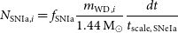 \begin{equation} N_{\mathrm{SNIa}, i} = f_\textrm{SNIa} \frac{m_{\mathrm{WD}, i}}{1.44\,\rm M_\odot} \frac{dt}{t_\textrm{scale, SNeIa}}\end{equation}
A minimum delay time of 10–100 Myr is often implemented to account for the time needed for the first WDs to form after the initial star formation. However, the delay-time-distribution (DTD) of SNe Ia in our model starts from the formation of WDs instead of stars so this minimum delay time is already incorporated into our stellar lifetime calculation. In summary of the timescales of the three major nucleosynthesis channels, CCSNe explode within thirty Myr (one time step), followed by AGBs from intermediate-mass stars over a few Myr years to a few Gyrs, and lastly succeeded by their WD remnants igniting as SNe Ia.
The SFR in our model is computed using the Kennicutt-Schmidt (KS) law (Schmidt Reference Schmidt1959; Kennicutt Reference Kennicutt1998; Kennicutt & Evans Reference Kennicutt and Evans2012), as represented below:
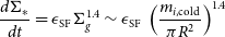 \begin{equation} \frac{d\Sigma_*}{dt} = \epsilon_{\mathrm{SF}} \Sigma_{g}^{1.4} \sim \epsilon_{\mathrm{SF}} \ \left(\frac{m_{i, \mathrm{cold}}}{\pi R^2}\right)^{1.4}\end{equation}
Here, ${m_{i, \mathrm{cold}}}$
represents the quantity of cold ISM available in the box at time step i. The radius of our GCE box is used for calculating the gas density and in turn the SFR in our model. Thus, the radius degenerates with the SFE, which is a free parameter during our exploration. We have set the SFE,
${m_{i, \mathrm{cold}}}$
represents the quantity of cold ISM available in the box at time step i. The radius of our GCE box is used for calculating the gas density and in turn the SFR in our model. Thus, the radius degenerates with the SFE, which is a free parameter during our exploration. We have set the SFE, $\epsilon_{\mathrm{SF}}$
, a free parameter for the star formation mechanism so we decided to fix R. The materials in the model are assumed to be uniformly distributed. The size of the proto-Galaxy could be rapidly changing but constraining it would require some understanding of the rate of chemical evolution. Here we only aim to capture the effects leading to an increase in [
$\epsilon_{\mathrm{SF}}$
, a free parameter for the star formation mechanism so we decided to fix R. The materials in the model are assumed to be uniformly distributed. The size of the proto-Galaxy could be rapidly changing but constraining it would require some understanding of the rate of chemical evolution. Here we only aim to capture the effects leading to an increase in [ $\alpha$
/Fe].
$\alpha$
/Fe].
The newly formed stellar mass is distributed to stellar mass bins following the IMF mentioned previously, and the corresponding amount of cold ISM is locked inside these stars. Upon reaching their stellar lifetimes and releasing the gas enriched by nucleosynthesis, 1% is allocated to the cold ISM, 79% to the warm ISM, and the remaining is assumed to be lost from the model. The warm ISM cools exponentially over a timescale of $t_{\mathrm{cool}}$
, during which a fraction equal to
$t_{\mathrm{cool}}$
, during which a fraction equal to $dt/ t_{\mathrm{cool}}$
is transferred to the cold ISM during each step. The cooling of the warm ISM is performed at the beginning of each time step. The process of star formation and evolutionary events will cause a portion of the cold ISM to transition into warm ISM through feedback. We set the mass loading factors
$dt/ t_{\mathrm{cool}}$
is transferred to the cold ISM during each step. The cooling of the warm ISM is performed at the beginning of each time step. The process of star formation and evolutionary events will cause a portion of the cold ISM to transition into warm ISM through feedback. We set the mass loading factors $\eta_\textrm{SF}$
and
$\eta_\textrm{SF}$
and $\eta_\textrm{SN}$
to 2.0 and 5.0, respectively. The mass loading factors are estimated by Li, Bryan, & Ostriker (Reference Li, Bryan and Ostriker2017), Fox et al. (Reference Fox, Richter, Ashley, Heckman and Lehner2019), Kim et al. (Reference Kim2020), which are typically several times. A quantity of cold ISM, equivalent to
$\eta_\textrm{SN}$
to 2.0 and 5.0, respectively. The mass loading factors are estimated by Li, Bryan, & Ostriker (Reference Li, Bryan and Ostriker2017), Fox et al. (Reference Fox, Richter, Ashley, Heckman and Lehner2019), Kim et al. (Reference Kim2020), which are typically several times. A quantity of cold ISM, equivalent to $\eta$
times the mass of gas involved in these activities, will be instantaneously heated into warm ISM. Finally, during each time step, an influx of fresh infalling gas will replenish the warm ISM.
$\eta$
times the mass of gas involved in these activities, will be instantaneously heated into warm ISM. Finally, during each time step, an influx of fresh infalling gas will replenish the warm ISM.
2.2. Exhaustive parameter exploration
The conventional approach to creating a GCE model that reproduces specific chemical evolutionary tracks involves manually choosing parameter values and coming up with a standard matching model. However, this method demands strong observational constraints to restrict the resulting GCE scenario, such as the age-abundance relations and the stellar density distribution of specific abundances. In the case of the Milky Way disk, we have a large amount of observational data to constrain the large number of parameters in our GCE model. As for the pre-disk prototype Milky Way, our observational data focus on a small number of metal-poor stars. We have little knowledge about the star formation history or the overarching properties of the Galaxy shortly after its birth. As a result, we chose five free parameters that are fundamental in GCE models and ran our model with randomly generated parameter values. The goal is to explore the physical conditions that could have led to the early rapid chemical evolution, specifically the observed [ $\alpha$
/Fe]-rise, with little bias from the users of GCE models. The feasible ranges for these parameters are chosen to encompass the values typically utilized for Milky Way studies. We have also performed test runs to narrow down the parameter ranges to use computational resources more efficiently.
$\alpha$
/Fe]-rise, with little bias from the users of GCE models. The feasible ranges for these parameters are chosen to encompass the values typically utilized for Milky Way studies. We have also performed test runs to narrow down the parameter ranges to use computational resources more efficiently.
The five free parameters in our GCE models are:
-
• the initial mass of cold interstellar medium ISM, $m_{0, \mathrm{cold}}$
;
$m_{0, \mathrm{cold}}$
; -
• the fraction of white dwarfs arising from progenitor stars with initial masses within the range of (3, 8)
$\mathrm{M}_\odot$
, eligible for SNe Ia,
$f_\textrm{SNIa}$
; -
• the cooling timescale of warm ISM,
$t_{\mathrm{cool}}$
; -
• the SFE,
$\epsilon_{\mathrm{SF}}$
; and -
• the inflow rate,
$\dot{m}_{\mathrm{inflow}}$
.


The following is the role each parameter plays and how we chose the ranges of parameters:
-
• The initial mass of the cold ISM,
$m_{0, \mathrm{cold}}$
, sets the recorded value of [Fe/H] after the first round of star formation in the model. We permit it to be between
$10^{8}$
and
$10^{10}$
$\mathrm{M}_\odot$
. Typically, the inflow history takes the form of an exponential function over time in GCE models to simulate the early rapid growth of a galaxy.
$m_{0, \mathrm{cold}}$
represents the mass of cold gas inside a galaxy at its birth and that accreted shortly after its birth. -
• The fraction of Type Ia supernovae,
$f_\textrm{SNIa}$
, is estimated to be around 5% (Maoz, Mannucci, & Brandt Reference Maoz, Mannucci and Brandt2012; Maoz & Mannucci 2017), but the actual proportion remains uncertain at high redshift. We permit it to be between 1% and 10%. This key parameter influences the evolution of [Fe/H] and [
$\alpha$
/Fe] several hundred million years after the initial star formation event when a considerable amount of SNe Ia start producing iron. -
•
$t_{\mathrm{cool}}$
controls the rate at which newly synthesized metal is returned to the cold ISM for star formation and ranges between
$10^8$
to
$10^{10}$
years in our model, based on simulation results from Stevens et al. (2017). Determining a cooling timescale for our warm ISM is challenging because it realistically depends on factors such as temperature and metallicity (Krumholz Reference Krumholz2012). However, it should typically range from a few hundred million years to a few billion years. -
•
$\epsilon_{\mathrm{SF}}$
controls the efficiency of the process through which cold ISM is converted into stars. The SFE constant can be as low as
$10^{-11}$
(approximately 1% per billion years) to cover the possibility of a low SFE scenario and as high as
$10^{-9}$
. Our range includes SFE values estimated by Bigiel et al. (Reference Bigiel, Leroy, Walter, Brinks, de Blok, Madore and Thornley2008) and Leroy et al. (Reference Leroy, Walter, Brinks, Bigiel, de Blok, Madore and Thornley2008) in nearby galaxies -
• The inflow rate introduces fresh gas into the model and ranges between 0 and 10
$\mathrm{M}_\odot$
per year. The current gas inflow rate in the Galaxy ranges from less than one to several
$\mathrm{M}_\odot$
per year (Fox et al. Reference Fox, Richter, Ashley, Heckman and Lehner2019; Clark, Bordoloi, & Fox Reference Clark, Bordoloi and Fox2022). The continuous inflow of fresh gas could hinder the evolution of [Fe/H] but fuels long-term star formation. Changing the composition of the inflow gas could also alter the abundance ratios in the cold ISM and In turn newly formed stars.


The values of the fixed and free parameters are summarized in Table 1. Parameters $m_{0, \mathrm{cold}}$
,
$m_{0, \mathrm{cold}}$
, $t_{\mathrm{cool}}$
, and
$t_{\mathrm{cool}}$
, and $\epsilon_{\mathrm{SF}}$
are chosen from a log-uniform distribution, allowing their effects on log-scale elemental abundances to be better observed. The remaining two parameters are selected from a uniform distribution. The parameter values are drawn independently randomly each time a new run begins without prior memory. In total, our GCE model is run 300 000 times in order to generate the parameter distribution for the observed [
$\epsilon_{\mathrm{SF}}$
are chosen from a log-uniform distribution, allowing their effects on log-scale elemental abundances to be better observed. The remaining two parameters are selected from a uniform distribution. The parameter values are drawn independently randomly each time a new run begins without prior memory. In total, our GCE model is run 300 000 times in order to generate the parameter distribution for the observed [ $\alpha$
/Fe]-rise. However, replicating the [
$\alpha$
/Fe]-rise. However, replicating the [ $\alpha$
/Fe]-rise is not possible if the parameter values remain constant. Once Type Ia supernovae commence, [
$\alpha$
/Fe]-rise is not possible if the parameter values remain constant. Once Type Ia supernovae commence, [ $\alpha$
/Fe] decreases monotonically, necessitating additional
$\alpha$
/Fe] decreases monotonically, necessitating additional $\alpha$
elements through infall or enhanced star formation to reverse the trend. Therefore,
$\alpha$
elements through infall or enhanced star formation to reverse the trend. Therefore, $\epsilon_{\mathrm{SF}}$
and
$\epsilon_{\mathrm{SF}}$
and $\dot{m}_{\mathrm{inflow}}$
are allowed to change during the second phase, along with the composition of the inflow gas.
$\dot{m}_{\mathrm{inflow}}$
are allowed to change during the second phase, along with the composition of the inflow gas.
Table 1. The values of fixed and free parameters in our GCE model.
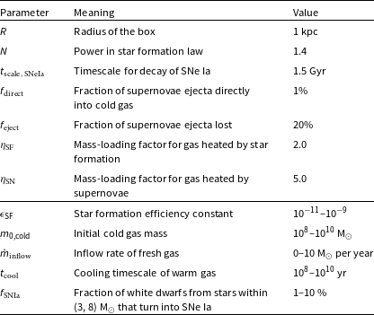
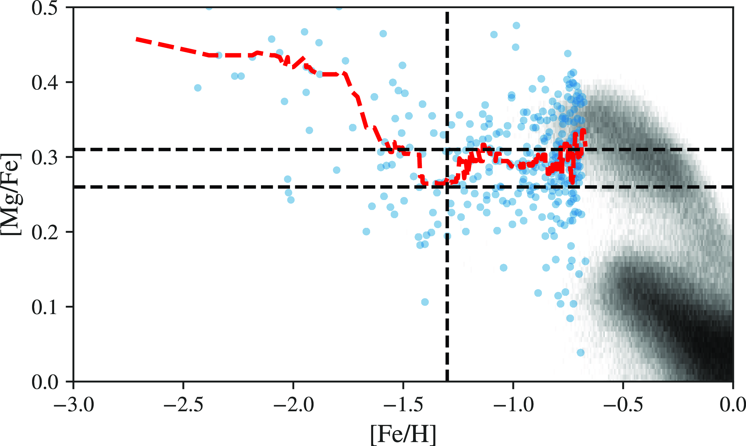
Figure 2. Selected in situ metal-poor stars from the H3 survey in the [Fe/H]-[Mg/Fe]-plane. The stars observed by H3 are shown in blue, and the distribution of stars observed by APOGEE is shown in grey to provide reference of [ $\alpha$
/Fe] values. The moving median of [Mg/Fe] (a red dashed line) is calculated along [Fe/H] with a window size of twenty. The three black dashed lines correspond to three key abundance ratios identified from the median track, [Fe/H] = -1.3, [Mg/Fe] = 0.26, [Mg/Fe] = 0.31.
$\alpha$
/Fe] values. The moving median of [Mg/Fe] (a red dashed line) is calculated along [Fe/H] with a window size of twenty. The three black dashed lines correspond to three key abundance ratios identified from the median track, [Fe/H] = -1.3, [Mg/Fe] = 0.26, [Mg/Fe] = 0.31.
Our model incorporates two mechanisms for producing additional $\alpha$
elements. The first mechanism operates through an increase in the star formation efficiency (SFE). If there is enough cold ISM to support star formation, a rapid rise in SFE can result in a substantial number of CCSN in a short period. Without sufficient cold ISM, however, the model depletes its existing cold ISM, ceasing further star formation. The second mechanism involves gas accretion into the model. A significant challenge with this method is determining the chemical composition of the accreted gas. We utilized a separate GCE model with identical parameters except for
$\alpha$
elements. The first mechanism operates through an increase in the star formation efficiency (SFE). If there is enough cold ISM to support star formation, a rapid rise in SFE can result in a substantial number of CCSN in a short period. Without sufficient cold ISM, however, the model depletes its existing cold ISM, ceasing further star formation. The second mechanism involves gas accretion into the model. A significant challenge with this method is determining the chemical composition of the accreted gas. We utilized a separate GCE model with identical parameters except for $f_{\text{SNIa}}$
set to zero, providing a source of high-[
$f_{\text{SNIa}}$
set to zero, providing a source of high-[ $\alpha$
/Fe] gas for inflow. We synchronized the metallicities of the inflow gas with that of the existing gas within the model to ensure no break in metallicity. Despite the absence of contributions from Type Ia supernovae in the accompanying model, its [Mg/Fe] declines due to metallicity-dependent yields. Specifically, [Mg/Fe] decreases from a maximum of 0.52 at zero metallicity to 0.42 at [Fe/H]
$\alpha$
/Fe] gas for inflow. We synchronized the metallicities of the inflow gas with that of the existing gas within the model to ensure no break in metallicity. Despite the absence of contributions from Type Ia supernovae in the accompanying model, its [Mg/Fe] declines due to metallicity-dependent yields. Specifically, [Mg/Fe] decreases from a maximum of 0.52 at zero metallicity to 0.42 at [Fe/H] $\approx -1.3$
. As [Fe/H] increases from
$\approx -1.3$
. As [Fe/H] increases from $-1.3$
to
$-1.3$
to $-0.9$
, [Mg/Fe] in the inflow gas further reduces to 0.3. With this method, the incoming gas not only directly provides additional
$-0.9$
, [Mg/Fe] in the inflow gas further reduces to 0.3. With this method, the incoming gas not only directly provides additional $\alpha$
-elements but also promotes the short-term generation of CCSNe through heightened star formation activity. This [
$\alpha$
-elements but also promotes the short-term generation of CCSNe through heightened star formation activity. This [ $\alpha$
/Fe]-enhanced inflow gas is only implemented at the beginning of the second phase of the chemical evolution, before which the inflow gas remains pristine.
$\alpha$
/Fe]-enhanced inflow gas is only implemented at the beginning of the second phase of the chemical evolution, before which the inflow gas remains pristine.

Figure 3. The aggregate effect of the five free parameters on the chemical evolutionary tracks. Each panel represents one free parameter in the GCE model. The SFE ( $\epsilon_{\mathrm{SF}}$
) and inflow rate (
$\epsilon_{\mathrm{SF}}$
) and inflow rate ( $\dot{m}_\textrm{inflow}$
) are allowed to change after one Gyr when we expect [
$\dot{m}_\textrm{inflow}$
) are allowed to change after one Gyr when we expect [ $\alpha$
/Fe] to reverse and thus represented in two panels, respectively, before and after the turning point. Each panel contains four tracks averaged across [Mg/Fe] within the four quartiles of the parameter range. The median value of each parameter is shown in the legend with the corresponding colour and line style. As the rest of the parameters are drawn randomly in each run, the effect of the other parameters is expected to even out, allowing us to observe the effect of a single parameter.
$\alpha$
/Fe] to reverse and thus represented in two panels, respectively, before and after the turning point. Each panel contains four tracks averaged across [Mg/Fe] within the four quartiles of the parameter range. The median value of each parameter is shown in the legend with the corresponding colour and line style. As the rest of the parameters are drawn randomly in each run, the effect of the other parameters is expected to even out, allowing us to observe the effect of a single parameter.
The task remains to select the tracks that fit the observed chemical trend after the models are run. We identify three key elemental abundances from the H3 in situ sample to characterize the [Fe/H]-[ $\alpha$
/Fe]-track we aim to reproduce. Fig. 2 shows the H3 in situ sample in the [Fe/H]-[Mg/Fe] plane. The distribution of the disk population from APOGEE DR17 is shown in grey in the background to provide a reference for [Mg/Fe] values. A moving median-[Mg/Fe] track (in a red dashed line) is fitted to the sample along [Fe/H] with a window size of twenty to reveal the trend in [Mg/Fe]. The three black dashed lines correspond to the three key elemental abundances from the [Mg/Fe]-trend: 1) [Fe/H] = -1.3 where [Mg/Fe] reached the lowest value; 2) [Mg/Fe] = 0.26, the lowest value [Mg/Fe] reached around [Fe/H] = -1.3; 3) [Mg/Fe] = 0.31, the [Mg/Fe] value joining the thick disk population in the chemical space. We will design our selection criteria based on these abundances below.
$\alpha$
/Fe]-track we aim to reproduce. Fig. 2 shows the H3 in situ sample in the [Fe/H]-[Mg/Fe] plane. The distribution of the disk population from APOGEE DR17 is shown in grey in the background to provide a reference for [Mg/Fe] values. A moving median-[Mg/Fe] track (in a red dashed line) is fitted to the sample along [Fe/H] with a window size of twenty to reveal the trend in [Mg/Fe]. The three black dashed lines correspond to the three key elemental abundances from the [Mg/Fe]-trend: 1) [Fe/H] = -1.3 where [Mg/Fe] reached the lowest value; 2) [Mg/Fe] = 0.26, the lowest value [Mg/Fe] reached around [Fe/H] = -1.3; 3) [Mg/Fe] = 0.31, the [Mg/Fe] value joining the thick disk population in the chemical space. We will design our selection criteria based on these abundances below.
3. Results
Before we dig into the [ $\alpha$
/Fe]-rise, we will look at each parameter to understand its effect on the chemical tracks. Fig. 3 shows the median tracks for the four quartiles of each parameter value within its range. Since
$\alpha$
/Fe]-rise, we will look at each parameter to understand its effect on the chemical tracks. Fig. 3 shows the median tracks for the four quartiles of each parameter value within its range. Since $\epsilon_{\mathrm{SF}}$
and
$\epsilon_{\mathrm{SF}}$
and $\dot{m}_{\mathrm{inflow}}$
are allowed to change after [
$\dot{m}_{\mathrm{inflow}}$
are allowed to change after [ $\alpha$
/Fe] reaches the lowest value, there are two panels for each of these two parameters to showcase the tracks before and after the change. For each parameter in question, we divide its parameter values into four quartiles and obtain a median track over [
$\alpha$
/Fe] reaches the lowest value, there are two panels for each of these two parameters to showcase the tracks before and after the change. For each parameter in question, we divide its parameter values into four quartiles and obtain a median track over [ $\alpha$
/Fe] for models in each quartile. We refer to the point where [
$\alpha$
/Fe] for models in each quartile. We refer to the point where [ $\alpha$
/Fe] reaches the lowest value in the [Fe/H]-[
$\alpha$
/Fe] reaches the lowest value in the [Fe/H]-[ $\alpha$
/Fe]-plane as the [Fe/H]-[
$\alpha$
/Fe]-plane as the [Fe/H]-[ $\alpha$
/Fe]-knee, which divides the chemical evolutionary history we study into two phases. Here are the main observations from Fig. 3:
$\alpha$
/Fe]-knee, which divides the chemical evolutionary history we study into two phases. Here are the main observations from Fig. 3:
-
• All of the median tracks exhibit elevated or stable [Mg/Fe] during the second phase of the evolution. This pattern is anticipated following a sudden alteration in the chemical composition of the inflow gas from pristine to [
$\alpha$
/Fe]-enhanced. Furthermore, the extent of the increase in [Mg/Fe] depends on the magnitude of changes in the updated parameters. -
• Increasing the initial mass of cold ISM results in a [Fe/H]-[
$\alpha$
/Fe]-knee that is higher in [Fe/H] and lower in [
$\alpha$
/Fe]. Models with more massive initial cold ISM experience have a stronger initial burst of star formation and thus reach a higher starting metallicity. More active initial star formation also translates to more early SNe Ia, causing [
$\alpha$
/Fe] to decline sooner. This is evidenced by the lower [
$\alpha$
/Fe] as the initial mass increases. -
• Increasing
$f_{\mathrm{SNIa}}$
results in a [Fe/H]-[
$\alpha$
/Fe]-knee that is lower in [
$\alpha$
/Fe] and slightly higher in [Fe/H]. A star with an initial mass of ten
$\mathrm{M}_\odot$
will produce about 0.05
$\mathrm{M}_\odot$
of Mg as it explodes as a CCSN, but a single SNIa produces about 0.7
$\mathrm{M}_\odot$
of Fe. A small increase in
$f_{\mathrm{SNIa}}$
leads to more SNe Ia and a large difference in [
$\alpha$
/Fe]. -
• Increasing
$\epsilon_{\mathrm{SF}}$
during the first phase results in a [Fe/H]-[
$\alpha$
/Fe]-knee that is higher in [Fe/H] and lower in [
$\alpha$
/Fe]. Models with a higher SFE transform cold ISM into stars and in turn metals more efficiently and thus are more capable of reaching high [Fe/H]. The more efficient star formation also leads to more early SNe Ia and causes more iron to be produced sooner when given the same gas accretion history. -
•
$\epsilon_{\mathrm{SF}}$
during the second phase affects the amount of increase in [
$\alpha$
/Fe] and [Fe/H] during the second phase. The values of
$\epsilon_{\mathrm{SF}}$
before and after the [Fe/H]-[
$\alpha$
/Fe]-knee are independent as both are randomly chosen. Models with insufficient gas to sustain high SFEs tend to cause errors in our model and thus are not present here. As long as there is sufficient gas, a high SFE translates to a stronger star formation burst to achieve quick chemical evolution. -
• Inflow rate before the [Fe/H]-[
$\alpha$
/Fe]-knee has no significant effect on the tracks in the [Fe/H]-[
$\alpha$
/Fe]-plane, except when it is very small. The elemental abundances reflect the balances of nucleosynthesis channels. Inflow during the first phase only indirectly affects these channels by influencing the SFH. When the inflow rate is reasonably high, the SFE or
$f_{\mathrm{SNIa}}$
could be low so the star formation activity is suppressed. However, when
$\dot{m}_{\mathrm{inflow, before}}$
is very small, the GCE model can be treated as a closed box and thus its chemical enrichment is more effective, evidenced by the higher [Fe/H] and lower [Mg/Fe] of the blue track. -
• Inflow rate after the [Fe/H]-[
$\alpha$
/Fe]-knee affects how high [
$\alpha$
/Fe] can rise during the second phase. The sudden arrival of accreted gas brings in additional
$\alpha$
elements and causes a large number of massive stars to form and evolve over a short time, reversing the declining trend of [
$\alpha$
/Fe]. -
• The cooling time controls the rate of gas recycling and in turn the rate of chemical evolution. The metallicity value of the [Fe/H]-[
$\alpha$
/Fe]-knee moves up as the cooling time is reduced. However, gas cooling has little effect on [
$\alpha$
/Fe], unlike star formation parameters.


Based on these observations, we can expect models that match the observed [Fe/H]-[ $\alpha$
/Fe]-track to have relatively high initial mass and SFE, intermediate values of
$\alpha$
/Fe]-track to have relatively high initial mass and SFE, intermediate values of $f_{\mathrm{SNIa}}$
and
$f_{\mathrm{SNIa}}$
and $t_{\mathrm{cool}}$
, and raised SFE as well as inflow rate during the second phase to boost
$t_{\mathrm{cool}}$
, and raised SFE as well as inflow rate during the second phase to boost $\alpha$
production. We create three selection criteria based on the abundance ratios from Fig. 2 to isolate models that replicate the rise in [Mg/Fe]:
$\alpha$
production. We create three selection criteria based on the abundance ratios from Fig. 2 to isolate models that replicate the rise in [Mg/Fe]:
-
• should reach
$-1.3 \pm 0.05$
dex after one Gyr; -
• should reach
$0.26 \pm 0.05$
dex after one Gyr; -
• [Fe/H] should reach above -0.9, [Mg/Fe] should rise above 0.3, and the increase of [Mg/Fe] should exceed 0.05 dex at any point during the second Gyr.


The abundances have a large spread in this part of the [Fe/H]-[ $\alpha$
/Fe]-plane so it is difficult to pinpoint the exact key abundance ratios. We leave a margin (0.05 dex) for [Fe/H] and [Mg/Fe] to account for the possible spread in the abundances. The target [Fe/H] and [Mg/Fe] at the end of the two Gyr are chosen to match the metal-poor end of the high-[
$\alpha$
/Fe]-plane so it is difficult to pinpoint the exact key abundance ratios. We leave a margin (0.05 dex) for [Fe/H] and [Mg/Fe] to account for the possible spread in the abundances. The target [Fe/H] and [Mg/Fe] at the end of the two Gyr are chosen to match the metal-poor end of the high-[ $\alpha$
/Fe] thick disk. Fig. 4 shows the density distribution of tracks in [Fe/H]-[Mg/Fe] when each criterion is incrementally applied to all of the tracks generated from within our parameter space. The black dashed lines mark the key abundance ratios identified from Fig. 2, and the black dotted line marks the [Mg/Fe] value of the inflow gas during the second phase. In the top panel, only condition (1) is applied and 14 017 tracks (4.7% of the total number of runs) remain after the selection. The tracks significantly diverge after [Fe/H]=-2.5 when iron from SNe Ia starts to influence [Mg/Fe]. The middle and bottom panels of Fig. 4 show the distribution of tracks in [Fe/H]-[Mg/Fe] when the first two criteria and all three are applied, respectively. There are 6 174 tracks (2.1%) in the middle panel and only 735 (0.25%) in the bottom. We will walk through the main results from each criterion that is subsequently applied in the following sections in order. For reference, we tested our models with low-[
$\alpha$
/Fe] thick disk. Fig. 4 shows the density distribution of tracks in [Fe/H]-[Mg/Fe] when each criterion is incrementally applied to all of the tracks generated from within our parameter space. The black dashed lines mark the key abundance ratios identified from Fig. 2, and the black dotted line marks the [Mg/Fe] value of the inflow gas during the second phase. In the top panel, only condition (1) is applied and 14 017 tracks (4.7% of the total number of runs) remain after the selection. The tracks significantly diverge after [Fe/H]=-2.5 when iron from SNe Ia starts to influence [Mg/Fe]. The middle and bottom panels of Fig. 4 show the distribution of tracks in [Fe/H]-[Mg/Fe] when the first two criteria and all three are applied, respectively. There are 6 174 tracks (2.1%) in the middle panel and only 735 (0.25%) in the bottom. We will walk through the main results from each criterion that is subsequently applied in the following sections in order. For reference, we tested our models with low-[ $\alpha$
/Fe] inflow gas that shares [
$\alpha$
/Fe] inflow gas that shares [ $\alpha$
/Fe] with existing cold ISM and less than ten models passed the three criteria from the same number of runs.
$\alpha$
/Fe] with existing cold ISM and less than ten models passed the three criteria from the same number of runs.
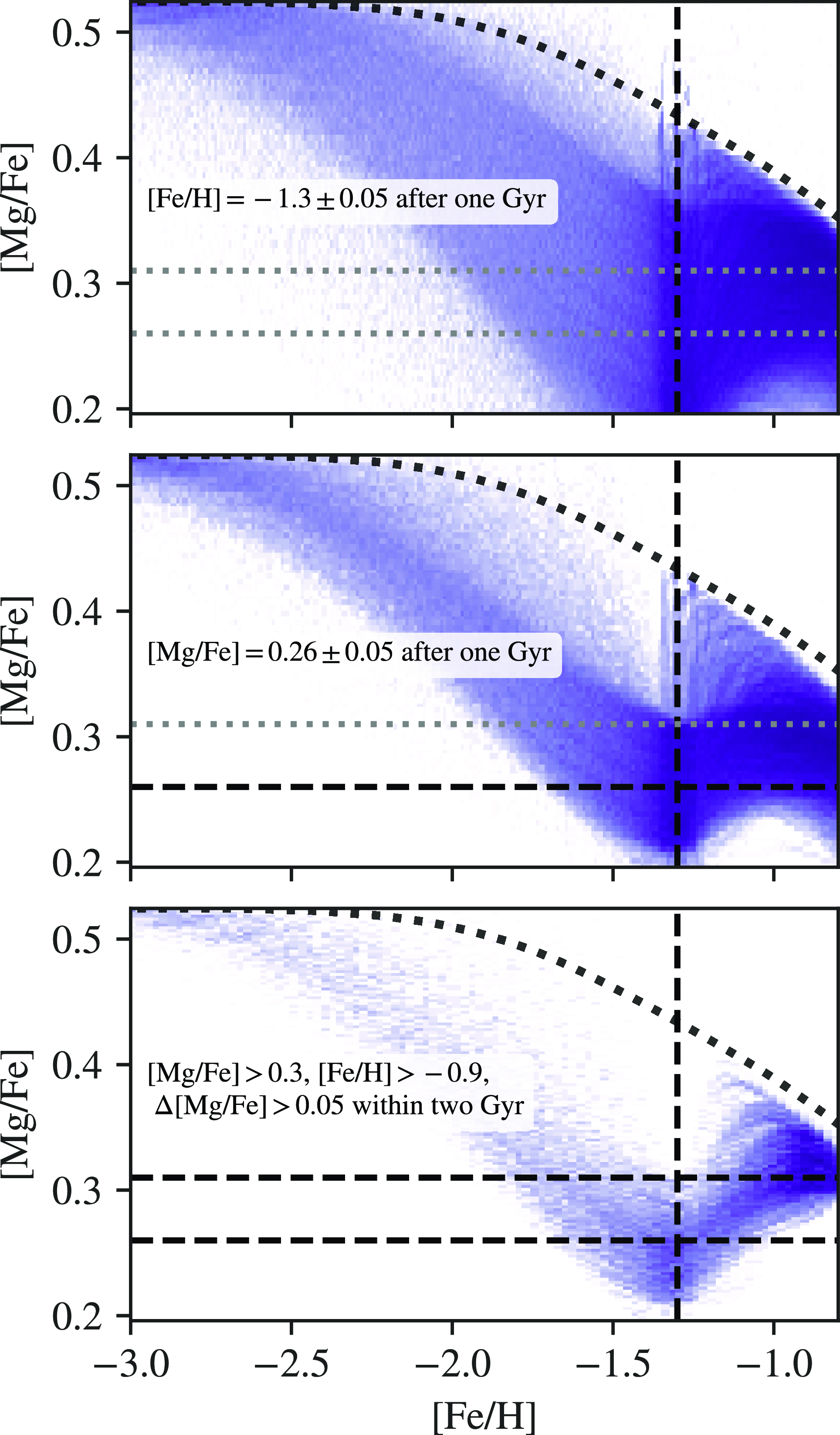
Figure 4. The density distribution of chemical evolutionary tracks after each selection criterion is incrementally applied to the results of our GCE runs. Tracks in the top panel reach [Fe/H] of $-1.3 \pm 0.05$
after one Gyr. Tracks in the middle panel reach [Mg/Fe] of
$-1.3 \pm 0.05$
after one Gyr. Tracks in the middle panel reach [Mg/Fe] of $0.26 \pm 0.05$
after one Gyr in addition. Tracks in the bottom panel are capable of reaching [Fe/H] = -0.9 and [Mg/Fe]
$0.26 \pm 0.05$
after one Gyr in addition. Tracks in the bottom panel are capable of reaching [Fe/H] = -0.9 and [Mg/Fe] $> 0.3$
as well as achieving an increase of at least 0.05 dex in [Mg/Fe]. The black dotted track marks [Mg/Fe] of the parallel model with no SNe Ia, from which inflow gas takes its composition after [Mg/Fe] reaches the lowest point. The straight and vertical lines correspond to three key abundance ratios identified from the median [Mg/Fe]-trend in Fig. 2, each of which becomes highlighted when the corresponding selection criterion is applied.
$> 0.3$
as well as achieving an increase of at least 0.05 dex in [Mg/Fe]. The black dotted track marks [Mg/Fe] of the parallel model with no SNe Ia, from which inflow gas takes its composition after [Mg/Fe] reaches the lowest point. The straight and vertical lines correspond to three key abundance ratios identified from the median [Mg/Fe]-trend in Fig. 2, each of which becomes highlighted when the corresponding selection criterion is applied.
3.1. The target [Fe/H] sets the basic conditions
Fig. 5 displays the distribution of free parameter values ( $m_{0, \mathrm{cold}}$
,
$m_{0, \mathrm{cold}}$
, $f_\textrm{SNIa}$
,
$f_\textrm{SNIa}$
, $t_{\mathrm{cool}}$
,
$t_{\mathrm{cool}}$
, $\epsilon_{\mathrm{SF}}$
,
$\epsilon_{\mathrm{SF}}$
, $\dot{m}_{\mathrm{inflow}}$
) of the models that satisfy the first criterion ([Fe/H] =
$\dot{m}_{\mathrm{inflow}}$
) of the models that satisfy the first criterion ([Fe/H] = $-1.3 \pm 0.05$
after one Gyr). The diagonal panels show one-dimensional histograms of the free parameters, while the off-diagonal panels feature the joint distribution smoothed by kernel density estimations. The values for
$-1.3 \pm 0.05$
after one Gyr). The diagonal panels show one-dimensional histograms of the free parameters, while the off-diagonal panels feature the joint distribution smoothed by kernel density estimations. The values for $\epsilon_{\mathrm{SF}}$
and
$\epsilon_{\mathrm{SF}}$
and $\dot{m}_{\mathrm{inflow}}$
in the ‘simmering’ phase scenario from Conroy et al. (Reference Conroy2022) are highlighted. In each of the off-diagonal panels, we add a solid line resulting from a linear regression fit and dashed lines to demonstrate the residual from the fit. The lines are for illustrative purposes only and do not necessarily indicate actual correlations among the parameters. The parameter space does not satisfy the assumptions for a linear regression analysis. Examining the diagonal histograms, no preference emerges for
$\dot{m}_{\mathrm{inflow}}$
in the ‘simmering’ phase scenario from Conroy et al. (Reference Conroy2022) are highlighted. In each of the off-diagonal panels, we add a solid line resulting from a linear regression fit and dashed lines to demonstrate the residual from the fit. The lines are for illustrative purposes only and do not necessarily indicate actual correlations among the parameters. The parameter space does not satisfy the assumptions for a linear regression analysis. Examining the diagonal histograms, no preference emerges for $f_\textrm{SNIa}$
and
$f_\textrm{SNIa}$
and $\epsilon_{\mathrm{SF}}$
as their distribution remains uniform, while preferences for
$\epsilon_{\mathrm{SF}}$
as their distribution remains uniform, while preferences for $m_{0, \mathrm{cold}} \sim 10^{10}$ $\mathrm{M}_\odot$
and
$\mathrm{M}_\odot$
and $t_{\mathrm{cool}} \sim 10^{8.5}$
yr are apparent. As we have seen in Fig. 3, models with a low SFE are unlikely to produce enough iron to meet the desired [Fe/H] at the [Fe/H]-[
$t_{\mathrm{cool}} \sim 10^{8.5}$
yr are apparent. As we have seen in Fig. 3, models with a low SFE are unlikely to produce enough iron to meet the desired [Fe/H] at the [Fe/H]-[ $\alpha$
/Fe]-knee as we have very few models with an SFE less than
$\alpha$
/Fe]-knee as we have very few models with an SFE less than $10^{-10.5}$
.
$10^{-10.5}$
.
Some correlations between the remaining values of the free parameters become evident when inspecting the joint distributions. $m_{0, \mathrm{cold}}$
, represented in the first column, determines the initial amount of star formation and consequently [Fe/H] after the first step in the model. There is no visible correlation
$m_{0, \mathrm{cold}}$
, represented in the first column, determines the initial amount of star formation and consequently [Fe/H] after the first step in the model. There is no visible correlation $m_{0, \mathrm{cold}}$
and
$m_{0, \mathrm{cold}}$
and $f_\textrm{SNIa}$
, but we can see a positive correlation between
$f_\textrm{SNIa}$
, but we can see a positive correlation between $m_{0, \mathrm{cold}}$
and
$m_{0, \mathrm{cold}}$
and $t_{\mathrm{cool}}$
when
$t_{\mathrm{cool}}$
when $m_{0, \mathrm{cold}}$
exceeds
$m_{0, \mathrm{cold}}$
exceeds $10^{8.5}$ $\mathrm{M}_\odot$
. Given that we set the power in the Kennicutt-Schmidt law to
$\mathrm{M}_\odot$
. Given that we set the power in the Kennicutt-Schmidt law to $1.4$
, a larger volume of cold ISM results in a proportionally larger increase in SFR, thereby affecting the amount of metal produced in the first step. If too much metal is produced, the cooling time of the warm ISM needs to be extended accordingly to prevent [Fe/H] from surpassing our target. When
$1.4$
, a larger volume of cold ISM results in a proportionally larger increase in SFR, thereby affecting the amount of metal produced in the first step. If too much metal is produced, the cooling time of the warm ISM needs to be extended accordingly to prevent [Fe/H] from surpassing our target. When $m_{0, \mathrm{cold}}$
falls below
$m_{0, \mathrm{cold}}$
falls below $10^{8.5}$ $\mathrm{M}_\odot$
, the slope is less steep because the amount of metal produced from the initial reservoir is not massive enough to require additional cooling; in this case, the [Fe/H] progression rate can be modulated by other parameters.
$\mathrm{M}_\odot$
, the slope is less steep because the amount of metal produced from the initial reservoir is not massive enough to require additional cooling; in this case, the [Fe/H] progression rate can be modulated by other parameters.
Further down the first column, the fitted line between $m_{0, \mathrm{cold}}$
and
$m_{0, \mathrm{cold}}$
and $\epsilon_{\mathrm{SF}}$
indicates a negative correlation, but this is false and only reflects the cut-off of models unable to reach the metallicity target in parameter space. Contrary to the cooling timescale which delays the return of metals into the cold ISM, a high SFE accelerates the conversion of cold ISM into stars and in turn metals within the model. When a massive reservoir of cold ISM (high
$\epsilon_{\mathrm{SF}}$
indicates a negative correlation, but this is false and only reflects the cut-off of models unable to reach the metallicity target in parameter space. Contrary to the cooling timescale which delays the return of metals into the cold ISM, a high SFE accelerates the conversion of cold ISM into stars and in turn metals within the model. When a massive reservoir of cold ISM (high $m_{0, \mathrm{cold}}$
) is initially present in the model, the metallicity after one step of star formation is higher and thus the SFE has a large degree of flexibility as the chemical evolution could be modulated by other parameters. Conversely, with an insignificant initial mass of cold ISM (low
$m_{0, \mathrm{cold}}$
) is initially present in the model, the metallicity after one step of star formation is higher and thus the SFE has a large degree of flexibility as the chemical evolution could be modulated by other parameters. Conversely, with an insignificant initial mass of cold ISM (low $m_{0, \mathrm{cold}}$
) forces a dependency on infall to accumulate cold ISM, a high SFE is necessary to facilitate the increase in [Fe/H] over the first one Gyr to reach our [Fe/H] target in time.
$m_{0, \mathrm{cold}}$
) forces a dependency on infall to accumulate cold ISM, a high SFE is necessary to facilitate the increase in [Fe/H] over the first one Gyr to reach our [Fe/H] target in time.
The bottom panel on the first column again shows where the parameters cut-off between $m_{0, \mathrm{cold}}$
and
$m_{0, \mathrm{cold}}$
and $\dot{m}_{\mathrm{inflow}}$
. Star formation only converts a few percentages of cold ISM into stars per Gyr, resulting in only a minuscule amount of metal production relative to the amount of inflow gas. Quantitatively, based on the nucleosynthesis tables and the IMF we utilized, every solar mass of core-collapse supernova (CCSN), the primary production site of iron before the onset of SNe Ia, produces about
$\dot{m}_{\mathrm{inflow}}$
. Star formation only converts a few percentages of cold ISM into stars per Gyr, resulting in only a minuscule amount of metal production relative to the amount of inflow gas. Quantitatively, based on the nucleosynthesis tables and the IMF we utilized, every solar mass of core-collapse supernova (CCSN), the primary production site of iron before the onset of SNe Ia, produces about $6.3 \times 10^{-4}$ $\mathrm{M}_\odot$
of iron. The inflow gas during the first one Gyr is assumed to be pristine. As the cold ISM reservoir is much less massive at this time, even a few
$\mathrm{M}_\odot$
of iron. The inflow gas during the first one Gyr is assumed to be pristine. As the cold ISM reservoir is much less massive at this time, even a few $\mathrm{M}_\odot$
of pristine gas per year can significantly dilute the metal present in the model. Hence, infalling gas primarily inhibits the increase of [Fe/H] at this time. When
$\mathrm{M}_\odot$
of pristine gas per year can significantly dilute the metal present in the model. Hence, infalling gas primarily inhibits the increase of [Fe/H] at this time. When $m_{0, \mathrm{cold}}$
is high and the early star formation burst launches [Fe/H] at a higher value, the inflow rate escalates correspondingly to decelerate the evolution of [Fe/H] subsequently.
$m_{0, \mathrm{cold}}$
is high and the early star formation burst launches [Fe/H] at a higher value, the inflow rate escalates correspondingly to decelerate the evolution of [Fe/H] subsequently.
There seems to be a positive correlation between $t_{\mathrm{cool}}$
and
$t_{\mathrm{cool}}$
and $\epsilon_{\mathrm{SF}}$
, which our linear fit failed to capture due to the existence of models with
$\epsilon_{\mathrm{SF}}$
, which our linear fit failed to capture due to the existence of models with $t_{\mathrm{cool}} > $
one Gyr. To reach the same [Fe/H], the higher the SFE we adopt for the model, the longer we need to store the nucleosynthesis yields so that the same amount of metals are recycled into the cold ISM. This relationship only extends to
$t_{\mathrm{cool}} > $
one Gyr. To reach the same [Fe/H], the higher the SFE we adopt for the model, the longer we need to store the nucleosynthesis yields so that the same amount of metals are recycled into the cold ISM. This relationship only extends to $t_{\mathrm{cool}}$
as high as around one Gyr. When the cooling timescale is longer than one Gyr, the model is forced to adopt a high SFE and regulate the chemical evolution with other parameters. The joint distributions in the remaining panels do not show any significant relationship. Although SNe Ia are typically analogous to iron production when we are studying the chemical evolution in the Milky Way disk, they have a substantial delay time and do not have any significant impact on [Fe/H] during this phase. The slope of the fitted line between
$t_{\mathrm{cool}}$
as high as around one Gyr. When the cooling timescale is longer than one Gyr, the model is forced to adopt a high SFE and regulate the chemical evolution with other parameters. The joint distributions in the remaining panels do not show any significant relationship. Although SNe Ia are typically analogous to iron production when we are studying the chemical evolution in the Milky Way disk, they have a substantial delay time and do not have any significant impact on [Fe/H] during this phase. The slope of the fitted line between $t_{\mathrm{cool}}$
and
$t_{\mathrm{cool}}$
and $\dot{m}_{\mathrm{inflow}}$
is a result of the parameter cutoff when
$\dot{m}_{\mathrm{inflow}}$
is a result of the parameter cutoff when $t_{\mathrm{cool}}$
exceeds one Gyr. When metals in the model take too long to return to the cold ISM, inflow gas would dilute the metals in the cold ISM further and thus needs to be contained to low numbers.
$t_{\mathrm{cool}}$
exceeds one Gyr. When metals in the model take too long to return to the cold ISM, inflow gas would dilute the metals in the cold ISM further and thus needs to be contained to low numbers.
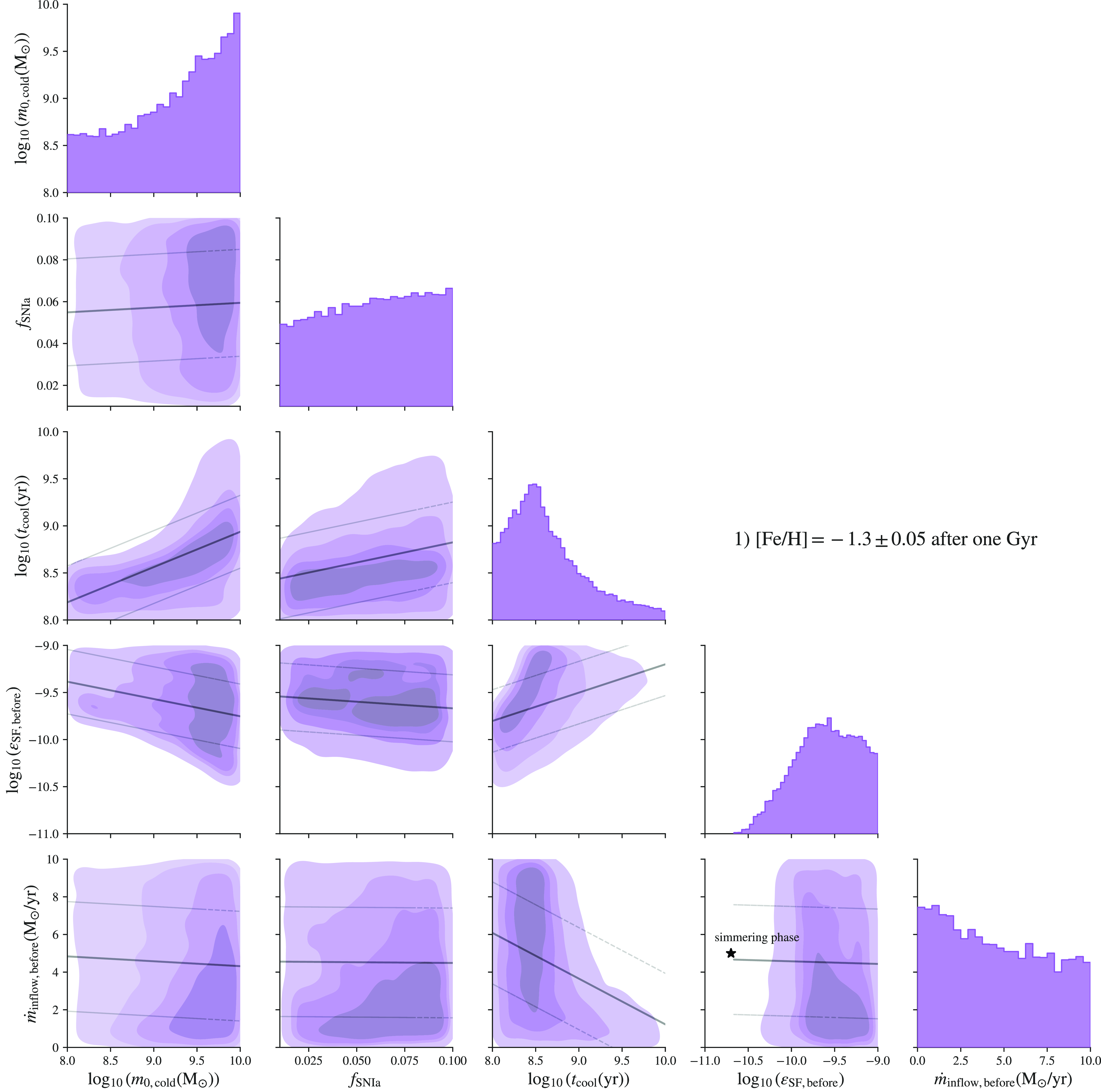
Figure 5. The distribution of parameter values of the models that reach [Fe/H] = $-1.3 \pm 0.05$
after one Gyr. The distribution of tracks generated with these parameter values in [Fe/H]-[Mg/Fe] is shown in the top panel of Fig. 4. The columns and rows correspond to five free parameters in the bottom cell of Table 1, i.e. the initial mass of cold ISM (
$-1.3 \pm 0.05$
after one Gyr. The distribution of tracks generated with these parameter values in [Fe/H]-[Mg/Fe] is shown in the top panel of Fig. 4. The columns and rows correspond to five free parameters in the bottom cell of Table 1, i.e. the initial mass of cold ISM ( $m_{0, \mathrm{cold}}$
), the fraction of white dwarfs arising from progenitor stars with initial masses within the range of (3.2, 8.5)
$m_{0, \mathrm{cold}}$
), the fraction of white dwarfs arising from progenitor stars with initial masses within the range of (3.2, 8.5) $\mathrm{M}_\odot$
eligible for SNe Ia (
$\mathrm{M}_\odot$
eligible for SNe Ia ( $f_\textrm{SNIa}$
), the cooling timescale of warm ISM (
$f_\textrm{SNIa}$
), the cooling timescale of warm ISM ( $t_{\mathrm{cool}}$
), the SFE constant (
$t_{\mathrm{cool}}$
), the SFE constant ( $\epsilon_{\mathrm{SF}}$
), the inflow rate (
$\epsilon_{\mathrm{SF}}$
), the inflow rate ( $\dot{m}_{\mathrm{inflow}}$
). We only show the values of the last two parameters before the [
$\dot{m}_{\mathrm{inflow}}$
). We only show the values of the last two parameters before the [ $\alpha$
/Fe]-rise here. The diagonal panels are one-dimensional histograms for each free parameter and the off-diagonal terms are two-dimensional joint distributions between the parameters smoothed by kernel density estimations. The constant inflow rate and the initial SFE of the ‘simmering’ phase scenario are marked for reference.
$\alpha$
/Fe]-rise here. The diagonal panels are one-dimensional histograms for each free parameter and the off-diagonal terms are two-dimensional joint distributions between the parameters smoothed by kernel density estimations. The constant inflow rate and the initial SFE of the ‘simmering’ phase scenario are marked for reference.


In conclusion, our requirement that [Fe/H] should reach $-1.3 \pm 0.05$
dex in one Gyr selectively favours models featuring a substantial initial cold ISM reservoir (
$-1.3 \pm 0.05$
dex in one Gyr selectively favours models featuring a substantial initial cold ISM reservoir ( $m_{0, \mathrm{cold}} > 10^9$ $\mathrm{M}_\odot$
), a moderate cooling timescale for the warm ISM (
$\mathrm{M}_\odot$
), a moderate cooling timescale for the warm ISM ( $t_{\mathrm{cool}} \approx 10^{8.5} \mathrm{yr}$
), and a relatively elevated SFE (
$t_{\mathrm{cool}} \approx 10^{8.5} \mathrm{yr}$
), and a relatively elevated SFE ( $\epsilon_{\mathrm{SF}} > 10^{-10}$
). The boundaries in the parameter space reflect how some of the parameters compensate each other, such as in the case of
$\epsilon_{\mathrm{SF}} > 10^{-10}$
). The boundaries in the parameter space reflect how some of the parameters compensate each other, such as in the case of $m_{0, \mathrm{cold}}$
and
$m_{0, \mathrm{cold}}$
and $\epsilon_{\mathrm{SF, before}}$
as well as
$\epsilon_{\mathrm{SF, before}}$
as well as $\dot{m}_{\mathrm{inflow, before}}$
. When one parameter takes on an extreme value, it could significantly limit the choice for another.
$\dot{m}_{\mathrm{inflow, before}}$
. When one parameter takes on an extreme value, it could significantly limit the choice for another.
3.2. The frequency of SNe Ia controls the fall of [
$\alpha$
/Fe]

We now explore the parameter space when an additional criterion is imposed on [Mg/Fe]. Models whose parameter distributions are displayed in orange in Fig. 6 are required to hit both [Fe/H] $= -1.3 \pm 0.05$
dex and [Mg/Fe]
$= -1.3 \pm 0.05$
dex and [Mg/Fe] $= 0.26 \pm 0.05$
dex at the one Gyr mark. As expected, characteristics identified in Fig. 5 reappear in Fig. 6. However, some novel features emerge in the new parameter space, notably with
$= 0.26 \pm 0.05$
dex at the one Gyr mark. As expected, characteristics identified in Fig. 5 reappear in Fig. 6. However, some novel features emerge in the new parameter space, notably with $f_\textrm{SNIa}$
, the parameter controlling the frequency of SNe Ia. The value of
$f_\textrm{SNIa}$
, the parameter controlling the frequency of SNe Ia. The value of $f_\textrm{SNIa}$
is constrained to between 3% and 7%. Unlike the rest of the free parameters that affect all nucleosynthesis channels,
$f_\textrm{SNIa}$
is constrained to between 3% and 7%. Unlike the rest of the free parameters that affect all nucleosynthesis channels, $f_\textrm{SNIa}$
only targets SNe Ia. Since a single SNIa produces significantly more iron than the amount of magnesium from a single CCSN,
$f_\textrm{SNIa}$
only targets SNe Ia. Since a single SNIa produces significantly more iron than the amount of magnesium from a single CCSN, $f_\textrm{SNIa}$
essentially dictates the rate of evolution for [Mg/Fe]. Traditionally, GCE models for the Milky Way allow several Gyr for the [
$f_\textrm{SNIa}$
essentially dictates the rate of evolution for [Mg/Fe]. Traditionally, GCE models for the Milky Way allow several Gyr for the [ $\alpha$
/Fe] ratio to drop to replicate a high-[
$\alpha$
/Fe] ratio to drop to replicate a high-[ $\alpha$
/Fe] population that is between eight and ten Gyr old. However, given only one Gyr for [Mg/Fe] to drop from the ceiling to 0.26 in our model, it is interesting that the value of
$\alpha$
/Fe] population that is between eight and ten Gyr old. However, given only one Gyr for [Mg/Fe] to drop from the ceiling to 0.26 in our model, it is interesting that the value of $f_\textrm{SNIa}$
agrees with the estimated value by Maoz et al. (Reference Maoz, Mannucci and Brandt2012).
$f_\textrm{SNIa}$
agrees with the estimated value by Maoz et al. (Reference Maoz, Mannucci and Brandt2012).
Another new feature arising from the criterion on [Mg/Fe] is the appearance of two SFE-sequences separated by $\epsilon_{\mathrm{SF}} = 10^{-9.5}$
in the
$\epsilon_{\mathrm{SF}} = 10^{-9.5}$
in the $\epsilon_{\mathrm{SF}}$
-
$\epsilon_{\mathrm{SF}}$
- $m_{0, \mathrm{cold}}$
plane.
$m_{0, \mathrm{cold}}$
plane. $m_{0, \mathrm{cold}}$
and
$m_{0, \mathrm{cold}}$
and $\epsilon_{\mathrm{SF}}$
appears to be negatively correlated among the low-SFE models, extending across the entire range of
$\epsilon_{\mathrm{SF}}$
appears to be negatively correlated among the low-SFE models, extending across the entire range of $m_{0, \mathrm{cold}}$
, while the high-SFE models are primarily constrained to above
$m_{0, \mathrm{cold}}$
, while the high-SFE models are primarily constrained to above $m_{0, \mathrm{cold}}=10^9$ $\mathrm{M}_\odot$
. The lack of low-
$\mathrm{M}_\odot$
. The lack of low- $m_{0, \mathrm{cold}}$
and high-
$m_{0, \mathrm{cold}}$
and high- $\epsilon_{\mathrm{SF}}$
models is most likely due to how our model is set up. We do not set a minimum gas density for star formation to occur. Therefore, models with low
$\epsilon_{\mathrm{SF}}$
models is most likely due to how our model is set up. We do not set a minimum gas density for star formation to occur. Therefore, models with low $m_{0, \mathrm{cold}}$
and high
$m_{0, \mathrm{cold}}$
and high $\epsilon_{\mathrm{SF}}$
could exhaust their gas supply and end prematurely before the maximum run time is reached. Models with high
$\epsilon_{\mathrm{SF}}$
could exhaust their gas supply and end prematurely before the maximum run time is reached. Models with high $m_{0, \mathrm{cold}}$
and high
$m_{0, \mathrm{cold}}$
and high $\epsilon_{\mathrm{SF}}$
would reach a higher [Fe/H] initially for the same [Mg/Fe] and their [Mg/Fe] would have to drop quickly to reach the target [Mg/Fe]. This causes a very sharp [Fe/H]-[
$\epsilon_{\mathrm{SF}}$
would reach a higher [Fe/H] initially for the same [Mg/Fe] and their [Mg/Fe] would have to drop quickly to reach the target [Mg/Fe]. This causes a very sharp [Fe/H]-[ $\alpha$
/Fe]-knee in the chemical space, which can be seen among some models in the middle panel of Fig. 4. We do not see such a feature in the data and thus can rule this scenario out for the proto-Milky Way.
$\alpha$
/Fe]-knee in the chemical space, which can be seen among some models in the middle panel of Fig. 4. We do not see such a feature in the data and thus can rule this scenario out for the proto-Milky Way.
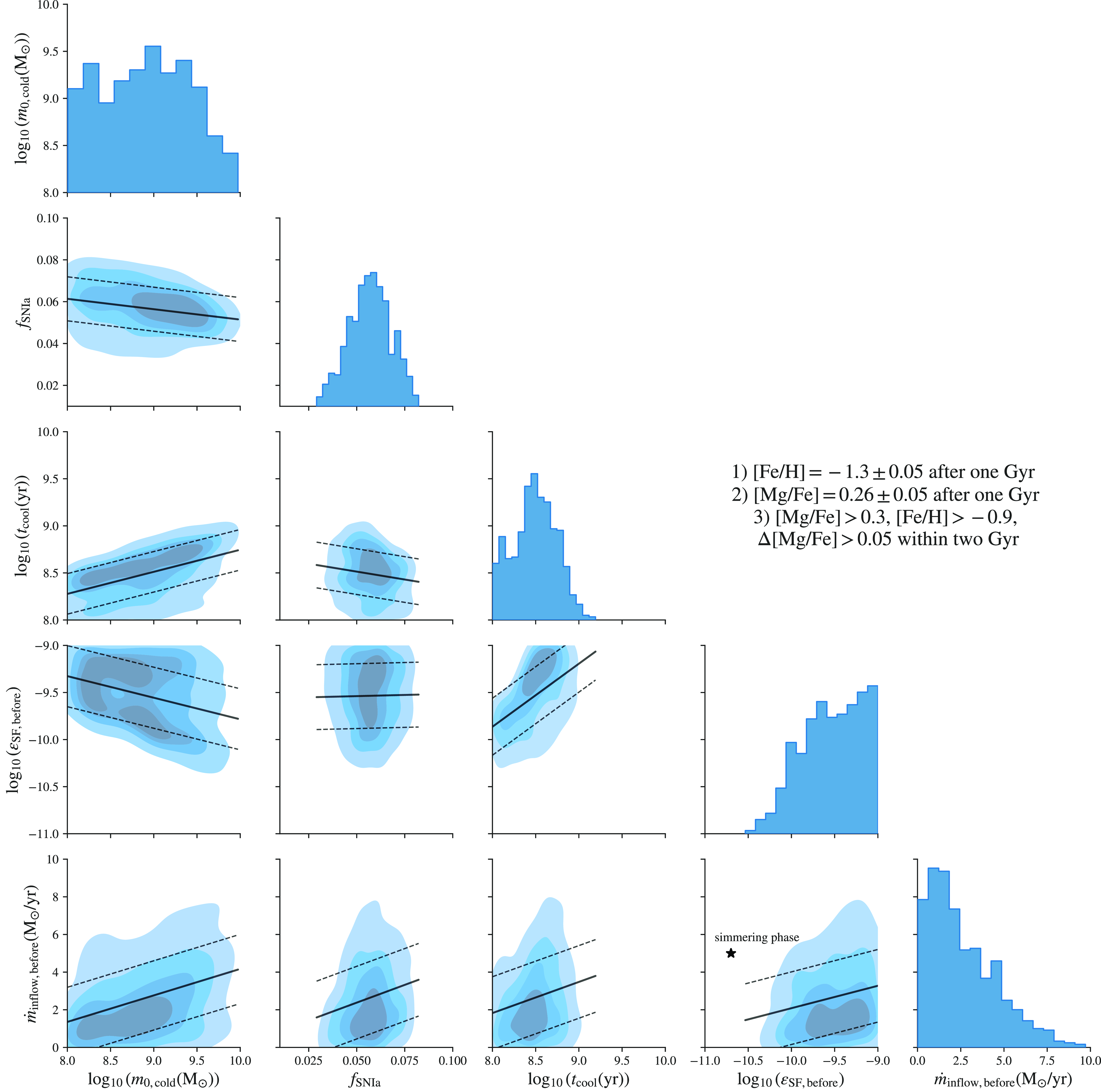
Figure 7. The distribution of parameter values of the models that reach [Fe/H] = $-1.3 \pm 0.05$
and [Mg/Fe]
$-1.3 \pm 0.05$
and [Mg/Fe] $= 0.26 \pm 0.05$
after one Gyr as well as [Mg/Fe]
$= 0.26 \pm 0.05$
after one Gyr as well as [Mg/Fe] $> 0.3$
, [Fe/H]
$> 0.3$
, [Fe/H] $> -0.9$
, and
$> -0.9$
, and $\Delta$
[Mg/Fe]
$\Delta$
[Mg/Fe] $> 0.05$
within two Gyr in the same style as Figs. 5 and 6. The distribution of tracks generated with these parameter values in [Fe/H]-[Mg/Fe] is shown in the bottom panel of Fig. 4.
$> 0.05$
within two Gyr in the same style as Figs. 5 and 6. The distribution of tracks generated with these parameter values in [Fe/H]-[Mg/Fe] is shown in the bottom panel of Fig. 4.
3.3. The rise of [
$\alpha$
/Fe] requires a small existing gas reservoir

Finally, we will examine the parameter distributions of the models that not only reached the [Fe/H]-[ $\alpha$
/Fe]-knee in the first phase but also managed to raise [
$\alpha$
/Fe]-knee in the first phase but also managed to raise [ $\alpha$
/Fe] matching the observations during the second phase. Models whose parameter distributions are displayed in blue in Fig. 7 are required to satisfy all three criteria to complete the [
$\alpha$
/Fe] matching the observations during the second phase. Models whose parameter distributions are displayed in blue in Fig. 7 are required to satisfy all three criteria to complete the [ $\alpha$
/Fe]-reversal. We largely identify the same trends we saw in Figs. 5 and 6, with some exceptions. The relationships in the contours of the parameter distributions as a result of the design of our models still hold, but the joint distributions are refined to a much smaller region in the parameter space.
$\alpha$
/Fe]-reversal. We largely identify the same trends we saw in Figs. 5 and 6, with some exceptions. The relationships in the contours of the parameter distributions as a result of the design of our models still hold, but the joint distributions are refined to a much smaller region in the parameter space.
The most distinguishing feature among models achieving a higher [ $\alpha$
/Fe] value during the second phase is their inflow rate preferentially less than 5
$\alpha$
/Fe] value during the second phase is their inflow rate preferentially less than 5 $\mathrm{M}_\odot$
per year during the first phase. The amount of
$\mathrm{M}_\odot$
per year during the first phase. The amount of $\alpha$
elements needed to raise [
$\alpha$
elements needed to raise [ $\alpha$
/Fe] increases as the mass of low-[
$\alpha$
/Fe] increases as the mass of low-[ $\alpha$
/Fe] gas in a model accumulates through inflow during the first phase. There are two sources for the additional
$\alpha$
/Fe] gas in a model accumulates through inflow during the first phase. There are two sources for the additional $\alpha$
elements. The first is to produce it within the galaxy through enhanced star formation. The release time scale of CCSNe which is primarily responsible for the production of
$\alpha$
elements. The first is to produce it within the galaxy through enhanced star formation. The release time scale of CCSNe which is primarily responsible for the production of $\alpha$
elements is the shortest of all nucleosynthesis channels within our model. Thus, we expect an [
$\alpha$
elements is the shortest of all nucleosynthesis channels within our model. Thus, we expect an [ $\alpha$
/Fe]-rise immediately or flattening of [
$\alpha$
/Fe]-rise immediately or flattening of [ $\alpha$
/Fe] after a star formation burst. The second source is through the accretion of high-[
$\alpha$
/Fe] after a star formation burst. The second source is through the accretion of high-[ $\alpha$
/Fe] gas from the circumgalactic medium (CGM) or mergers. The effect on [
$\alpha$
/Fe] gas from the circumgalactic medium (CGM) or mergers. The effect on [ $\alpha$
/Fe] depends on the [
$\alpha$
/Fe] depends on the [ $\alpha$
/Fe] value, the amount of the accreted gas, and the amount and composition of the gas in the galaxy.
$\alpha$
/Fe] value, the amount of the accreted gas, and the amount and composition of the gas in the galaxy.
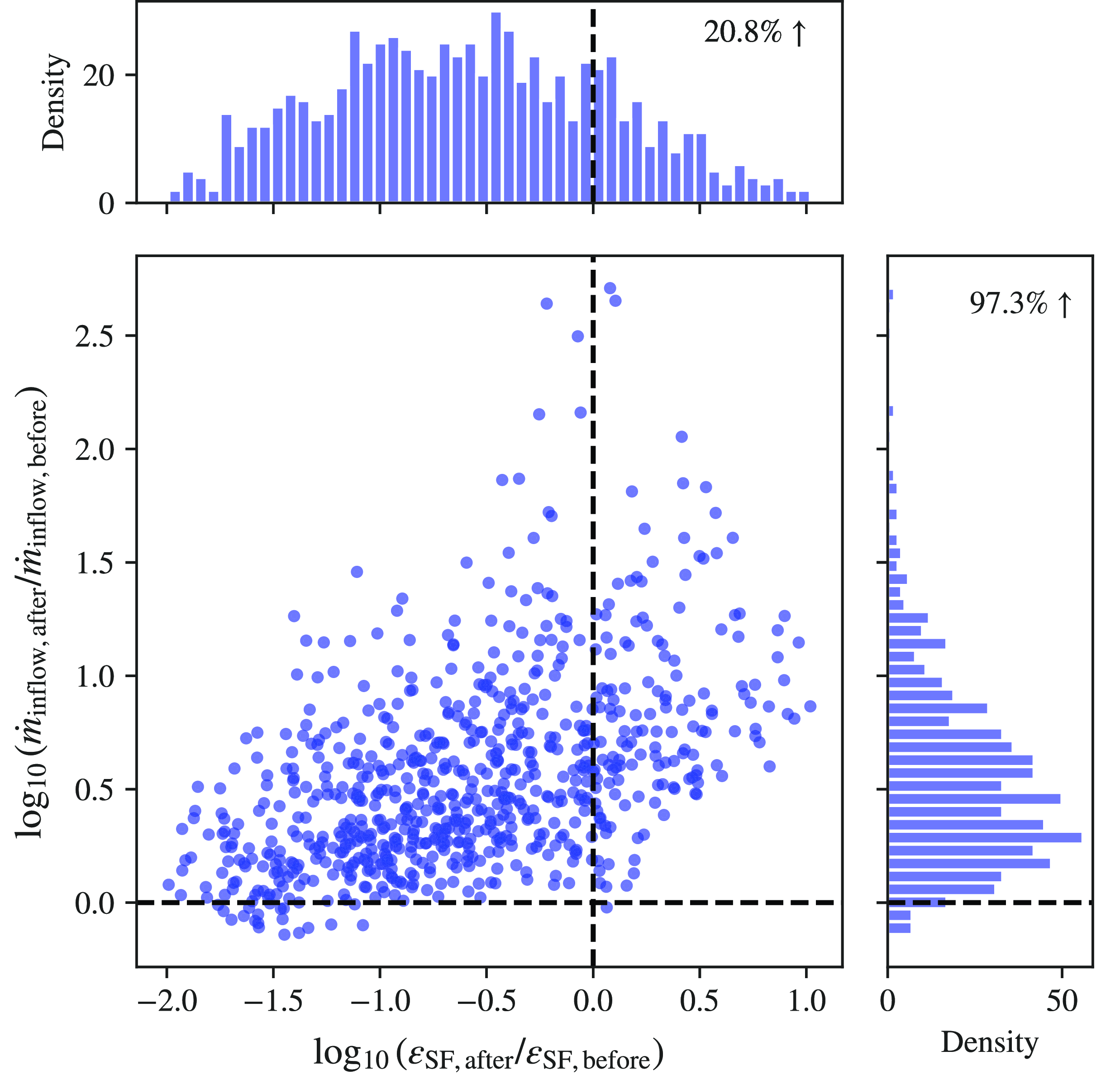
Figure 8. The change in the parameter values of the SFE and inflow rate before vs. after [ $\alpha$
/Fe] reaches the lowest value for models satisfying all three criteria. The dashed line marks where the parameter remains constant. About 20.8% of the models had an increase in the SFE and 97.3% of them experienced an increase in gas inflow rate.
$\alpha$
/Fe] reaches the lowest value for models satisfying all three criteria. The dashed line marks where the parameter remains constant. About 20.8% of the models had an increase in the SFE and 97.3% of them experienced an increase in gas inflow rate.
Examining the change in the SFE and inflow rate reveals that inflow is the primary driver behind the [ $\alpha$
/Fe]-rise. Fig. 8 illustrates the ratios of the SFEs and inflow rates before and after the [Fe/H]-[
$\alpha$
/Fe]-rise. Fig. 8 illustrates the ratios of the SFEs and inflow rates before and after the [Fe/H]-[ $\alpha$
/Fe]-knee for models meeting all three criteria. The ratios are shown in logarithmic scale so zero denotes where the parameter values remain constant. Among the selected models, about 80% had a decrease in their SFE, while over 97% had an increase in their inflow rates. This extreme result could be potentially caused by our choice of [
$\alpha$
/Fe]-knee for models meeting all three criteria. The ratios are shown in logarithmic scale so zero denotes where the parameter values remain constant. Among the selected models, about 80% had a decrease in their SFE, while over 97% had an increase in their inflow rates. This extreme result could be potentially caused by our choice of [ $\alpha$
/Fe] for the inflow gas, the lowering of which could affect these percentages. Nevertheless, we found that models could not reach our [Mg/Fe] target if we lowered [Mg/Fe] in the inflow gas. The changes between SFE and inflow rate appear to be positively correlated. The metallicity of inflow gas during the second phase is fixed around [Fe/H]
$\alpha$
/Fe] for the inflow gas, the lowering of which could affect these percentages. Nevertheless, we found that models could not reach our [Mg/Fe] target if we lowered [Mg/Fe] in the inflow gas. The changes between SFE and inflow rate appear to be positively correlated. The metallicity of inflow gas during the second phase is fixed around [Fe/H] $=-1.3$
. Thus, the more inflow gas a model receives, the more star formation activity needs to happen to reach the metallicity target of [Fe/H]
$=-1.3$
. Thus, the more inflow gas a model receives, the more star formation activity needs to happen to reach the metallicity target of [Fe/H] $=-0.9$
during the second phase. Based on Fig. 8, it is feasible for the SFE in a model to remain constant as [
$=-0.9$
during the second phase. Based on Fig. 8, it is feasible for the SFE in a model to remain constant as [ $\alpha$
/Fe] rises, but the same is unlikely for the inflow rate. Here is the likely scenario from our results so far. The proto-Galaxy started with an initial gas reservoir of moderate mass (
$\alpha$
/Fe] rises, but the same is unlikely for the inflow rate. Here is the likely scenario from our results so far. The proto-Galaxy started with an initial gas reservoir of moderate mass ( $<$
$<$ $10^9$ $\mathrm{M}_\odot$
). It maintained a relatively moderate gas reservoir with little gas inflow as [Fe/H] climbed and [
$\mathrm{M}_\odot$
). It maintained a relatively moderate gas reservoir with little gas inflow as [Fe/H] climbed and [ $\alpha$
/Fe] declined naturally. Through the proto-Galaxy period,
$\alpha$
/Fe] declined naturally. Through the proto-Galaxy period, $f_\textrm{SNIa}$
is around 6%, comparable to today’s value, and the cooling of warm ISM is relatively efficient with
$f_\textrm{SNIa}$
is around 6%, comparable to today’s value, and the cooling of warm ISM is relatively efficient with $t_{\mathrm{cool}} = 10^{8.5}$
yr. A relatively large amount of accreted gas compared to the existing gas reservoir joined the proto-Galaxy around [Fe/H]
$t_{\mathrm{cool}} = 10^{8.5}$
yr. A relatively large amount of accreted gas compared to the existing gas reservoir joined the proto-Galaxy around [Fe/H] $= -1.3$
, increasing the gas inflow rate several times and causing [
$= -1.3$
, increasing the gas inflow rate several times and causing [ $\alpha$
/Fe] to rise.
$\alpha$
/Fe] to rise.
4. Discussion
The purpose of this work is to identify the parameter combinations that will cause [ $\alpha$
/Fe] to rise in the [Fe/H]-[
$\alpha$
/Fe] to rise in the [Fe/H]-[ $\alpha$
/Fe]-plane in the proto-Galaxy from a galactic chemical evolution model and infer the physical condition of the Milky Way before the formation of the disk. We are primarily dealing with two major nucleosynthesis channels in the [Fe/H]-[
$\alpha$
/Fe]-plane in the proto-Galaxy from a galactic chemical evolution model and infer the physical condition of the Milky Way before the formation of the disk. We are primarily dealing with two major nucleosynthesis channels in the [Fe/H]-[ $\alpha$
/Fe]-plane: CCSNe and SNe Ia. Since CCSNe are the primary production site of
$\alpha$
/Fe]-plane: CCSNe and SNe Ia. Since CCSNe are the primary production site of $\alpha$
elements, one way of rising [
$\alpha$
elements, one way of rising [ $\alpha$
/Fe] is through enhanced star formation activity. Another way is to introduce additional
$\alpha$
/Fe] is through enhanced star formation activity. Another way is to introduce additional $\alpha$
elements through gas accretion.
$\alpha$
elements through gas accretion.
There are two channels to boost star formation in the model, which correspond to two scenarios of what could have happened when the disk formed in the Milky Way. The first channel is to increase the SFE. Although the heightened SFE would cause an initial star formation burst, an extended period of star formation would require a sustained stream of gas supply. Otherwise, the existing gas reservoir risks being depleted and the galaxy quenches. Thus, the first scenario entails a high inflow rate of fresh gas to either build up a large gas reservoir before disk formation or to accompany an elevated SFE as soon as the disk forms. The second channel is to introduce additional inflow capable of rapidly cooling to expand the gas reservoir and make more gas available for star formation. However, this requires the existing reservoir to be limited in mass, or the new inflow rate becomes unrealistically large. The ingredients for these two channels are organised in the flowchart in Fig. 1. Due to the uncertainty in the chemical composition of the inflowing gas, it is also possible to introduce additional $\alpha$
elements directly into our Galaxy. We experimented by running our model 300 000 times with randomly generated parameters, two of which, the SFE and inflow rate, were allowed to change after one Gyr of runtime was reached. The results highlight the important role that inflow could have played during the earliest epoch of our Galaxy.
$\alpha$
elements directly into our Galaxy. We experimented by running our model 300 000 times with randomly generated parameters, two of which, the SFE and inflow rate, were allowed to change after one Gyr of runtime was reached. The results highlight the important role that inflow could have played during the earliest epoch of our Galaxy.
We now revisit the two feasible scenarios from our flowchart in Fig. 1. The reversal in the trend of [ $\alpha$
/Fe] requires at least one of two parameters, the SFE and inflow rate, to increase. According to the ‘simmering’ phase, the inflow rate remained high during the entire proto-galaxy phase to build up a sufficiently large gas reservoir. The large increase in the SFE triggered a star formation burst to raise [
$\alpha$
/Fe] requires at least one of two parameters, the SFE and inflow rate, to increase. According to the ‘simmering’ phase, the inflow rate remained high during the entire proto-galaxy phase to build up a sufficiently large gas reservoir. The large increase in the SFE triggered a star formation burst to raise [ $\alpha$
/Fe]. About twenty per cent of our models experienced an increase in their SFEs, which could fall under this scenario. As for the other scenario, about eighty per cent of our models experienced increased inflow. The additional
$\alpha$
/Fe]. About twenty per cent of our models experienced an increase in their SFEs, which could fall under this scenario. As for the other scenario, about eighty per cent of our models experienced increased inflow. The additional $\alpha$
elements could have existed in the inflowing gas already and formed within the galaxy from additional cold ISM. The increase in the gas inflow rate has been suggested by the theoretical calculations by by Rix et al. (Reference Rix2022) as an explanation for the changing slope in the stellar density distribution of [Fe/H] (see their Section 3.2).
$\alpha$
elements could have existed in the inflowing gas already and formed within the galaxy from additional cold ISM. The increase in the gas inflow rate has been suggested by the theoretical calculations by by Rix et al. (Reference Rix2022) as an explanation for the changing slope in the stellar density distribution of [Fe/H] (see their Section 3.2).
The designs of GCE models could affect the details of the parameters. Because the rate and the composition of inflow in Conroy et al. (Reference Conroy2022) were fixed, inflow can only play a limited role in influencing [ $\alpha$
/Fe], in contrast to the design of our model. Their model uses an analytic return function to determine the amount of metals released from stellar bins formed in previous time steps, which most likely makes the recycling of metals more efficient than our model. Thus, they were forced to adopt a low SFE to prevent [Fe/H] from evolving too rapidly. In comparison, our model tracks the stellar lifetimes of stellar bins and uses a warm ISM component to capture newly produced nucleosynthesis yields which are released gradually over time. As a result, our models preferentially adopt high SFEs so that [Fe/H] could reach our target values. One design that requires further justification is the source of high-[
$\alpha$
/Fe], in contrast to the design of our model. Their model uses an analytic return function to determine the amount of metals released from stellar bins formed in previous time steps, which most likely makes the recycling of metals more efficient than our model. Thus, they were forced to adopt a low SFE to prevent [Fe/H] from evolving too rapidly. In comparison, our model tracks the stellar lifetimes of stellar bins and uses a warm ISM component to capture newly produced nucleosynthesis yields which are released gradually over time. As a result, our models preferentially adopt high SFEs so that [Fe/H] could reach our target values. One design that requires further justification is the source of high-[ $\alpha$
/Fe] gas. Accreted structures are typically less massive than the main progenitor and thus tend to have lower [Fe/H] and higher [
$\alpha$
/Fe] gas. Accreted structures are typically less massive than the main progenitor and thus tend to have lower [Fe/H] and higher [ $\alpha$
/Fe]. Metal-poor inflow gas would contain less
$\alpha$
/Fe]. Metal-poor inflow gas would contain less $\alpha$
-elements needed to raise [
$\alpha$
-elements needed to raise [ $\alpha$
/Fe] and force more
$\alpha$
/Fe] and force more $\alpha$
-elements to be produced through CCSNe in the model. It is also possible that a change in the gas cooling mode allows warm ISM with high [
$\alpha$
-elements to be produced through CCSNe in the model. It is also possible that a change in the gas cooling mode allows warm ISM with high [ $\alpha$
/Fe] and similar [Fe/H] in the model to rapidly cool and fuel the formation of high-[
$\alpha$
/Fe] and similar [Fe/H] in the model to rapidly cool and fuel the formation of high-[ $\alpha$
/Fe] stars.
$\alpha$
/Fe] stars.
One key ingredient with high uncertainty in the GCE model is the nucleosynthesis yields. Comparing Figs. 2 and 4, we can see that [Mg/Fe] in our models is higher than observed in H3 at low metallicities due to the high [ $\alpha$
/Fe]-ceiling in our CCSN yields. More SNe Ia is needed to lower [
$\alpha$
/Fe]-ceiling in our CCSN yields. More SNe Ia is needed to lower [ $\alpha$
/Fe] in our models and thus
$\alpha$
/Fe] in our models and thus $f_\textrm{SNIa}$
is likely over-estimated. Andrews et al. (Reference Andrews, Weinberg, Schönrich and Johnson2017) tested different yield sets which all produced similar trends in [Fe/H]-[
$f_\textrm{SNIa}$
is likely over-estimated. Andrews et al. (Reference Andrews, Weinberg, Schönrich and Johnson2017) tested different yield sets which all produced similar trends in [Fe/H]-[ $\alpha$
/Fe] after [Fe/H] exceeds
$\alpha$
/Fe] after [Fe/H] exceeds $-1.8$
(see their Figure 9). Thus, the choice of specific yields should not alter our results, as our work is limited to the study of [Fe/H] and [Mg/Fe] beyond the very metal-poor regime. The [
$-1.8$
(see their Figure 9). Thus, the choice of specific yields should not alter our results, as our work is limited to the study of [Fe/H] and [Mg/Fe] beyond the very metal-poor regime. The [ $\alpha$
/Fe]-rise could also be seen in other
$\alpha$
/Fe]-rise could also be seen in other $\alpha$
-elements, such as [Al/Fe] in Belokurov & Kravtsov (Reference Belokurov and Kravtsov2022). Different yields could result in significantly different physical conditions for these elements. Nevertheless, adjusting the efficiency of physical processes could mitigate the changes in the yield of specific elements (Weinberg et al. Reference Weinberg, Griffith, Johnson and Thompson2023). A different yield set might shift the quantitative trends in our results, but it would not alter our conclusion due to a high degree of freedom in the parameter choice in our design.
$\alpha$
-elements, such as [Al/Fe] in Belokurov & Kravtsov (Reference Belokurov and Kravtsov2022). Different yields could result in significantly different physical conditions for these elements. Nevertheless, adjusting the efficiency of physical processes could mitigate the changes in the yield of specific elements (Weinberg et al. Reference Weinberg, Griffith, Johnson and Thompson2023). A different yield set might shift the quantitative trends in our results, but it would not alter our conclusion due to a high degree of freedom in the parameter choice in our design.
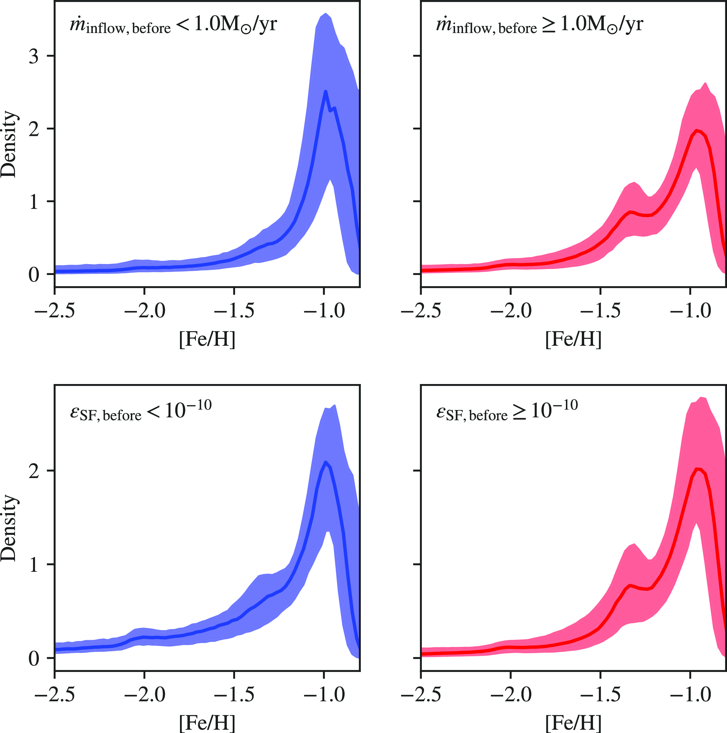
Figure 9. Stellar density of [Fe/H] for models exhibiting an increase in [ $\alpha$
/Fe] satisfying all three criteria, separated by their inflow rates and SFEs during the first stage.
$\alpha$
/Fe] satisfying all three criteria, separated by their inflow rates and SFEs during the first stage.
4.1. Further constraining parameters of proto Milky Way
We adopted a limited time frame (two Gyr) and specific criteria to reproduce the [ $\alpha$
/Fe]-rise in our GCE model in this work, i.e. [Fe/H]
$\alpha$
/Fe]-rise in our GCE model in this work, i.e. [Fe/H] $ = -1.3 \pm 0.05$
, [Mg/Fe]
$ = -1.3 \pm 0.05$
, [Mg/Fe] $ = 0.26 \pm 0.05$
after one Gyr and [Mg/Fe]
$ = 0.26 \pm 0.05$
after one Gyr and [Mg/Fe] $> 0.3$
as well as [Fe/H] > -0.9 within two Gyr. The time frame was chosen to accommodate the possibility of a twelve-Gyr-old thick disk. The three elemental ratios were chosen to constrain parameter confounding to more clearly identify the parameter combinations that would produce the [
$> 0.3$
as well as [Fe/H] > -0.9 within two Gyr. The time frame was chosen to accommodate the possibility of a twelve-Gyr-old thick disk. The three elemental ratios were chosen to constrain parameter confounding to more clearly identify the parameter combinations that would produce the [ $\alpha$
/Fe] trend we approximated from observations. Changing the key abundance ratios in the criteria or allowing larger margins could shift the parameter distributions, but it will not invalidate the qualitative trends we observed in Figs. 6 and 7. However, as the precision of the abundance measurements improves or the age estimates for the stars in question become available, we expect to come up with a quantitative approximation of the track rather than three abundance ratios. We can then further fine-tune our parameter choices by controlling the rate of chemical evolution in the model.
$\alpha$
/Fe] trend we approximated from observations. Changing the key abundance ratios in the criteria or allowing larger margins could shift the parameter distributions, but it will not invalidate the qualitative trends we observed in Figs. 6 and 7. However, as the precision of the abundance measurements improves or the age estimates for the stars in question become available, we expect to come up with a quantitative approximation of the track rather than three abundance ratios. We can then further fine-tune our parameter choices by controlling the rate of chemical evolution in the model.
There are other properties we can examine, besides the chemical evolutionary track. Although models with different SFEs can achieve the same key abundance ratios, their stellar chemical distribution and global properties are vastly different. Fig. 9 shows the metallicity distribution function (MDF) of the models satisfying all three criteria for the [ $\alpha$
/Fe]-rise divided into two groups based on their initial inflow rate (top) and SFE (bottom). Models with relatively high initial inflow rates and SFEs show a prominent peak at [Fe/H]
$\alpha$
/Fe]-rise divided into two groups based on their initial inflow rate (top) and SFE (bottom). Models with relatively high initial inflow rates and SFEs show a prominent peak at [Fe/H] $=-1.3$
when the second phase commences. Therefore, it is feasible to distinguish the two scenarios in Fig. 1 from the observed MDF, given we have a large sample of metal-poor stars. The scenario with a high initial SFE predicts that there should be at least one peak around [Fe/H] = -1.3 in the MDF, while the absence of such features would favour the low-SFE scenario. Fig. 10 shows the evolution of the global properties of the same models in Fig. 9 over time, colour-coded again by the initial SFE. Specifically, we show the mass of cold ISM, warm ISM, and stars as well as the mass ratio between stars and cold gas over running time. Except for the stellar mass and warm gas panel, the other two panels show strong correlations of the properties with the SFEs. As a sufficient number of metal-poor stars are observed in the future to accurately map the MDF and ADF at low metallicity and high [
$=-1.3$
when the second phase commences. Therefore, it is feasible to distinguish the two scenarios in Fig. 1 from the observed MDF, given we have a large sample of metal-poor stars. The scenario with a high initial SFE predicts that there should be at least one peak around [Fe/H] = -1.3 in the MDF, while the absence of such features would favour the low-SFE scenario. Fig. 10 shows the evolution of the global properties of the same models in Fig. 9 over time, colour-coded again by the initial SFE. Specifically, we show the mass of cold ISM, warm ISM, and stars as well as the mass ratio between stars and cold gas over running time. Except for the stellar mass and warm gas panel, the other two panels show strong correlations of the properties with the SFEs. As a sufficient number of metal-poor stars are observed in the future to accurately map the MDF and ADF at low metallicity and high [ $\alpha$
/Fe], we can constrain the SFE and other parameters more precisely based on the detailed chemical distribution of the in situ population in the early Milky Way. Alternatively, we could examine the global properties of the Milky Way analogs in simulations to narrow down the parameters. We will subsequently discuss the complexities of our findings in the context of prior relevant studies.
$\alpha$
/Fe], we can constrain the SFE and other parameters more precisely based on the detailed chemical distribution of the in situ population in the early Milky Way. Alternatively, we could examine the global properties of the Milky Way analogs in simulations to narrow down the parameters. We will subsequently discuss the complexities of our findings in the context of prior relevant studies.
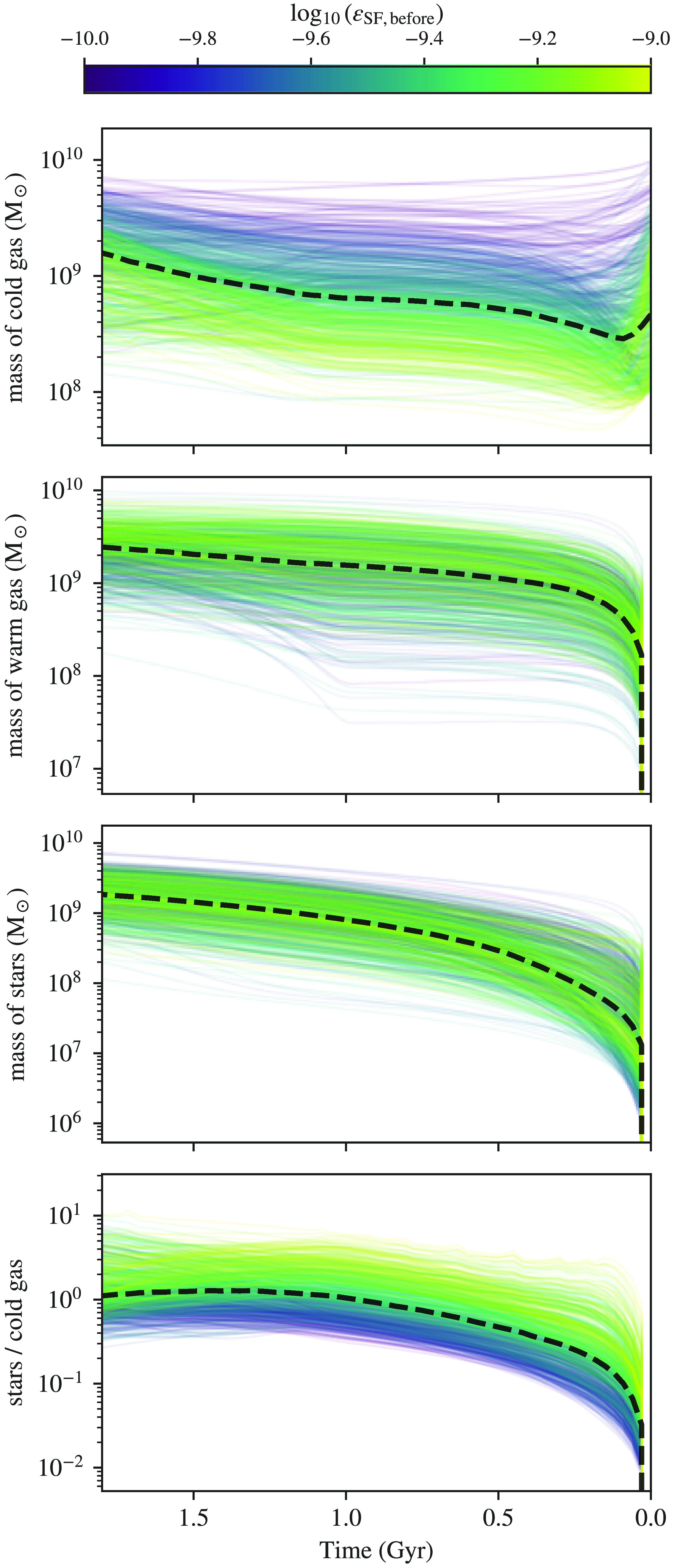
Figure 10. The masses of baryonic components of the models that satisfy all three criteria during the running time. The panels from top to bottom show the evolution of the total cold gas mass, warm gas mass, stellar mass, and the ratio between cold gas and stellar mass.
4.2. The inflow that fueled the Milky Way
There are two physically distinct regimes of gas accretion onto galaxies: a ‘cold’ filamentary mode in which warm gas ( $<$
$<$ $10^{5}$
K) accretes along filaments that can penetrate to the inner regions of halos and a ‘hot’ flow mode wherein hot diffuse gas in extended halos cools over time (Kereš et al. Reference Kereš, Katz, Weinberg and Davé2005, Reference Kereš, Katz, Davé, Fardal and Wein-berg2009) The cold accretion mode is more common in smaller galaxies and the hot mode is more common in massive galaxies. The important role of gas accretion has been established by cosmological simulations but the properties of accreted gas have been difficult to quantify because the baryon cycle is a complex process that involves the continuous interplay of gas inflow, outflow, and star formation (Dekel et al. 2009; van de Voort et al. Reference van de Voort, Schaye, Booth, Haas and Vecchia2011; Lagos et al. Reference Lagos, Baugh, Zwaan, Lacey, Gonzalez-Perez, Power, Swinbank and van Kampen2014; Nelson et al. Reference Nelson, Genel, Vogelsberger, Springel, Si-jacki, Torrey and Hernquist2015; Correa et al. Reference Correa, Schaye, van de Voort, Duffy and Wyithe2018; Mitchell et al. Reference Mitchell, Schaye, Bower and Crain2020; Wright et al. 2020). The prototypes of Milky Way analogs in cosmological simulations at high redshift experience rapid gas accretion through cold streams with large angular momentum which is subsequently transferred to the existing halo, contributing to the increased spin of these galaxies (Stewart et al. Reference Stewart, Kaufmann, Bullock, Barton, Maller, Diemand and Wadsley2011; Sales et al. Reference Sales, Navarro, Theuns, Schaye, White, Frenk, Crain and Vecchia2012; Danovich et al. Reference Danovich, Dekel, Hahn, Ceverino and Primack2015). However, before the filaments with different directions become aligned and settle into disks, Milky Way prototypes take the shape of spheroids characterized by an extended profile and violent kinematics (Rosdahl & Blaizot Reference Rosdahl and Blaizot2012; Stewart et al. Reference Stewart, Brooks, Bullock, Maller, Diemand, Wadsley and Moustakas2013; Obreja et al. Reference Obreja, Domnguez-Tenreiro, Brook, Martínez-Serrano, Doménech-Moral, Serna, Mollá and Stinson2013, Reference Obreja2019; Bird et al. Reference Bird, Kazantzidis, Weinberg, Guedes, Callegari, Mayer and Madau2013, Reference Bird, Loebman, Weinberg, Brooks, Quinn and Christensen2021; Meng, Gnedin, & Li Reference Meng, Gnedin and Li2019). As these galaxies accrete more gas, they become massive enough to support a hot halo which subsequently triggers the transition from ‘cold’ mode accretion to ‘hot’ mode accretion, accompanied by the formation of a gaseous disk (Dekel et al. Reference Dekel, Ginzburg, Jiang, Freundlich, Lapiner, Ceverino and Primack2020; Stern et al. Reference Stern2021; Hafen et al. Reference Hafen2022; Gurvich et al. Reference Gurvich2023). Therefore, the [
$10^{5}$
K) accretes along filaments that can penetrate to the inner regions of halos and a ‘hot’ flow mode wherein hot diffuse gas in extended halos cools over time (Kereš et al. Reference Kereš, Katz, Weinberg and Davé2005, Reference Kereš, Katz, Davé, Fardal and Wein-berg2009) The cold accretion mode is more common in smaller galaxies and the hot mode is more common in massive galaxies. The important role of gas accretion has been established by cosmological simulations but the properties of accreted gas have been difficult to quantify because the baryon cycle is a complex process that involves the continuous interplay of gas inflow, outflow, and star formation (Dekel et al. 2009; van de Voort et al. Reference van de Voort, Schaye, Booth, Haas and Vecchia2011; Lagos et al. Reference Lagos, Baugh, Zwaan, Lacey, Gonzalez-Perez, Power, Swinbank and van Kampen2014; Nelson et al. Reference Nelson, Genel, Vogelsberger, Springel, Si-jacki, Torrey and Hernquist2015; Correa et al. Reference Correa, Schaye, van de Voort, Duffy and Wyithe2018; Mitchell et al. Reference Mitchell, Schaye, Bower and Crain2020; Wright et al. 2020). The prototypes of Milky Way analogs in cosmological simulations at high redshift experience rapid gas accretion through cold streams with large angular momentum which is subsequently transferred to the existing halo, contributing to the increased spin of these galaxies (Stewart et al. Reference Stewart, Kaufmann, Bullock, Barton, Maller, Diemand and Wadsley2011; Sales et al. Reference Sales, Navarro, Theuns, Schaye, White, Frenk, Crain and Vecchia2012; Danovich et al. Reference Danovich, Dekel, Hahn, Ceverino and Primack2015). However, before the filaments with different directions become aligned and settle into disks, Milky Way prototypes take the shape of spheroids characterized by an extended profile and violent kinematics (Rosdahl & Blaizot Reference Rosdahl and Blaizot2012; Stewart et al. Reference Stewart, Brooks, Bullock, Maller, Diemand, Wadsley and Moustakas2013; Obreja et al. Reference Obreja, Domnguez-Tenreiro, Brook, Martínez-Serrano, Doménech-Moral, Serna, Mollá and Stinson2013, Reference Obreja2019; Bird et al. Reference Bird, Kazantzidis, Weinberg, Guedes, Callegari, Mayer and Madau2013, Reference Bird, Loebman, Weinberg, Brooks, Quinn and Christensen2021; Meng, Gnedin, & Li Reference Meng, Gnedin and Li2019). As these galaxies accrete more gas, they become massive enough to support a hot halo which subsequently triggers the transition from ‘cold’ mode accretion to ‘hot’ mode accretion, accompanied by the formation of a gaseous disk (Dekel et al. Reference Dekel, Ginzburg, Jiang, Freundlich, Lapiner, Ceverino and Primack2020; Stern et al. Reference Stern2021; Hafen et al. Reference Hafen2022; Gurvich et al. Reference Gurvich2023). Therefore, the [ $\alpha$
/Fe]-rise could be a chemical signature for the ‘cold’ accretion that happened during the proto-Galaxy.
$\alpha$
/Fe]-rise could be a chemical signature for the ‘cold’ accretion that happened during the proto-Galaxy.
Our work is closely connected to a series of recent works on the pre-disk Milky Way. Belokurov & Kravtsov (Reference Belokurov and Kravtsov2022) found chemical and dynamical signatures for the ‘cold’ accretion among a large number of stars before the coherent disk in the Galaxy formed and named this population Aurora. The features of this population are consistent with the scenario under which stars form in cold filaments that are rapidly accreted onto the Galaxy. The stars have a large scatter in elemental abundances which could be caused by the diverse conditions under which nucleosynthesis took place. Its spheroidal spatial distribution and isotropic velocity ellipsoid are expected from simulated galaxies that went through the chaotic phase of evolution. Additionally, these stars showed a strong positive correlation between metallicity and tangential velocity, which is a signature of the filaments transferring their high angular momentum to our Galaxy. Conroy et al. (Reference Conroy2022) extended the metallicity coverage of this population, especially towards the metal-poor end, and presented us a more complete picture of the [ $\alpha$
/Fe]-rise. The dynamical aspect of these works is corroborated by Yu et al. (Reference Yu2023) that showed that the orbits of in situ stars are closely related to their respective formation epoch from simulated Milky Way-mass galaxies in FIRE. Our accretion scenario suggests that the cold accretion should take time to ramp up in the proto-Galaxy.
$\alpha$
/Fe]-rise. The dynamical aspect of these works is corroborated by Yu et al. (Reference Yu2023) that showed that the orbits of in situ stars are closely related to their respective formation epoch from simulated Milky Way-mass galaxies in FIRE. Our accretion scenario suggests that the cold accretion should take time to ramp up in the proto-Galaxy.
Our results offer additional evidence from the perspective of chemical evolution that the brief [ $\alpha$
/Fe]-rise in the [Fe/H]-[
$\alpha$
/Fe]-rise in the [Fe/H]-[ $\alpha$
/Fe]-plane is a signature of massive inflow that ended the prototype phase of the Milky Way and initiated the physical process through which the disk later formed. Although our GCE model does not simulate the dynamical features of our Galaxy during its earliest epoch, it is flexible with a wide selection of parameters governing the chemical evolution to explore the conditions behind the [
$\alpha$
/Fe]-plane is a signature of massive inflow that ended the prototype phase of the Milky Way and initiated the physical process through which the disk later formed. Although our GCE model does not simulate the dynamical features of our Galaxy during its earliest epoch, it is flexible with a wide selection of parameters governing the chemical evolution to explore the conditions behind the [ $\alpha$
/Fe]-rise. Although it is reasonable to expect the SFE to rise to facilitate enhanced star formation, our model showed that inflow must be suppressed until the rise of [
$\alpha$
/Fe]-rise. Although it is reasonable to expect the SFE to rise to facilitate enhanced star formation, our model showed that inflow must be suppressed until the rise of [ $\alpha$
/Fe], while the SFE plays a secondary role when high-[
$\alpha$
/Fe], while the SFE plays a secondary role when high-[ $\alpha$
/Fe] inflow is available. This scenario agrees with the cold mode accretion that fueled the formation of the early Milky Way suggested by Belokurov & Kravtsov (Reference Belokurov and Kravtsov2022). Nevertheless, the SFE could play a more important role if we lower the [
$\alpha$
/Fe] inflow is available. This scenario agrees with the cold mode accretion that fueled the formation of the early Milky Way suggested by Belokurov & Kravtsov (Reference Belokurov and Kravtsov2022). Nevertheless, the SFE could play a more important role if we lower the [ $\alpha$
/Fe] value of inflow. Rix et al. (Reference Rix2022) estimated their in situ metal-poor sample to have a stellar mass
$\alpha$
/Fe] value of inflow. Rix et al. (Reference Rix2022) estimated their in situ metal-poor sample to have a stellar mass $\mathrm{M_*} > 10^{8}$ $\mathrm{M}_\odot$
which also agrees with the median stellar mass of the proto-Milky Way from our model (see Fig. 10).
$\mathrm{M}_\odot$
which also agrees with the median stellar mass of the proto-Milky Way from our model (see Fig. 10).
4.3. Contamination from accreted stellar structures
The stellar sample may exhibit the observed [ $\alpha$
/Fe]-rise is contaminated by accreted stellar structures. Distinguishing in situ and accreted stars in the halo of the Milky Way is primarily done through the analysis of their kinematic and chemical properties, but it is unclear to what extent the properties are related to the birth origin of stars. The kinematic properties of stars, such as their orbits and angular momentum characteristics, can provide insights into their origin and formation history. Accreted stars in the halo are typically associated with tidal debris from disrupted satellite galaxies, such as Sagittarius and Gaia-Sausage-Enceladus, and have highly inclined or eccentric orbits (Belokurov et al. Reference Belokurov, Erkal, Evans, Koposov and Deason2018; Helmi et al. Reference Helmi, Babusiaux, Koppelman, Massari, Veljanoski and Brown2018). The presence of disrupted star clusters in the stellar halo is also indicative of an accreted component (Malhan, Ibata, & Martin Reference Malhan, Ibata and Martin2018; Shipp et al. Reference Shipp2018; Bonaca et al. Reference Bonaca2021). Nevertheless, even among in situ stars in simulated Milky Way analogs, there is a wide range of dynamical features (Yu et al. Reference Yu2023). Elemental abundances can also be used to distinguish in situ and accreted stars in the halo. The distinct abundance patterns of accreted stars in the [Fe/H]-[
$\alpha$
/Fe]-rise is contaminated by accreted stellar structures. Distinguishing in situ and accreted stars in the halo of the Milky Way is primarily done through the analysis of their kinematic and chemical properties, but it is unclear to what extent the properties are related to the birth origin of stars. The kinematic properties of stars, such as their orbits and angular momentum characteristics, can provide insights into their origin and formation history. Accreted stars in the halo are typically associated with tidal debris from disrupted satellite galaxies, such as Sagittarius and Gaia-Sausage-Enceladus, and have highly inclined or eccentric orbits (Belokurov et al. Reference Belokurov, Erkal, Evans, Koposov and Deason2018; Helmi et al. Reference Helmi, Babusiaux, Koppelman, Massari, Veljanoski and Brown2018). The presence of disrupted star clusters in the stellar halo is also indicative of an accreted component (Malhan, Ibata, & Martin Reference Malhan, Ibata and Martin2018; Shipp et al. Reference Shipp2018; Bonaca et al. Reference Bonaca2021). Nevertheless, even among in situ stars in simulated Milky Way analogs, there is a wide range of dynamical features (Yu et al. Reference Yu2023). Elemental abundances can also be used to distinguish in situ and accreted stars in the halo. The distinct abundance patterns of accreted stars in the [Fe/H]-[ $\alpha$
/Fe] or [Mg/Mn]-[Al/Fe] plane suggest an accreted origin, indicating that their birth material was enriched in a lower mass potential well, such as a satellite galaxy (Hawkins et al. Reference Hawkins, Jofré, Masseron and Gilmore2015; Lee et al. Reference Lee, Johnston, Sen and Jessop2015; Belokurov et al. Reference Belokurov, Sanders, Fattahi, Smith, Deason, Wyn Evans and Grand2019; Feuillet et al. Reference Feuillet, Sahlholdt, Feltzing and Casagrande2021; Horta et al. Reference Horta2023b). The question of distinguishing the birth origin of stars is possibly moot during the proto-Galaxy phase. El-Badry et al. (Reference El-Badry2018) studied the distribution of ancient stars in simulated Milky Way analogs in detail and found that most of the oldest stars are accreted through hierarchical assembly. At
$\alpha$
/Fe] or [Mg/Mn]-[Al/Fe] plane suggest an accreted origin, indicating that their birth material was enriched in a lower mass potential well, such as a satellite galaxy (Hawkins et al. Reference Hawkins, Jofré, Masseron and Gilmore2015; Lee et al. Reference Lee, Johnston, Sen and Jessop2015; Belokurov et al. Reference Belokurov, Sanders, Fattahi, Smith, Deason, Wyn Evans and Grand2019; Feuillet et al. Reference Feuillet, Sahlholdt, Feltzing and Casagrande2021; Horta et al. Reference Horta2023b). The question of distinguishing the birth origin of stars is possibly moot during the proto-Galaxy phase. El-Badry et al. (Reference El-Badry2018) studied the distribution of ancient stars in simulated Milky Way analogs in detail and found that most of the oldest stars are accreted through hierarchical assembly. At $z = 5$
(
$z = 5$
( $\sim$ $1.1$
Gyr after the Big Bang), the main progenitors of the Milky Way analogs contained only half of the old stars in stellar mass or less. Horta et al. (Reference Horta2023a) found that it is common for Milky Way analogs to have multiple progenitors with one or two dominant systems in simulations. If the observed [
$1.1$
Gyr after the Big Bang), the main progenitors of the Milky Way analogs contained only half of the old stars in stellar mass or less. Horta et al. (Reference Horta2023a) found that it is common for Milky Way analogs to have multiple progenitors with one or two dominant systems in simulations. If the observed [ $\alpha$
/Fe]-rise were manifested in one or multiple accreted structures, they likely represented a significant portion of the stellar mass of the proto-Galaxy.
$\alpha$
/Fe]-rise were manifested in one or multiple accreted structures, they likely represented a significant portion of the stellar mass of the proto-Galaxy.
4.4. Implications on future GCE studies of the Milky Way disk
One of the challenges to studying the Milky Way disk with GCE models is setting the initial conditions when the disk first formed. The standard approach consists of initializing a GCE model with a reservoir of pristine gas and growing the reservoir over time with pristine or very metal-poor ([Fe/H] < -1) inflowing gas. The high initial inflow rate of the exponential form over time is justified from the perspective of chemical evolution because a high SFR is required to form the right amount of high-[ $\alpha$
/Fe] stars in the Milky Way disk (Kubryk Prantzos, & Athanassoula Reference Kubryk, Prantzos and Athanassoula2015; Minchev, Chiappini, & Martig Reference Minchev, Chiappini and Martig2013; Johnson et al. Reference Johnson2021; Chen et al. Reference Chen, Hayden, Sharma, Bland-Hawthorn, Kobayashi and Karakas2023). However, it is difficult to synchronize the evolution of [Fe/H] and [
$\alpha$
/Fe] stars in the Milky Way disk (Kubryk Prantzos, & Athanassoula Reference Kubryk, Prantzos and Athanassoula2015; Minchev, Chiappini, & Martig Reference Minchev, Chiappini and Martig2013; Johnson et al. Reference Johnson2021; Chen et al. Reference Chen, Hayden, Sharma, Bland-Hawthorn, Kobayashi and Karakas2023). However, it is difficult to synchronize the evolution of [Fe/H] and [ $\alpha$
/Fe] with this approach to match the key abundance ratios of the Milky Way disc. It only takes a few hundred Myr to one Gyr for SNe Ia to start impacting [
$\alpha$
/Fe] with this approach to match the key abundance ratios of the Milky Way disc. It only takes a few hundred Myr to one Gyr for SNe Ia to start impacting [ $\alpha$
/Fe], but it takes at least one Gyr for [Fe/H] to reach
$\alpha$
/Fe], but it takes at least one Gyr for [Fe/H] to reach $-1.0$
. For example, only 4.7% of our models reached [Fe/H]
$-1.0$
. For example, only 4.7% of our models reached [Fe/H] $\approx -1.3$
in one Gyr. The mismatch between [Fe/H] and [
$\approx -1.3$
in one Gyr. The mismatch between [Fe/H] and [ $\alpha$
/Fe] leads to contradictory choices on the SFE. We need a high SFE for [Fe/H] to evolve quickly and form enough high-[
$\alpha$
/Fe] leads to contradictory choices on the SFE. We need a high SFE for [Fe/H] to evolve quickly and form enough high-[ $\alpha$
/Fe] stars, but the combination of a high SFE and a high gas inflow rate forms too many metal-poor stars and forces [
$\alpha$
/Fe] stars, but the combination of a high SFE and a high gas inflow rate forms too many metal-poor stars and forces [ $\alpha$
/Fe] to depress before [Fe/H] can reach the target value in our Galaxy. Even if a model can reach the target values for [Fe/H] and [
$\alpha$
/Fe] to depress before [Fe/H] can reach the target value in our Galaxy. Even if a model can reach the target values for [Fe/H] and [ $\alpha$
/Fe], it can rarely sustain high [
$\alpha$
/Fe], it can rarely sustain high [ $\alpha$
/Fe] for a few hundred Myr, while the ages of thick disk stars could range from eight hundred Myr after the Big Bang to about eight Gyr (Xiang & Rix Reference Xiang and Rix2022).
$\alpha$
/Fe] for a few hundred Myr, while the ages of thick disk stars could range from eight hundred Myr after the Big Bang to about eight Gyr (Xiang & Rix Reference Xiang and Rix2022).
The scenario for the proto-Galaxy outlined in our work solves the above issues and allows future GCE studies of the Milky Way disk to set initial conditions in a self-consistent approach. The inflow is initially suppressed in the model, allowing [Fe/H] to evolve quickly under a high-SFE regime without forming too many metal-poor stars. We had a fixed time stamp for [Fe/H] to reach around $-1.3$
at one Gyr in our model. In the middle panel of Fig. 10, the median stellar mass of our models is about
$-1.3$
at one Gyr in our model. In the middle panel of Fig. 10, the median stellar mass of our models is about $5 \times 10^8$ $\mathrm{M}_\odot$
. It is unavoidable for [
$\mathrm{M}_\odot$
. It is unavoidable for [ $\alpha$
/Fe] to drop as soon as SNe Ia set off, but we rejuvenate the gas reservoir with a relatively large amount of high-[
$\alpha$
/Fe] to drop as soon as SNe Ia set off, but we rejuvenate the gas reservoir with a relatively large amount of high-[ $\alpha$
/Fe] fresh gas. Since the initial gas reservoir is limited in mass, the large amount of fresh gas leads to a new episode of star formation which helps raise [
$\alpha$
/Fe] fresh gas. Since the initial gas reservoir is limited in mass, the large amount of fresh gas leads to a new episode of star formation which helps raise [ $\alpha$
/Fe] and further elevate [Fe/H]. The massive amount of new stars and introduced high-[
$\alpha$
/Fe] and further elevate [Fe/H]. The massive amount of new stars and introduced high-[ $\alpha$
/Fe] gas temporarily delays the effect of the SNe Ia from the earliest stars and keeps [
$\alpha$
/Fe] gas temporarily delays the effect of the SNe Ia from the earliest stars and keeps [ $\alpha$
/Fe] relatively high long enough to match the large age spread of high-[
$\alpha$
/Fe] relatively high long enough to match the large age spread of high-[ $\alpha$
/Fe] stars.
$\alpha$
/Fe] stars.
5. Conclusion
In this study, we deepened our understanding of the [ $\alpha/\text{Fe}$
]-rise observed in H3 and APOGEE data through a comprehensive investigation using our GCE Model. The main findings are as follows:
$\alpha/\text{Fe}$
]-rise observed in H3 and APOGEE data through a comprehensive investigation using our GCE Model. The main findings are as follows:
-
• The [
$\alpha/\text{Fe}$
]-rise could be principally driven by gas inflow, thus adding a chemical evolution perspective to theories surrounding the Milky Way disk’s spin-up phase. Specifically, the ISM of the proto-Galaxy initially appeared isolated to facilitate a quick rise in [Fe/H] and later underwent rapid gas accretion. -
• When [
$\alpha$
/Fe]-rich inflow is present, the SFE does not play a deterministic role in the [
$\alpha/\text{Fe}$
]-rise, even though in theory the rise in the SFE should facilitate the [
$\alpha/\text{Fe}$
]-rise. The SFEs in our models on average decreased and yet the models still produced the observed [
$\alpha/\text{Fe}$
] rise under certain conditions. -
• Our models suggest that the earliest proto-Galaxy had an initial cold gas reservoir less massive than
$10^9 \text{M}_\odot$
, along with efficient cooling of the warm ISM on a timescale of
$10^{8.5}$
yr. The SFE was comparable to the present-day value, if not higher. Our models also indicate a similar frequency of SNe Ia to the present-day value, which involves around 4% of white dwarfs originating from stars within [3, 8]
$\text{M}_\odot$
.


Our model provides a coherent framework that addresses several key questions in the chemical evolution of the Milky Way
-
• Our model addresses the lack of metal-poor stars by initially suppressing gas inflow, which also allows for rapid evolution of [Fe/H] without dilution from metal-poor gas. The moderate mass of the initial gas reservoir and low gas accretion rate restrict the amount of gas available for star formation, which explains the lack of metal-poor stars in observations.
-
• Our model accommodates the observed plateau in [
$\alpha/\text{Fe}$
] values by introducing a higher inflow rate after the initial phase. This accretion episode initiates heightened star formation activity and allows for a sustained high [
$\alpha/\text{Fe}$
] level three to four Gyr after the Big Bang. This explains why the thick disk’s [
$\alpha/\text{Fe}$
] values plateau at around 0.3 dex, lower than those predicted by CCSNe (
$\sim$
0.4–0.5 dex) -
• By allowing for a rejuvenated gas reservoir with higher inflow rates, our model captures the startup of the disk formation from the perspective of chemical evolution and collaborates existing proposed scenarios for the formation of the thick disk. The accreted gas could provide the angular momentum to support the spinning up of our disk.


Finally, we note that the [ $\alpha/\text{Fe}$
]-rise alone leaves considerable ambiguity in model parameters, leading to some degree of degeneracy. We chose [
$\alpha/\text{Fe}$
]-rise alone leaves considerable ambiguity in model parameters, leading to some degree of degeneracy. We chose [ $\alpha$
/Fe]-rich inflow to facilitate the [
$\alpha$
/Fe]-rich inflow to facilitate the [ $\alpha$
/Fe]-rise, but [
$\alpha$
/Fe]-rise, but [ $\alpha$
/Fe]-poor inflow could place additional emphasis on enhanced SFEs. Our findings suggest that future observations – whether focused on gas mass or the distribution function in [Fe/H] and [
$\alpha$
/Fe]-poor inflow could place additional emphasis on enhanced SFEs. Our findings suggest that future observations – whether focused on gas mass or the distribution function in [Fe/H] and [ $\alpha/\text{Fe}$
] – could significantly improve our understanding of the ancient history of our Galaxy. A magnitude-complete survey of photometric metallicities could provide us with the observed MDF to break the degeneracies among the parameters. Recently available metallicity catalogs derived from the Gaia XP spectra could be ideal candidates for such studies (Andrae, Rix, & Chandra Reference Andrae, Rix and Chandra2023; Zhang, Green, & Rix Reference Zhang, Green and Rix2023). Besides [
$\alpha/\text{Fe}$
] – could significantly improve our understanding of the ancient history of our Galaxy. A magnitude-complete survey of photometric metallicities could provide us with the observed MDF to break the degeneracies among the parameters. Recently available metallicity catalogs derived from the Gaia XP spectra could be ideal candidates for such studies (Andrae, Rix, & Chandra Reference Andrae, Rix and Chandra2023; Zhang, Green, & Rix Reference Zhang, Green and Rix2023). Besides [ $\alpha$
/Fe], other abundance ratios could provide additional insight into the earliest epoch of our Galaxy (Schiavon et al. Reference Schiavon2017; Kisku et al. Reference Kisku2021; Horta et al. Reference Horta2021a; Phillips et al. Reference Phillips2022). In a broader context, the methodology and insights gleaned from this study extend beyond the Milky Way. Similar approaches could be applied to other intriguing galaxies, such as M31 and the Large Magellanic Cloud, the latter of which have also shown fascinating chemical evolution patterns (Nidever et al. Reference Nidever2020). This opens up a wide field for future research. Our work emphasizes the ongoing importance of studying the chemical evolution of galaxies as a vital tool for understanding not only the Milky Way but also the Local Group at large. This significance is poised to grow as new generations of spectroscopic surveys come online and as forthcoming 30-m class telescopes continue to expand our observational horizons.
$\alpha$
/Fe], other abundance ratios could provide additional insight into the earliest epoch of our Galaxy (Schiavon et al. Reference Schiavon2017; Kisku et al. Reference Kisku2021; Horta et al. Reference Horta2021a; Phillips et al. Reference Phillips2022). In a broader context, the methodology and insights gleaned from this study extend beyond the Milky Way. Similar approaches could be applied to other intriguing galaxies, such as M31 and the Large Magellanic Cloud, the latter of which have also shown fascinating chemical evolution patterns (Nidever et al. Reference Nidever2020). This opens up a wide field for future research. Our work emphasizes the ongoing importance of studying the chemical evolution of galaxies as a vital tool for understanding not only the Milky Way but also the Local Group at large. This significance is poised to grow as new generations of spectroscopic surveys come online and as forthcoming 30-m class telescopes continue to expand our observational horizons.
Acknowledgement
We thank David Weinberg, Denny Horta, Vasily Belokurov, and Charlie Conroy for their suggestions and feedback. YST acknowledges financial support from the Australian Research Council through DECRA Fellowship DE220101520. MRH acknowledges financial support from the Australian Research Council through the Laureate Fellowship awarded to Prof. Joss Bland-Hawthorn.
Data availability
Not applicable.


 Open access