


1. Introduction
Simultaneous localization and mapping (SLAM) has been widely used in autonomous navigation, [Reference Kubelka, Reinstein and Svoboda1–Reference Xia, Liu, Guo, Wang, Zhou and Zhang3] augmented reality [Reference Piao and Kim4–Reference Li, Qin, Hu, Zhu and Shen5], and medical equipment [Reference Fonseca6–Reference Ma, Kobayashi, Suenaga, Hara, Wang, Nakagawa, Sakuma and Masamune7] with the basis of continuous and accurate positioning. In a complex and changeable environment, it is a great challenge to obtain accurate positioning in real time. The main sensors usually include cameras and LiDARs. Although visual slam has been used widely [Reference Jin, Zhang and Ye8–Reference Li, Liu, Zhao and Xia10], a camera is easily affected by light in outdoor environments, which is why it is mainly used in indoor environments with rich texture features due to the small field of view and low resolution [Reference Peter, Michael, Evan, Ren, Dieter, Khatib, Kumar and Sukhatme11–Reference Dryanovski, Valenti and Xiao12]. However, LiDAR can provide high-quality point clouds in the surrounding environment, and it is capable of working well even at night as it is not sensitive to light. Therefore, it has high accuracy and robustness, and hence, it is widely used in outdoor scenes.
Since a single sensor is difficult to meet the needs of an actual scene, mobile robots need to carry sensors, such as LiDAR, IMU, and GNSS, for simultaneously interpreting the advantages of different sensors to enhance the overall performance of the system. The design scheme of multi-sensor fusion can be divided into loosely coupled fusion and tightly coupled fusion. The LOAM algorithm proposed by Zhang et al. divides the positioning and mapping into two parts [Reference Zhang and Singh13–Reference Zhang and Singh14]. The LiDAR odometry obtained after fusion significantly improves the real-time performance of the system, where the IMU data are used as the distortion removal of the LiDAR point cloud and it does not join the back-end optimization process. Therefore, it belongs to the loosely coupled method. Improving this algorithm framework, Shan et al. proposed the LeGO-LOAM algorithm [Reference Shan and Englot15] that can meet the real-time performance of the embedded platform and added loop detection to eliminate the cumulative error of the odometry. The processing of the IMU data is consistent with LOAM. The implementation of the loose coupled method is mainly performed using Extended Kalman Filters (EKF). For example, some works like [Reference Sebastian, Corey, K.Kalmanje, Vahram and Mircea16–Reference Demir and Fujimura19] integrated measurements from LiDAR, IMU, and optionally from GNSS to perform pose estimation, and use an EKF in the optimization process. Generally, the tightly coupled system can provide better positioning accuracy and has become the main research direction at present [Reference Chen, Zhu, Li and You20]. Ye et al. [Reference Ye, Chen and Liu21] proposed the LIO-mapping algorithm to jointly optimize the cost function of LiDAR and inertial measurement unit, so that the cumulative drift of odometry after long-time operation comes within an acceptable range. Shan et al. [Reference Shan, Englot, Meyers, Wang, Ratti and Rus22] proposed the LIO-SAM algorithm that established a tightly coupled LiDAR odometry framework and added the global GNSS factor to the back-end optimization to further reduce the impact of the cumulative error. In terms of loop detection, Wang et al. [Reference Wang, Wang and Xie23] used global descriptor and intensity scan context to explore geometric and intensity features, which improved the efficiency of loop detection.
Although the LiDAR SLAM has achieved good localization performance [Reference Gentil, Vidal-Calleja and Huang24–Reference Lin and Zhang26] in GNSS-limited scenes, the cumulative error cannot be corrected in time, especially in the scenes with feature degradation and large scale where the error in height is more significant. This is mainly because the LiDAR is generally placed horizontally, and the observation amount on the Z-axis outdoors is relatively small and the accuracy is poor as the observation incidence angle is large. Although in the presence of GNSS signals, the Z-axis displacement estimated by the robot still drifts due to the inaccurate GNSS height measurement. By adding ground constraints to visual SLAM, positioning accuracy can be effectively improved [Reference Zheng and Liu27, Reference Quan, Piao, Tan and Huang28]. However, these camera-based methods are more suitable for indoor environments with rich textures. In ref. [Reference He, Yang, Zhao, Zhang and Tan29] to improve the data association of visual odometry, the complete ground plane is detected on the image and used in the optimization function of coarse pose estimation. Chen et al. [Reference Chen, Hu, Xu and Ren30] assume that the ground is approximately a plane to reduce elevation errors and propose a road edge detection algorithm to introduce prior constraints. Reference [Reference Arora, Wiesmann, Chen and Stachniss31] mainly focuses on ground segmentation algorithms to generate cleaner static maps for navigation rather than positioning. Zhao et al. [Reference Zhao, Zhang, Shi, Long and Lu32] proposed a method for optimizing LiDAR point processing based on ground conditions determined by the output data of IMU and ESKF. Jiang et al. [Reference Jiang, Wang, Shao and Wang33] proposed that if two frame point clouds share the same ground, the pose transformation between two frames in the robot’s local coordinate system satisfies $\bigtriangleup z=0$
. The current LiDAR-based algorithms directly constrain the Z-axis displacement without considering the construction of actual ground constraints. In addition, when adding the GNSS factor into optimization, the influence of the positioning error of the initial state on the robot navigation task is not considered. On the premise that the robot moves on the ground if the angle between the Z-axis and the ground normal vector tends to zero, it can be recognized as a horizontal ground. The included angle becoming greater than a certain threshold indicates that the ground height changes and the robot moves on non-horizontal ground. To solve the above problems, an outdoor LiDAR-Inertial SLAM using ground constraints is proposed for accurate pose estimation of mobile robots. Firstly, in the preprocessing stage, the ground point cloud is extracted, and the global factor graph is used for LiDAR and IMU measurements for data fusion. Then, ground constraints are added to the optimization, and global measurements are introduced when GNSS data are available. In addition, when performing keyframe screening, the keyframe selection strategy is switched according to different states of the system to reduce the positioning error of the initial state and to increase the success rate of loop detection.
$\bigtriangleup z=0$
. The current LiDAR-based algorithms directly constrain the Z-axis displacement without considering the construction of actual ground constraints. In addition, when adding the GNSS factor into optimization, the influence of the positioning error of the initial state on the robot navigation task is not considered. On the premise that the robot moves on the ground if the angle between the Z-axis and the ground normal vector tends to zero, it can be recognized as a horizontal ground. The included angle becoming greater than a certain threshold indicates that the ground height changes and the robot moves on non-horizontal ground. To solve the above problems, an outdoor LiDAR-Inertial SLAM using ground constraints is proposed for accurate pose estimation of mobile robots. Firstly, in the preprocessing stage, the ground point cloud is extracted, and the global factor graph is used for LiDAR and IMU measurements for data fusion. Then, ground constraints are added to the optimization, and global measurements are introduced when GNSS data are available. In addition, when performing keyframe screening, the keyframe selection strategy is switched according to different states of the system to reduce the positioning error of the initial state and to increase the success rate of loop detection.
The main contributions of this paper are as follows: Firstly, a ground segmentation algorithm is proposed, which uses the prior installation height of the LiDAR to extract the ground point cloud, and adds the ground plane constraints to the factor graph optimization. Secondly, a keyframe selection strategy is designed to further reduce the positioning error of the initial state. In addition, this strategy increases both the keyframe set adjacent to the current keyframe and loop detection efficiency. Thirdly, a robotic platform is developed to conduct experiments in a variety of outdoor scenarios to verify the impact of the proposed method on localization accuracy in outdoor environments, especially in environments of feature degradation and large scale.
2. Extrinsic parameter calibration
The calibration of different sensors is the first problem to be solved before fusion. In this paper, offline calibration is performed by collecting LiDAR and IMU datasets. To make the calibration results as accurate as possible, the recorded IMU data contain sufficient rotational excitation. The rotational part uses the linear rotation calibration proposed by Yang [Reference Yang and Shen34], and the translational part uses only the hand-eye calibration. It is assumed that the rotation matrix and translation vector from LiDAR to IMU are $R_{L}^{I}$
and
$R_{L}^{I}$
and $\mathit{t}_{L}^{I}$
, and the rotation matrix and translation vector of LiDAR from time k + 1 to time k are
$\mathit{t}_{L}^{I}$
, and the rotation matrix and translation vector of LiDAR from time k + 1 to time k are $\mathit{R}_{L_{k+1}}^{L_{k}}$
and
$\mathit{R}_{L_{k+1}}^{L_{k}}$
and $\mathit{t}_{L_{k+1}}^{L_{k}}$
. The related rotation and translation obtained by integrating IMU measurements described in the IMU frame are denoted as
$\mathit{t}_{L_{k+1}}^{L_{k}}$
. The related rotation and translation obtained by integrating IMU measurements described in the IMU frame are denoted as $\mathit{R}_{I_{k+1}}^{I_{k}}$
and
$\mathit{R}_{I_{k+1}}^{I_{k}}$
and $\mathit{t}_{I_{k+1}}^{I_{k}}$
. The transformation matrix
$\mathit{t}_{I_{k+1}}^{I_{k}}$
. The transformation matrix $T_{L}^{I}$
from LiDAR to IMU can be expressed as:
$T_{L}^{I}$
from LiDAR to IMU can be expressed as:
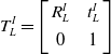 \begin{equation} T_{L}^{I}=\left[\begin{array}{c@{\quad}c} R_{L}^{I} & \mathit{t}_{L}^{I}\\[4pt] 0 & 1 \end{array}\right] \end{equation}
The following equation holds for any k:
 \begin{equation} T_{I_{k+1}}^{I_{k}}T_{L}^{I}=T_{L}^{I}T_{L_{k+1}}^{L_{k}} \end{equation}
Rewritten Eq. (2) combined with Eq. (1):
 \begin{equation} \mathit{R}_{I_{k+1}}^{I_{k}}R_{L}^{I}=R_{L}^{I}\mathit{R}_{L_{k+1}}^{L_{k}} \end{equation}
 \begin{equation} \left(\mathit{R}_{I_{k+1}}^{I_{k}}-I \right)\mathit{t}_{L}^{I} = R_{L}^{I}\mathit{t}_{L_{k+1}}^{L_{k}}-\mathit{t}_{I_{k+1}}^{I_{k}} \end{equation}
Using quaternion instead of rotation matrices, Eq. (3) can be written as:
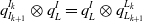 \begin{equation} \mathit{q}_{I_{k+1}}^{I_{k}}\otimes q_{L}^{I}=q_{L}^{I}\otimes \mathit{q}_{L_{k+1}}^{L_{k}} \end{equation}
Rewritten as left-multiply and right-multiply form:
 \begin{equation} \left[Q_{1}\left(\mathit{q}_{I_{k+1}}^{I_{k}}\right)-Q_{2}\left(\mathit{q}_{L_{k+1}}^{L_{k}}\right)\right]\cdot q_{L}^{I}=Q_{k+1}^{k}\cdot q_{L}^{I}=0 \end{equation}
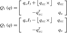 \begin{equation} \begin{array}{c} Q_{1}\left(\mathit{q}\right)=\left[\left.\begin{array}{c@{\quad}c} q_{\omega }I_{3}+\left\lfloor q_{xyz}\times \right\rfloor & q_{xyz}\\[8pt] -q_{xyz}^{T} & q_{w} \end{array}\right]\right.\\[13pt] Q_{2}\left(\mathit{q}\right)=\left[\left.\begin{array}{c@{\quad}c} q_{\omega }I_{3}-\left\lfloor q_{xyz}\times \right\rfloor & q_{xyz}\\[8pt] -q_{xyz}^{T} & q_{w} \end{array}\right]\right. \end{array} \end{equation}
In the above formula, $q_{xyz}$
takes the imaginary part of the quaternion
$q_{xyz}$
takes the imaginary part of the quaternion $q$
and
$q$
and $q_{\omega }$
takes its real part. There is a linear equation system corresponding to n groups of measurement values as follows:
$q_{\omega }$
takes its real part. There is a linear equation system corresponding to n groups of measurement values as follows:
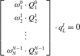 \begin{equation} \left[\left.\begin{array}{c} \omega _{1}^{0}\cdot \mathit{Q}_{1}^{0}\\[4pt] \omega _{2}^{1}\cdot \mathit{Q}_{2}^{1}\\[4pt] \vdots \\[4pt] \omega _{N}^{N-1}\cdot \mathit{Q}_{N}^{N-1} \end{array}\right]\right.\cdot q_{L}^{I}=0 \end{equation}
where $\omega _{i+1}^{i}$
is the weight of each set of transformation equations, determined by the angular interpolation of the transformation vector between the adjacent LiDARs and the transformation vector derived by the IMU. Through singular value decomposition, the rotational external parameter of LiDAR and IMU
$\omega _{i+1}^{i}$
is the weight of each set of transformation equations, determined by the angular interpolation of the transformation vector between the adjacent LiDARs and the transformation vector derived by the IMU. Through singular value decomposition, the rotational external parameter of LiDAR and IMU $q_{L}^{I}$
can be obtained. By substituting the result of the rotational external parameter into Eq. (4), the translation vector between LiDAR and IMU can be obtained.
$q_{L}^{I}$
can be obtained. By substituting the result of the rotational external parameter into Eq. (4), the translation vector between LiDAR and IMU can be obtained.
RTK (real-time kinematics) differential technique can help improve GNSS’s accuracy and reliability. The antennas and combined navigation modules used in this paper need to be calibrated according to the antenna phase center calibration method [Reference Lukasz, Jacek, Bartosz, Martina and Kamil35] before use. After calibration, the positioning accuracy can reach the centimeter level in an open environment. Hardware synchronization is not applied in the paper. The timestamp for each sensor data is set to the time the data is received.
3. System overview
Aiming at the problem of smooth and accurate positioning for outdoor navigation, we propose an outdoor LiDAR-Inertial SLAM using ground constraints as shown in Fig. 1. The data preprocessing module includes ground point extraction and point cloud clustering to remove outliers and abnormal points, point cloud distortion removal, and IMU pre-integration processing. The extracted ground points are fitted into a plane, which is added to the back-end optimization as a height constraint to improve the positioning accuracy. When the system is initialized, the corresponding keyframe strategy is selected according to the state of the system to ensure a smooth and accurate initial pose and to increase the loop detection efficiency.
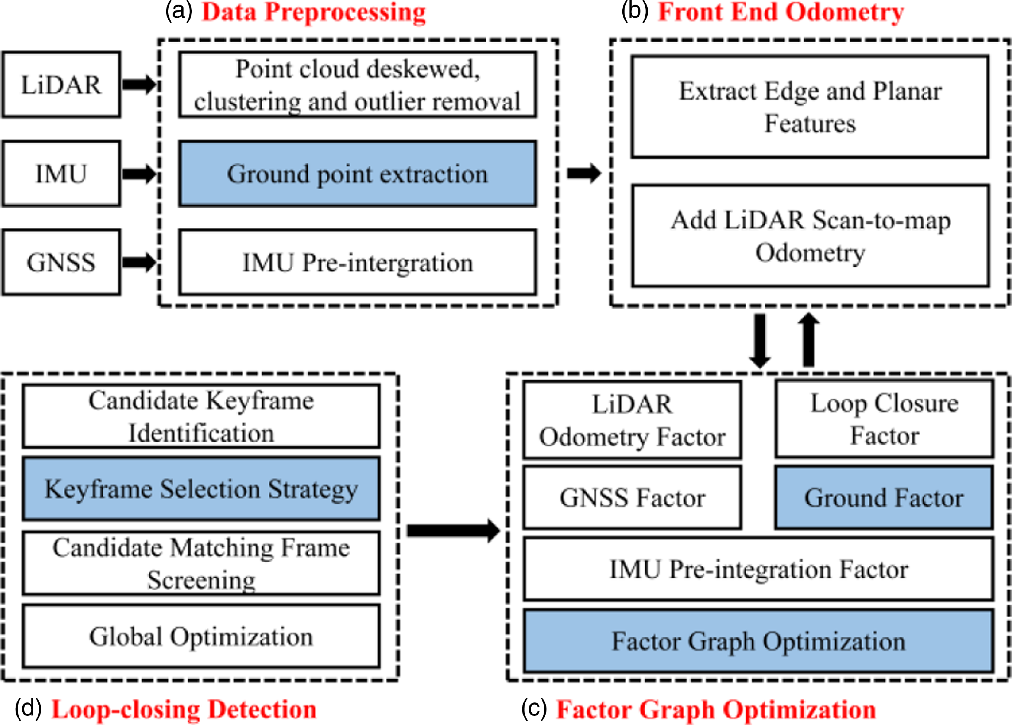
Figure 1. The overall system of the proposed method.
3.1. Data preprocessing
Due to the LiDAR carrier’s or object’s movement, the coordinate system of the start and end moments of the laser beam deviates, and the collected point cloud data are severely distorted. Point cloud de-skewing is performed by fusing the IMU data to obtain the transformation matrix of the end moment relative to the start moment of the laser beam [Reference Zhang and Singh13].
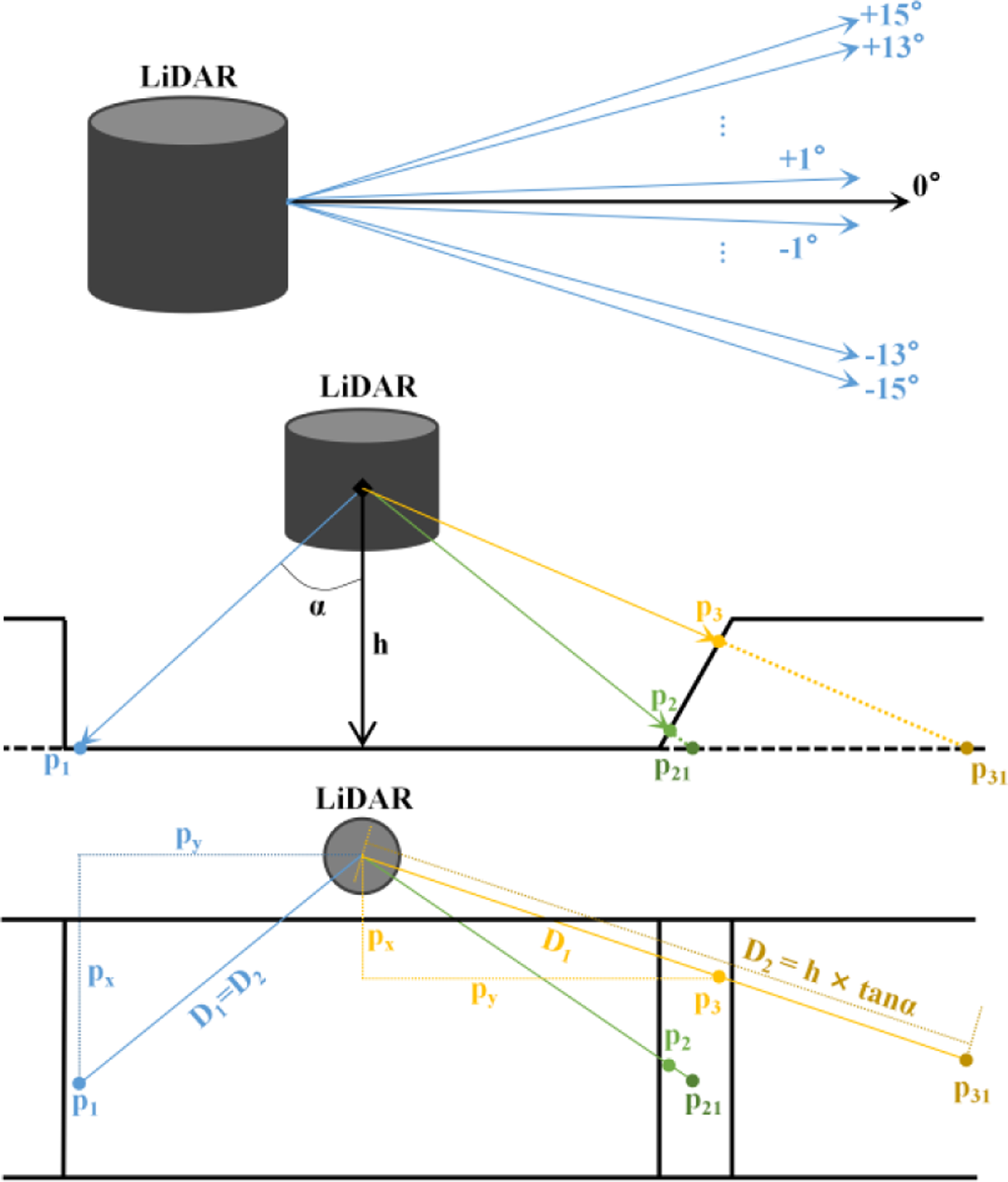
Figure 2.
The upper figure is the definition of the pitch angle of the RS-LiDAR-16, and the middle and lower figures are the ground measurement model of LiDAR when a robot moves on flat ground (the lines of different colors represent different LiDAR beams, and $p_{2}$
and
$p_{2}$
and $p_{3}$
are not ground points as
$p_{3}$
are not ground points as $| D_{2}-D_{1}| \lt \delta$
is not satisfied).
$| D_{2}-D_{1}| \lt \delta$
is not satisfied).
To extract ground points accurately and efficiently, the LiDAR prior installation height and measurement model are used. In a 16-line LiDAR, only the 7 laser beams with a pitch angle of less than 0 are likely to scan the ground. When the robot moves on the plane, the coordinates of the point of the LiDAR beam on the jth (1 ≤ j ≤ 7) line in space $p_{i}$
are set as
$p_{i}$
are set as $(p_{x},p_{y},p_{z})$
. Then, the projection value from the point to the LiDAR on the XY plane
$(p_{x},p_{y},p_{z})$
. Then, the projection value from the point to the LiDAR on the XY plane $D_{1}$
can be expressed as follows:
$D_{1}$
can be expressed as follows:
 \begin{equation} D_{1}=\sqrt{{p_{x}}^{2}+{p_{y}}^{2}} \end{equation}
As shown in Fig. 2, according to the definition of the LiDAR pitch angle, given the angle between the beam and vertical direction, and the installation height $h$
, the projection value from the theoretical point on the ground to the LiDAR on the XY plane
$h$
, the projection value from the theoretical point on the ground to the LiDAR on the XY plane $D_{2}$
can be calculated as:
$D_{2}$
can be calculated as:
 \begin{equation} \alpha =75^{\circ }+\left(j\times 2\right) \end{equation}
 \begin{equation} D_{2}=h\times \tan \alpha \end{equation}
If the point is on the ground, as shown in Fig. 2, D1 and D2 should be equal. The point cloud that satisfies the following formula is marked as the ground point:
 \begin{equation} \left| D_{2}-D_{1}\right| \lt \delta \end{equation}
The threshold $\delta$
is set to determine whether a point is on the ground or not. As shown in the upper figure of Fig. 2, since 7 laser beams have different
$\delta$
is set to determine whether a point is on the ground or not. As shown in the upper figure of Fig. 2, since 7 laser beams have different $\alpha$
, different values of
$\alpha$
, different values of $\delta$
are set for points on different laser beams. If the
$\delta$
are set for points on different laser beams. If the $\alpha$
is larger, the difference between D1 and D2 is allowed to be larger. The constant parameter
$\alpha$
is larger, the difference between D1 and D2 is allowed to be larger. The constant parameter $s$
is obtained according to the actual results of ground point extraction. In this paper, it is set as 0.6.
$s$
is obtained according to the actual results of ground point extraction. In this paper, it is set as 0.6.
 \begin{equation} \delta =\frac{j}{7}\times s \end{equation}
Point cloud clustering removes noise from the environment by classifying adjacent points as identical objects. Horizontal downsampling is performed if the objects are too small to meet the requirement. Based on the labeled point cloud data, edge features and planar features are extracted by calculating the smoothness of the point [Reference Zhang and Singh14]. The smoothness of the point is calculated as follows:
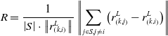 \begin{equation} R=\frac{1}{\left| S\right| \cdot \left\| r_{\left(k,i\right)}^{L}\right\| }\left\| \sum _{j\in S,j\neq i}\left(r_{\left(k,j\right)}^{L}-r_{\left(k,i\right)}^{L}\right)\right\| \end{equation}
S is the set of consecutive points of i returned by the laser scanner at time k.
According to the above calculation, ground features $F_{k}^{g}$
, edge features
$F_{k}^{g}$
, edge features $F_{k}^{e}$
, and planar features
$F_{k}^{e}$
, and planar features $F_{k}^{p}$
are extracted from a LiDAR scan at time k to form a LiDAR frame
$F_{k}^{p}$
are extracted from a LiDAR scan at time k to form a LiDAR frame $\mathrm{\mathbb{F}}_{k}$
.
$\mathrm{\mathbb{F}}_{k}$
.
3.2. Front-end odometry
Some LiDAR keyframes in the past were selected and converted to the robot world coordinate system using the transform associated with them. ${}^{\prime}{F}{_{k-1}^{g}}, {}^{\prime}{F}{_{k-1}^{e}}$
, and
${}^{\prime}{F}{_{k-1}^{g}}, {}^{\prime}{F}{_{k-1}^{e}}$
, and ${}^{\prime}{F}{_{k-1}^{p}}$
are the transformed features in the world coordinate system. The voxel map
${}^{\prime}{F}{_{k-1}^{p}}$
are the transformed features in the world coordinate system. The voxel map $M_{k-1}$
is constructed using some recently transformed keyframes, which consists of three sub-voxel maps of ground, edge, and planar features.
$M_{k-1}$
is constructed using some recently transformed keyframes, which consists of three sub-voxel maps of ground, edge, and planar features.
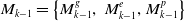 \begin{equation} M_{k-1}=\left\{M_{k-1}^{g},\right.M_{k-1}^{e},\left.M_{k-1}^{p}\right\} \end{equation}
 \begin{equation} M_{k-1}^{\chi }={}^{\prime}{F}{_{k-1}^{\chi }}\cup {}^{\prime}{F}{_{k-2}^{\chi }}\cup \cdots \cup {}^{\prime}{F}{_{k-n}^{\chi }},\chi =g,e,p \end{equation}
A newly acquired LiDAR keyframe $\mathrm{\mathbb{F}}_{k}$
can be firstly converted to the world coordinate system as
$\mathrm{\mathbb{F}}_{k}$
can be firstly converted to the world coordinate system as $\mathrm{\mathbb{F}}^{\prime}_{k}$
using predicted motion
$\mathrm{\mathbb{F}}^{\prime}_{k}$
using predicted motion $\widetilde{T_{I_{k}}^{W}}$
from IMU. The matching method in ref. [Reference Zhang and Singh14] is chosen to find the corresponding features in
$\widetilde{T_{I_{k}}^{W}}$
from IMU. The matching method in ref. [Reference Zhang and Singh14] is chosen to find the corresponding features in $M_{k-1}$
for each feature in
$M_{k-1}$
for each feature in $\mathrm{\mathbb{F}}^{\prime}_{k}$
. The distance of a feature to its corresponding edge
$\mathrm{\mathbb{F}}^{\prime}_{k}$
. The distance of a feature to its corresponding edge $d_{{e_{i}}}$
or plane match
$d_{{e_{i}}}$
or plane match $d_{{p_{j}}}$
is calculated in the form of point-to-line or point-to-surface [Reference Shan, Englot, Meyers, Wang, Ratti and Rus22]. Gauss-Newton method can be used to solve this least squares optimization problem as follows:
$d_{{p_{j}}}$
is calculated in the form of point-to-line or point-to-surface [Reference Shan, Englot, Meyers, Wang, Ratti and Rus22]. Gauss-Newton method can be used to solve this least squares optimization problem as follows:
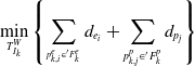 \begin{equation} \min _{T_{I_{k}}^{W}}\left\{\sum _{^{p_{k,i}^{e}\in {}^{\prime}{F}{_{k}^{e}}}}d_{{e_{i}}}+\sum _{p_{k,j}^{p}\in {}^{\prime}{F}{_{k}^{p}}}d_{{p_{j}}}\right\} \end{equation}
The pose transformation of the keyframe at time k in the world coordinate system can be obtained by the above calculation. This transformation is further optimized as a LiDAR odometry factor in factor graph optimization.
3.3. Factor graph optimization
When the robot moves on the horizontal ground, the ground constraint is introduced into the back-end optimization to limit the change in pose between two adjacent keyframes. However, the actual situation is in the scenes of uneven pavement, stone arch bridges, steps, slopes, and other non-horizontal ground. In these cases, the ground constraint is no longer established. When moving on these complex roads, increasing ground constraints may add error information to the back-end optimization process. In this paper, the following two factors are mainly used to determine whether to add ground constraints:
-
1. If the angle between the normal vector of the fitting ground plane $\overset{\rightarrow }{n}$
and the z-axis of the robot
$\beta$
exceeds the given threshold range, it is considered that the mobile robot is not moving on the horizontal ground. From the results of the fitted planes when moving on planar and non-planar surfaces, it is clear that setting the threshold to 10° can be consistent with the actual motion.
$\overset{\rightarrow }{n}$
and the z-axis of the robot
$\beta$
exceeds the given threshold range, it is considered that the mobile robot is not moving on the horizontal ground. From the results of the fitted planes when moving on planar and non-planar surfaces, it is clear that setting the threshold to 10° can be consistent with the actual motion. -
2. Since the experimental scene is an arch bridge of a short length in the campus, the proportion of internal points in the point cloud contained in the current frame
$\rho$
is calculated based on the fitted ground plane. If it is less than a certain threshold of 0.8, the ground is considered uneven. The threshold
$\rho$
is determined based on the results of calculations during multiple motions.


If one of the above conditions is met, the ground constraint is not added to the pose optimization of the back end. On the contrary, if the robot runs on horizontal ground, the corresponding constraints are added to improve the accuracy of the optimization process.
If the ground constraints hold, the ground correspondence of any feature in ${}^{\prime}{F}{_{k}^{g}}$
can be found in
${}^{\prime}{F}{_{k}^{g}}$
can be found in $M_{k-1}^{g}$
. The general equation for the ground plane is solved by constructing the transcendental equation using ground patch correspondence.
$M_{k-1}^{g}$
. The general equation for the ground plane is solved by constructing the transcendental equation using ground patch correspondence.
 \begin{equation} Ax+By+Cz+D=0,A^{2}+B^{2}+C^{2}=1 \end{equation}
The distance from the jth ground point $p_{k,j}^{g}$
at time k to the plane can be constructed as a residual.
$p_{k,j}^{g}$
at time k to the plane can be constructed as a residual.
 \begin{equation} d_{{g_{j}}}=Ax_{k,j}^{g}+By_{k,j}^{g}+Cz_{k,j}^{g}+D \end{equation} $\left(x_{k,j}^{g},y_{k,j}^{g},z_{k,j}^{g}\right)$
are the coordinates of point
$\left(x_{k,j}^{g},y_{k,j}^{g},z_{k,j}^{g}\right)$
are the coordinates of point $p_{k,j}^{g}$
.
$p_{k,j}^{g}$
. $T_{L_{k}}^{W}$
is the pose of the LiDAR at time k in the world coordinate system. Therefore, the Jacobian matrix of the above residuals to LiDAR pose can be decomposed into (1) the Jacobian of residuals
$T_{L_{k}}^{W}$
is the pose of the LiDAR at time k in the world coordinate system. Therefore, the Jacobian matrix of the above residuals to LiDAR pose can be decomposed into (1) the Jacobian of residuals $d_{{g_{j}}}$
to points
$d_{{g_{j}}}$
to points $p_{k,j}^{g}$
, and (2) the Jacobian of points
$p_{k,j}^{g}$
, and (2) the Jacobian of points $p_{k,j}^{g}$
to LiDAR pose
$p_{k,j}^{g}$
to LiDAR pose $T_{L_{k}}^{W}$
.
$T_{L_{k}}^{W}$
.
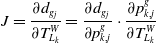 \begin{equation} J=\frac{\partial d_{{g_{j}}}}{\partial T_{L_{k}}^{W}}=\frac{\partial d_{{g_{j}}}}{\partial p_{k,j}^{g}}\cdot \frac{\partial p_{k,j}^{g}}{\partial T_{L_{k}}^{W}} \end{equation}
Jacobi in the first part can be derived from Eq. (19) as the coefficients of the plane equation. The Jacobi of the second part needs to be derived according to the transformation formula of the point from the LiDAR coordinate system to the world coordinate system.
To avoid recalculating the IMU integral after optimizing the bias, IMU pre-integration is applied to obtain the IMU increment between the previous and current frames. $(x_{utm0},y_{utm0},z_{utm0})$
is the UTM coordinate of the first GNSS data.
$(x_{utm0},y_{utm0},z_{utm0})$
is the UTM coordinate of the first GNSS data. $\Phi,\theta$
and
$\Phi,\theta$
and $\psi$
are the roll, pitch, and yaw of the robot’s initial UTM frame. The transform T converts the robot world coordinate system (i.e., the system whose origin is at the starting position of the robot) to the GNSS UTM coordinate system [Reference Thomas and Daniel36]. By taking the LiDAR odometry and GNSS data separately, T can be calculated as follows.
$\psi$
are the roll, pitch, and yaw of the robot’s initial UTM frame. The transform T converts the robot world coordinate system (i.e., the system whose origin is at the starting position of the robot) to the GNSS UTM coordinate system [Reference Thomas and Daniel36]. By taking the LiDAR odometry and GNSS data separately, T can be calculated as follows. $c$
and
$c$
and $s$
stand for cosine and sine functions respectively.
$s$
stand for cosine and sine functions respectively.
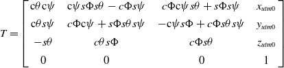 \begin{equation} T=\left[\begin{array}{c@{\quad}c@{\quad}c@{\quad}c} \mathrm{c}\theta \mathrm{c}\psi & \mathrm{c}\mathit{\psi }s\Phi s\theta -c\Phi s\psi & \mathit{c}\Phi \mathrm{c}\psi s\theta +s\Phi s\psi & x_{utm0}\\[4pt] \mathrm{c}\theta s\psi & c\Phi \mathrm{c}\psi +\mathit{s}\Phi s\theta s\psi & -\mathrm{c}\psi s\Phi +\mathit{c}\Phi s\theta s\psi & y_{utm0}\\[4pt] -s\theta & c\theta s\Phi & c\Phi s\theta & z_{utm0}\\[4pt] 0 & 0 & 0 & 1 \end{array}\right] \end{equation}
For any time, the GNSS measurements are transformed to the robot’s world coordinate frame by the following equation. A GNSS factor is added to the system only if the running distance exceeds a certain threshold or if the covariance matrix of the odometry is larger than the covariance of the GNSS.
 \begin{equation} \left[\begin{array}{c} x_{k}^{W}\\[4pt] y_{k}^{W}\\[4pt] z_{k}^{W}\\[4pt] 1 \end{array}\right]=T^{-1}\left[\begin{array}{c} x_{utmk}\\[4pt] y_{utmk}\\[4pt] z_{utmk}\\[4pt] 1 \end{array}\right] \end{equation}
3.4. Loop-closing detection
When the difference between the robot’s current position $T_{I_{k}}^{W}$
and previous position
$T_{I_{k}}^{W}$
and previous position $T_{I_{k-1}}^{W}$
exceeds the defined threshold, the LiDAR frame
$T_{I_{k-1}}^{W}$
exceeds the defined threshold, the LiDAR frame $\mathrm{\mathbb{F}}_{k}$
is selected as the keyframe. The selection of keyframes in this way can achieve a balance between the estimated state of the robot and memory consumption, which is beneficial to improve the accuracy and robustness of the SLAM system. Although it can meet the positioning requirements of small scenes, this keyframe selection strategy still has some problems.
$\mathrm{\mathbb{F}}_{k}$
is selected as the keyframe. The selection of keyframes in this way can achieve a balance between the estimated state of the robot and memory consumption, which is beneficial to improve the accuracy and robustness of the SLAM system. Although it can meet the positioning requirements of small scenes, this keyframe selection strategy still has some problems.
Loop-closing detection is commonly used to mitigate the drift during long-term operation. Based on the point cloud of the current frame, a set of keyframes within the distance threshold will be searched in the KD tree. These candidate keyframes are filtered through feature matching and geometric validation. If the loop-closing is confirmed to be effective, graph optimization is performed to adjust the map and trajectory. After a long period of accumulation of odometry errors, the loop-closing detection fails when it finally returns to the origin.
In a scene with feature degradation, the drift of the pose is to be increased rapidly. To reduce the localization error of the initial state and the accumulated drift for a long time, as shown in Table I, this paper proposes a keyframe strategy, which sets the corresponding keyframe filter conditions according to different system states. During positioning initialization, the threshold for keyframe selection will be lowered, increasing the number of keyframes. In loop-closing detection, the strategy avoids the situation that too few constraints lead to poor matching effect or even non-convergence in feature matching. Thus, it can effectively identify the environment scanned at the beginning and reduce the localization error in large scenes.
Table I. Keyframe selection strategy.

4. Experiments and results
As shown in Fig. 3, the experiments are conducted using the outdoor four-wheeled ground robot. The experimental platform is developed to integrate sensing and computing, including a LiDAR and a nine-axis IMU sensor (RS-LiDAR-16, LPMS-IG1-RS232 series), an Intel Corei9-10900 model (memory 32 GB) on-board computer, and a power supply system. The scanning frequency of the LiDAR sensor is set to 10 Hz for obtaining a horizontal angular resolution of 0.2°. The robot is also equipped with high-precision RTK, which is used to collect the outdoor motion trajectory of the robot when the GNSS data is reliable. For the experiments, the external parameters of the LiDAR and IMU are calibrated using the method described in Section 2.
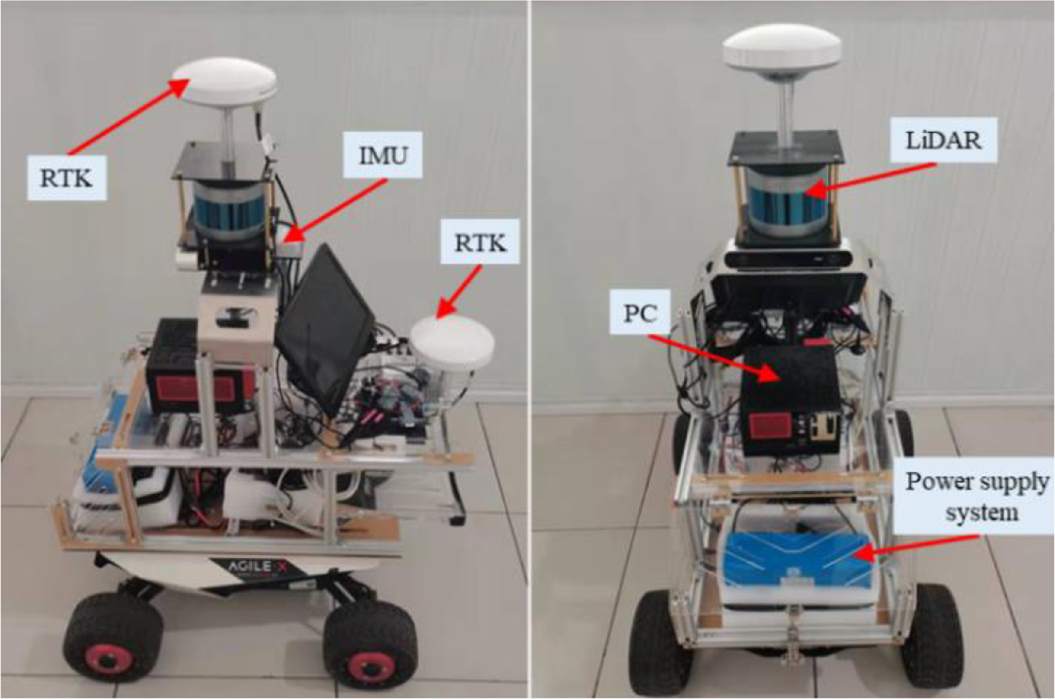
Figure 3. Mobile robot experimental platform.
An outdoor LiDAR-Inertial SLAM is built using ground constraints. The data sets for experiments are collected from a variety of scenes, including scenes with a certain slope, outdoor stone arch bridge, and degradation characteristics. Through the following four experiments (point cloud segmentation, outdoor large scene, positioning initialization, and loop detection), the effect of this method on positioning accuracy in different environments is verified.
4.1. Ground point segmentation
To verify the effectiveness of our proposed ground segmentation algorithm, experiments are carried out in both uphill and downhill scenes. The method proposed by Shan et al. [Reference Shan and Englot15] is relatively simple. It only judges whether the point belongs to the ground according to the height difference of scanning points in the same column of adjacent lines. If it encounters some high planes, it will also be wrongly recognized as the ground. Our method not only considers the installation height of LiDAR but also sets the corresponding threshold according to the number of lines where the scanning points are located. As shown in Fig. 4, the LeGO-LOAM algorithm mistakenly identifies weeds, small trees, and stone arch bridges as ground points, whereas our method performs accurate segmentation. As shown in Fig. 5, our method eliminates a large number of non-ground points, such as mounds, walls, and lower parts of trees. The experimental results prove the accuracy and robustness of this method.
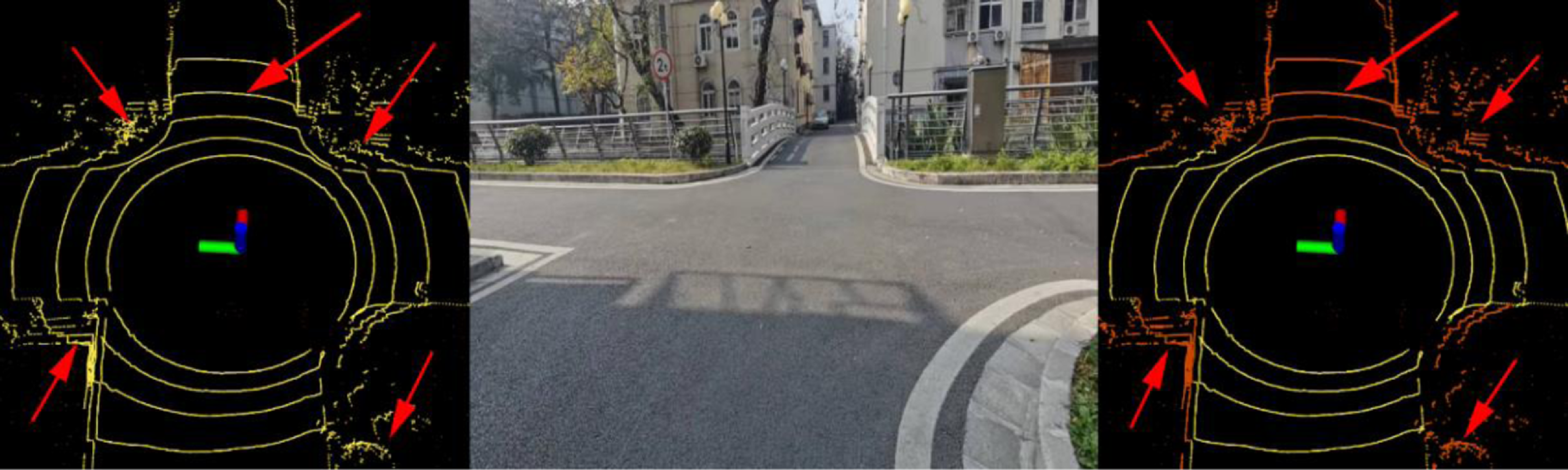
Figure 4. A scene of uphill (the left picture is obtained by the LeGO-LOAM segmentation algorithm, and the right picture is obtained by the method proposed in this paper. The yellow dots are considered ground points).
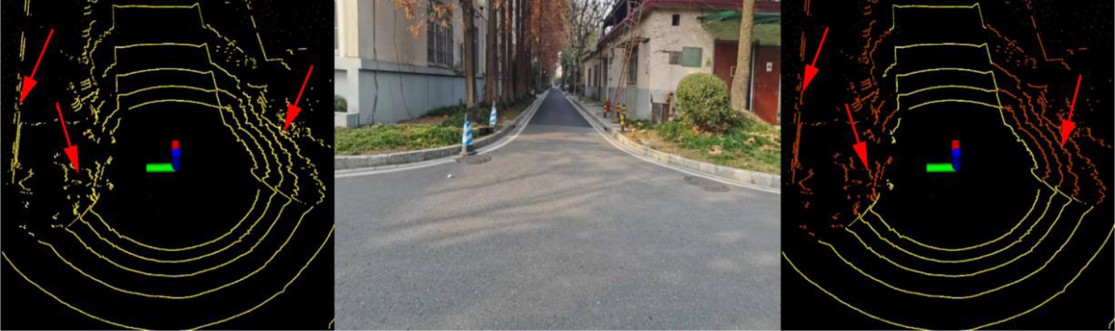
Figure 5. A scene of downhill (The LeGO-LOAM segmentation algorithm is on the left side, and our method is on the right side).
4.2. Outdoor large scene experiment
In order to verify the improvement of the positioning accuracy in the height direction by the ground constraint in the GNSS-limited scene, the experiment is carried out in the scene containing two-stone arch bridges. Accurate trajectory values could not be obtained in this experiment due to the absence of GNSS signals. As shown in Fig. 6(a), the mobile robot returns to the origin counterclockwise with a total path length of 327 m. The loop detection function is turned off during the operation. As the robot eventually returns to its initial position in the experiment, the final robot position is anticipated to be close to the origin of the trajectory. The motion trajectories obtained by different algorithms are shown in Fig. 6(b). Further, as shown in Fig. 7, there are displacement curves in different directions. The LIO-SAM grows the displacement in height rapidly, reaching 8 m after arriving at Bridge A. The displacement decreases rapidly after passing Bridge B. This result is very different from the case that the robot predominantly moves on a horizontal road surface, except for the bridges. Upon the robot eventually returning to its initial point, the height error of LIO-SAM is measured at 2.14 m, markedly surpassing the error of our algorithm which is 0.92 m. Our method adds corresponding ground constraints to the factor graph optimization according to the actual motion, reducing the error in the height direction. Experimental results show that the accuracy of robot positioning is effectively improved when moving in outdoor environments.
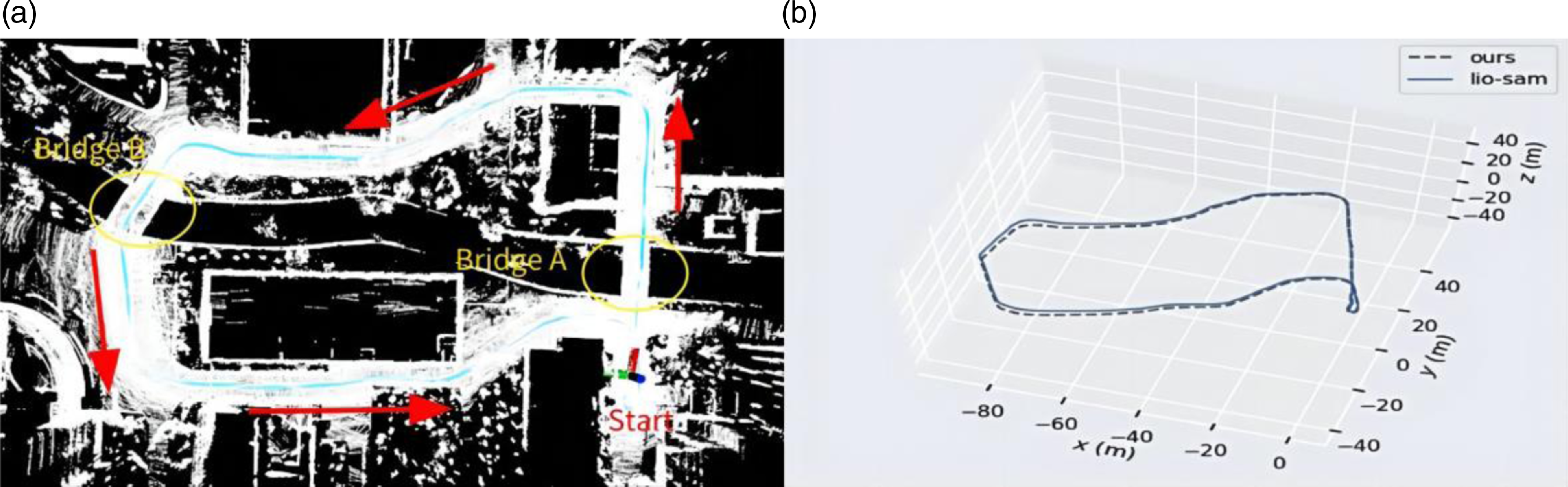
Figure 6. (a) 3D point cloud and (b) trajectory comparison of different algorithms.
Table II. Absolute trajectory errors(m) of each axis of different algorithms in a real scenario.
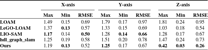
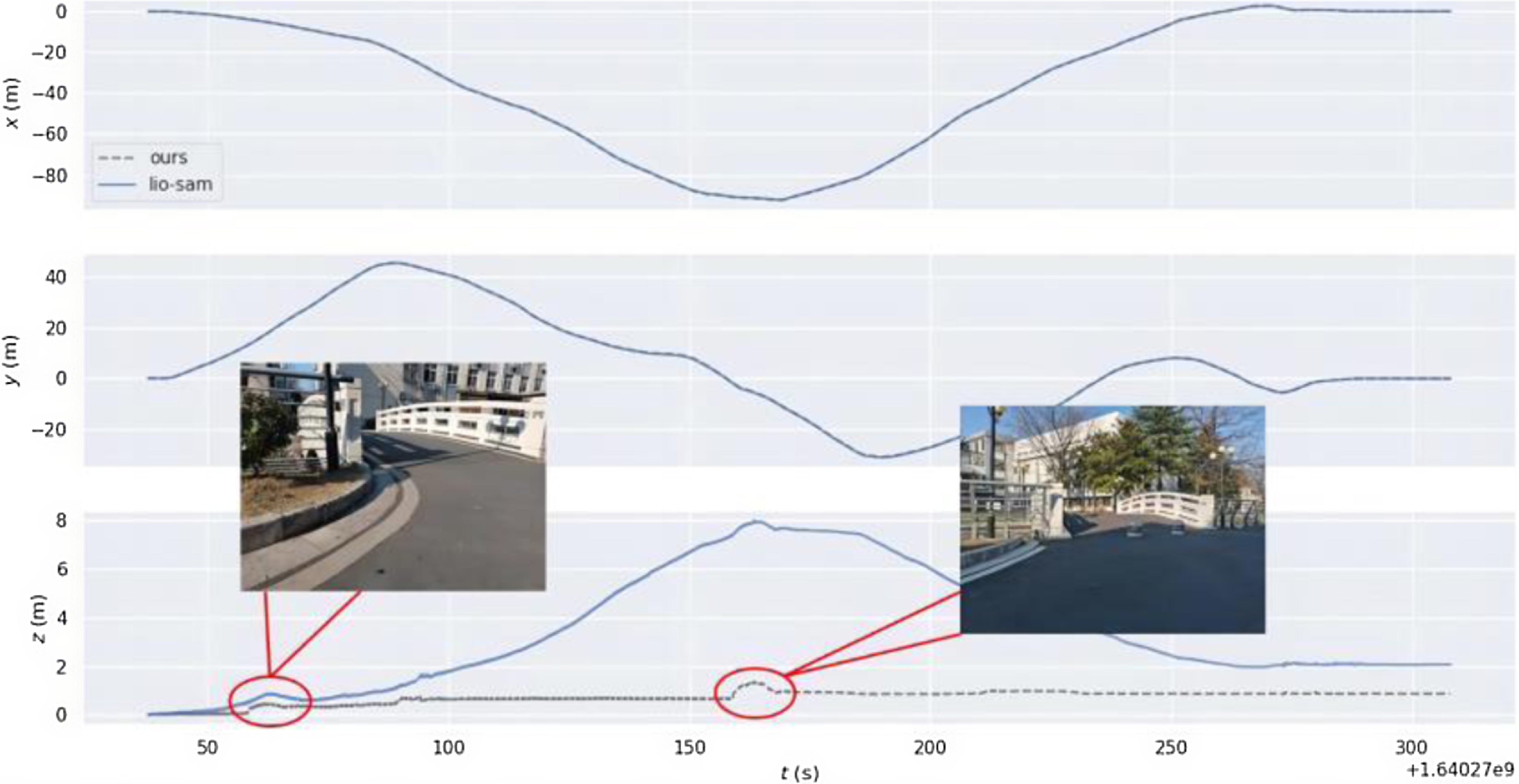
Figure 7. Variation curve of displacement along each axis.
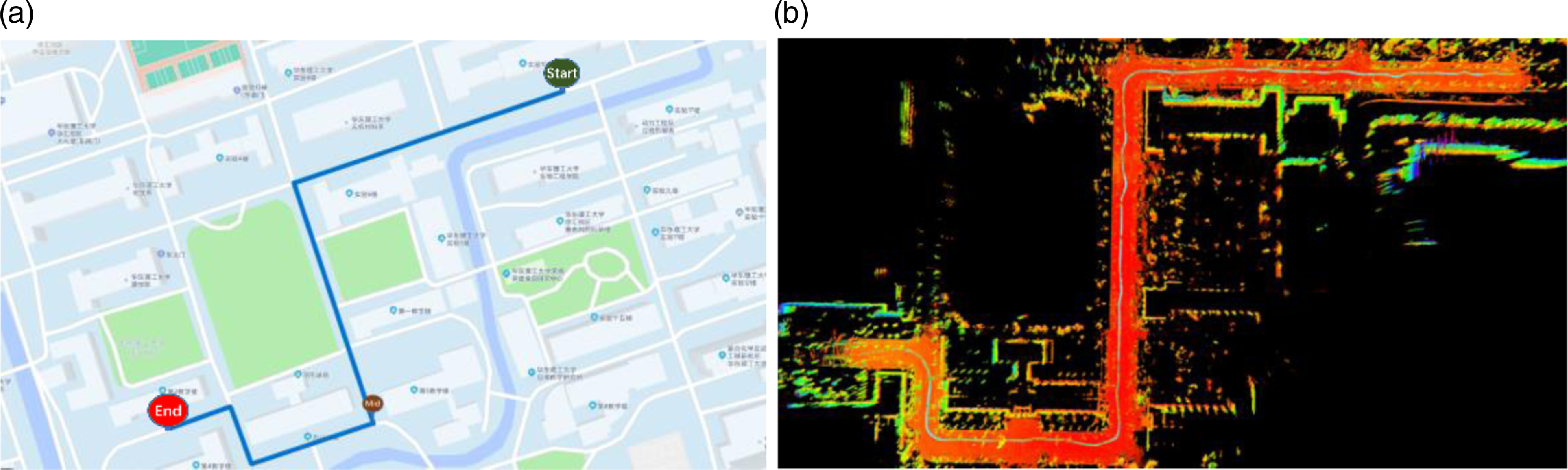
Figure 8. (a) The planning path of the experiment and (b) 3D point cloud of our algorithm.
To prove the effect of ground constraint in large scene motion, the experiment was carried out according to the path shown in Fig. 8 (a). LiDAR and IMU data are collected simultaneously, and the GNSS data are obtained as the truth value of the trajectory. The open sources of LOAM, LeGO-LOAM, LIO-SAM, and hdl-graph-slam [Reference Kenji, Jun and Emanuele37] are used to obtain the trajectories and to measure the errors in the experiments. Hdl-graph-slam is a graph optimization-based SLAM approach that introduces GPS position constraints for outdoor environments. For a fair comparison, all algorithms use only LiDAR and IMU data. The error data of each axis of different algorithms are counted, as shown in Table II. IMU data in LOAM and LeGO-LOAM are only used for distortion removal of point clouds. Since no loopback occurs, the error of the proposed algorithm in the x and y axes is close to that of other algorithms. Due to the addition of ground constraints, the positioning accuracy of our proposed algorithm in the Z-axis is higher than other algorithms.
4.3. Positioning initialization
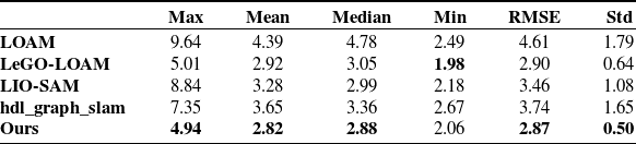
In this experiment, the improved effect of the keyframe selection strategy on the initial positioning error is verified. As shown in the first row in Fig. 9, the mobile robot makes a clockwise circle and then returns to the origin in the campus environment. The track length is 590 m and the duration is 251s. As depicted in the sub-figure of the lower left in Fig. 9, the green line corresponds to the output generated by the LIO-SAM, while the blue line represents the actual trajectory obtained by RTK. The experimental results show that during the initialization process, the LIO-SAM algorithm faces a large cumulative error from the beginning of the movement to the time when the number of keyframes is not zero. After receiving the GNSS data, the pose is optimized and adjusted. At this moment, the positioning changes greatly, which is difficult to meet the continuity requirements of positioning in outdoor autonomous navigation. In this paper, more keyframes are reasonably added at the initial stage of the system, so that a continuous and accurate pose can be obtained. After completing the initialization state, the threshold values of displacement and rotation are automatically adjusted to reduce the resource consumption caused due to the selection of too many keyframes. In addition, as shown in the second row in Fig. 9, since our method extracts more keyframes near the starting point, the set of keyframes close to the current frame is increased during the loopback, which further improves the positioning accuracy and consistency of trajectory. The absolute trajectory errors of localization for different algorithms in this scenario are shown in Table III.
Table III. Absolute trajectory errors(m) of different algorithms in a real scenario.
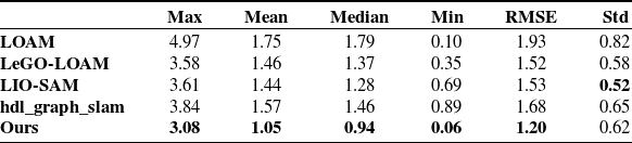
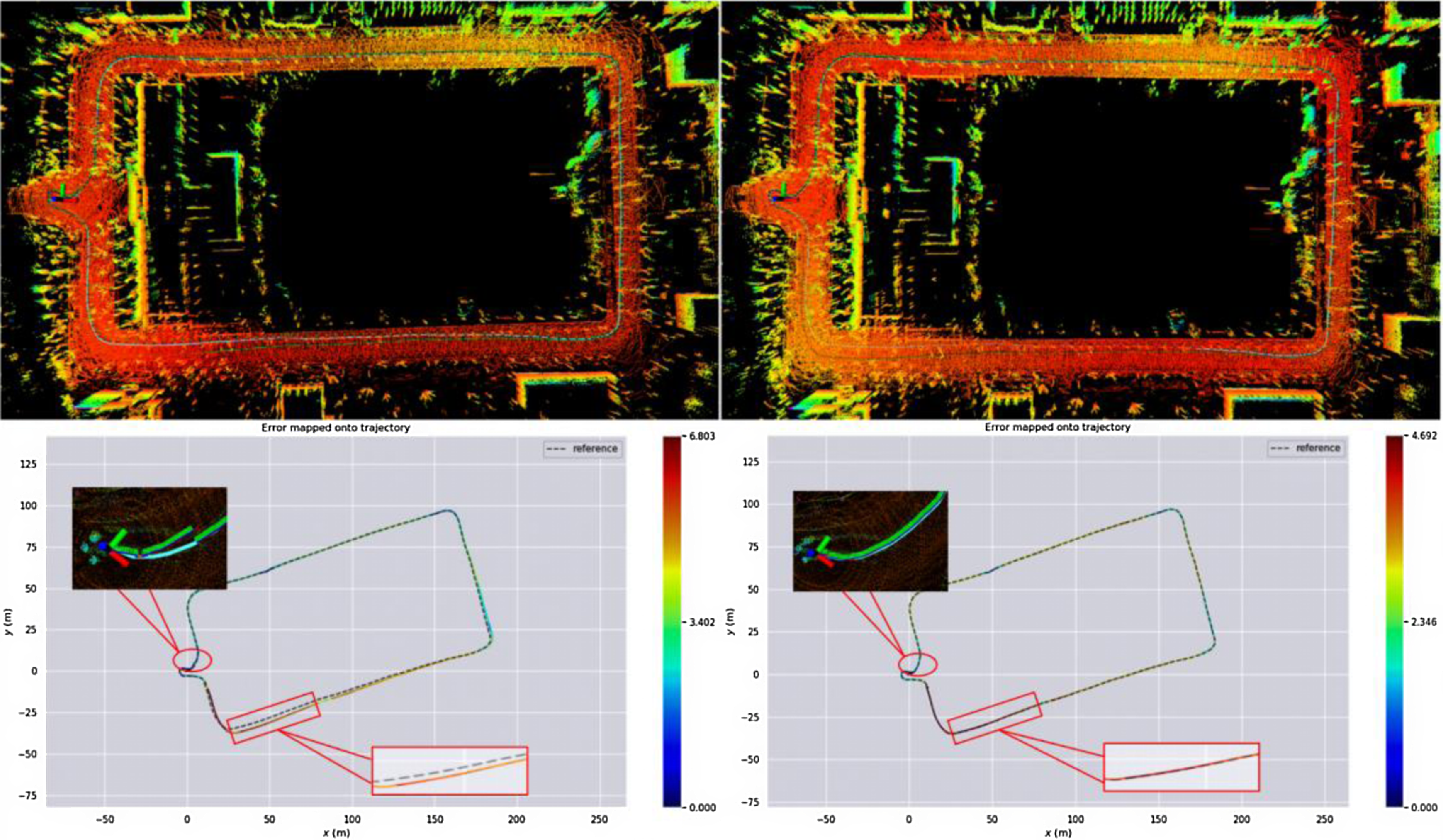
Figure 9. Point cloud image of LIO-SAM (upper left), point cloud image of the method proposed in this paper (upper right), and the corresponding absolute trajectory error with GNSS (lower part).
In addition, our proposed algorithm and other algorithms are tested on the KITTI data set. The experiments are performed on the dataset numbered 2011_09_30_drive_0018, and the absolute trajectory errors are evaluated. Table IV shows that most data related to our algorithm’s absolute trajectory error are smaller than others, which indicates the localization performance of our algorithm is better than others in this data set. This is mainly because our proposed algorithm inhibits error growth in the Z-axis direction.
Table IV. Absolute trajectory errors(m) of different algorithms on the KITTI data set.
4.4. Loop detection
In order to verify the improvement in positioning accuracy of this method when the GNSS signal is limited, only the LiDAR point cloud and IMU data are used. As shown in Fig. 10, the mobile robot moves clockwise back to the origin, with a total length of 953 m. The elliptical marking area is a narrow and long road section formed by the building. As shown in Fig. 11, when passing through two characteristic degradation environments, the displacement change in the z-axis direction increases rapidly. In the point cloud generated by the LIO-SAM due to the continuous accumulation of errors in the process of movement, no loop is detected after returning to the starting point. Our method reasonably introduces ground constraints according to the state of the ground during the movement of the mobile robot, which effectively reduces the continuous accumulation of height errors. At the same time, more keyframes are reserved during the positioning initialization. After moving to the origin, the candidate loopback frames can be effectively detected, and more adjacent keyframes can be obtained to form a local map. In the process of using the iterative closest point, it can effectively converge from the current frame to the local map, and get good enough matching results. Compared with the original LIO-SAM method, this proposed method significantly improves the positioning accuracy in the height direction.
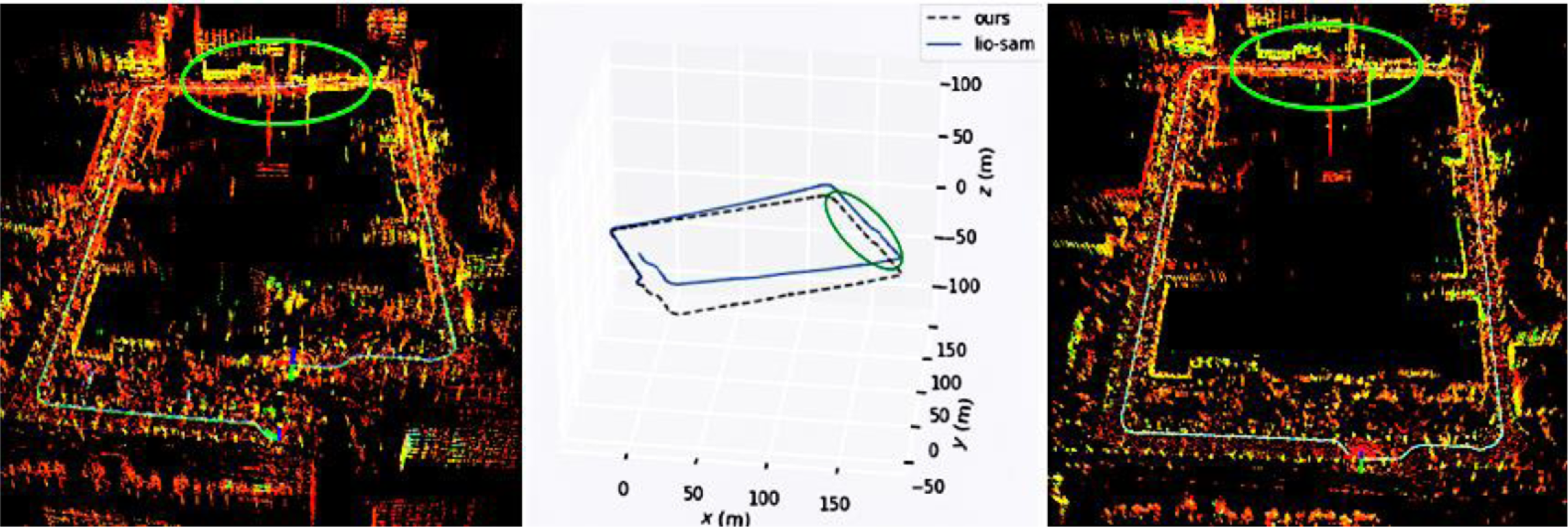
Figure 10. Point cloud generated by the LIO-SAM algorithm (left), trajectory comparison of the two algorithms (middle), and point cloud generated by the algorithm proposed in this paper (right).
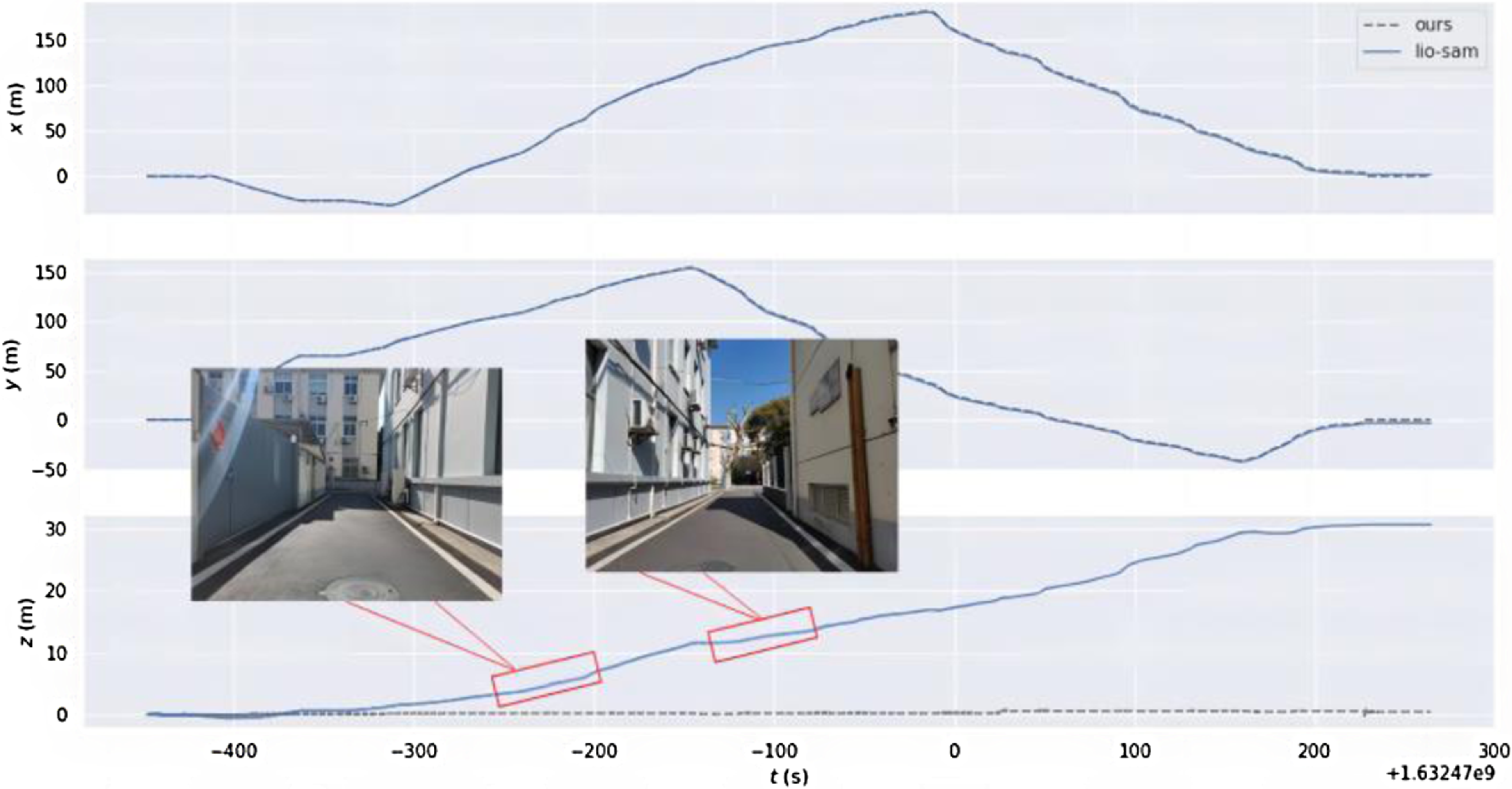
Figure 11. Variation curve of displacement along each axis.
5. Conclusion
To reduce the large Z-axis error caused by grand movement, an outdoor fusion positioning method is proposed. The framework adds LiDAR and IMU to a tightly coupled factor graph and introduces global observations when GNSS data are available. A new method of ground segmentation is proposed, which can obtain good segmentation performance even in cluttered scenes. When the ground condition is satisfied, the ground constraint is added to the factor graph optimization. In addition, to effectively reduce the positioning error in the initial state, a keyframe selection strategy is proposed. It adjusts and optimizes the threshold of keyframe selection according to different states of the system and retains more keyframes at the starting point. A large number of experiments have been carried out on the self-developed robot platform. In Section 4, ground segmentation experiments are first conducted in uphill and downhill scenarios to verify the proposed segmentation algorithm. Secondly, the results of our algorithm are compared with those of other algorithms in GNSS-constrained environments to demonstrate that the proposed ground constraints are effective in reducing the Z-axis error. Then, experiments on campus environments and data sets are performed. The absolute trajectory errors of different algorithms are evaluated to prove the effectiveness of the keyframe strategy and ground constraints. In addition, loop closure is turned on in the experiment in Section 4.4, which verifies that the algorithm can correctly detect the loop to eliminate the cumulative error of long-term operation.
Experiments show that the proposed algorithm is suitable for outdoor large-span environments and can effectively reduce cumulative error. However, some problems faced in this paper still need to be solved. In scenes with fewer edge features, cameras can be added to the proposed framework to extract richer information from the environment and better deal with complex environments. By making full use of environmental information and installing sensors, it is expected to achieve more powerful slam systems.
Acknowledgements
The authors would like to express their gratitude to EditSprings (https://www.editsprings.cn) for the expert linguistic services provided.
Author contributions
Liu Shuang conceived the study, Hu Yating and Zhou Qigao conducted specific experiments and analyses with Miao Zhejun and Yuan Hang’s help, and the two wrote the paper together.
Financial support
This work is supported by Innovation Program of Shanghai Municipal Education Commission (2019-01-07-00-02-E00068).
Competing interests
The authors declare no competing interests exist.
Ethical approval
Not applicable.


