


1. Introduction
In the past years, collaborative robots have transformed the manufacturing sector in a positive way due to its advantages of safety, accuracy, flexibility and lead-through programming [Reference Madsen, Rosenlund, Brandt and Zhang1, Reference Zhuang, Guan, Xu and Dai2], and they also have brought about affordable solutions to mass customization and small-scale manufacturing such as complex assembly, carving and surgery [Reference Althoff, Giusti, Liu and Pereira3–Reference Hong and Rozenblit5]. Collaborative robots are becoming intelligent assistants for human in industrial settings and daily lives.
In all these applications, collaborative robots frequently interact with human or environment, and thus, accurate dynamic modeling is prerequisite for robot control. There are two main reasons for this. One is that precise dynamic modeling can be used in detecting contact forces so that the controlling precision and the safety of physical human-robot interactions can be effectively guaranteed [Reference Hu and Xiong6]. The other is that the dynamic modeling-based force compensation can allow non-experts to achieve correct lead-through programming for rapidly deployed collaborative robots [Reference Althoff, Giusti, Liu and Pereira3].
However, the dynamic system is affected by a variety of parameters such as the link inertia tensor, mass, mass center, joint friction, etc. Although these parameters can generally be tested through CAD (computer-aided-design) software, their real values are in fact unequal to theoretical values due to many factors including production, assembly and aging of robots. Thus, an identification approach was proposed to characterize the dynamic model more accurately [Reference Golluccio, Gillini, Marino and Antonelli7].
When model identification is represented as a linear regression problem, the ordinary least-squares (LS) is frequently used as an identification approach. It yields a numerical solution by minimizing the square of errors. And then its derivatives are used to build the weighted least-squares (WLS) for purpose of reducing the sensitivity of the algorithm to system noise [Reference Gautier8, Reference Gautier and Poignet9]. However, the results of the LS-based approach are highly biased and may be physically infeasible [Reference Leboutet, Roux, Janot, Guadarrama-Olvera and Cheng10]. For example, it can yield negative mass parameters occasionally. These physically infeasible estimates will lead to unrealistic simulations or inherently unstable model-based control [Reference Hu and Xiong6, Reference Han, Wu, Liu and Xiong11].
In recent years, the convex optimization techniques with inequality constraints have been adopted to guarantee the physical consistency of parameters. Sousa [Reference Sousa and Cortesão12] defined the feasibility conditions as a convex set in the form of a linear matrix inequality (LMI) that can be applied in semidefinite programming (SDP) algorithm. Based on LMI-SDP, Jung [Reference Jung, Cheong, Park and Park13] put forth a backward sequential method to optimize the identification speed when models have large degrees of freedom (DOF). The LMI-SDP algorithm can also be combined with non-parametric compensators to construct a semi-parametric dynamic model to improve the model’s accuracy [Reference Hu and Xiong6]. Owing to the manifold constraints that can be projected as convex constraints through LMI, Wensing [Reference Wensing, Kim and Slotine14] reformulated physical-consistency constraints of inertial parameters as LMI and verified a necessary and sufficient condition for its density realizability on an ellipsoid. Lee [Reference Lee, Wensing and Park15] proposed a geometric programming approach based on the Riemannian structure of positive definite matrices, which enables semidefinite optimization for convex regularization of parameter estimates. Then, Janot [Reference Janot and Wensing16] developed a sequential semidefinite optimization procedure for ensuring the physical and statistical consistency of the identified model.
Since most collaborative robots rely on geared drives where actuation performance is significantly influenced by frictional effects, it is important to model and identify robots’ joint friction [Reference Iskandar and Wolf17, Reference Tadese, Yumbla, Yi, Lee, Park and Moon18]. Typical friction models describe the joint friction torque as a nonlinear and discontinuous function that generally contains components of Coulomb friction, viscous friction, and Stribeck friction [Reference Althoff, Giusti, Liu and Pereira3, Reference Gautier8, Reference Canudas de Wit, Olsson, Astrom and Lischinsky19, Reference Zhang, Wang, Jing and Tan20]. The real values of friction model parameters may be different from their theoretical value due to wear, aging and deformation of the joints. In practice, these influences can be determined from experimental data. Walter [Reference Walter21] formulated friction model as a linear function of velocity and introduced friction model parameters into a set of dynamic model parameters to be estimated together with others. For purpose of eliminating the influence of biased data near-zero-velocity region on the identification results, an iteratively reweighted least-squares (IRLS) approach was proposed by Han [Reference Han, Wu, Liu and Xiong11]. In IRLS, the WLS, reweighted functions and nonlinear friction models are generally integrated to remove bias data in the near-zero-velocity region with high measurement noise, and finally improve the robustness and accuracy of the algorithm through three iterative loops. Xu [Reference Xu, Fan, Chen, Ng, M.H., Fang, Zhu and Zhao22, Reference Xu, Fan, Fang, Zhu and Zhao23] simplified the IRLS method as two loops and applied it in the dynamic identification on the current level and the payload identification of robots. In IRLS, it can only model the velocity-dependent friction torque of robotic joints, which is insufficient to characterize the variation of friction with the heat-dissipation of motor, ambient temperature change and configural change for collaborative robots [Reference Tadese, Yumbla, Yi, Lee, Park and Moon18, Reference Gao, Yuan, Han, Wang and Wang24].
In Gao [Reference Gao, Yuan, Han, Wang and Wang24] and our previous works [Reference Zeyu, Hongxing, Ziyi and Gang25], it was verified that the angular velocity and temperature of joints have a nonlinear influence on viscous friction, while the load torque significantly influences the Coulomb friction linearly. Gao [Reference Gao, Yuan, Han, Wang and Wang24] proposed a comprehensive mathematical friction model based on the physical properties of lubricant shear stress to estimate these influences with the Levenberg-Marquardt nonlinear least-squares method. Hamon [Reference Hamon, Gautier and Garrec26] identified the load-independent and velocity-dependent friction model by moving one single joint at a time. Janot [Reference Janot27] identified the structure of the load-independent friction models with non-parametric state-dependent-parameter estimations and then they identified inertial parameters with LS, respectively. Simoni [Reference Simoni, Beschi, Legnani and Visioli28] extended the polynomial joint friction-temperature model by considering lubricant viscosity and the Stribeck phenomenon. Then, Madsen [Reference Madsen, Rosenlund, Brandt and Zhang1] proposed a modeling and identification method of nonlinear joint dynamics for collaborative robots. This method describes the most dominant dynamic characteristics of nonlinear joint friction by considering the effects of angular velocity, temperature and load torque. In addition, it extends the Generalized Maxwell-Slip model to represent the observed friction phenomena at near-zero velocities. Hao [Reference Hao, Pagani, Beschi and Legnani29] described the relationship between friction and temperature with a double exponential model and adjusted its parameters by genetic algorithms. However, separated identification of the friction model introduces extra outliers in the near-zero-velocity region, that will lead to bias in the dynamic model identification [Reference Han, Wu, Liu and Xiong11]. Hitherto, how to estimate dynamic model parameters when considering comprehensive friction model factors has been an unsolved challenge for collaborative robots.
In response to the above challenges, this research proposes an improved IRLS (I-IRLS) algorithm for collaborative robots when considering the effects of joint velocity, temperature and load torque on robotic dynamics. The identification framework in the present research consists of four iterative loops: A set of dynamic parameters is obtained by LMI-SDP in the first loop; a reweighted matrix is generated by normalizing the residuals to filter the measured data in the second loop; the joint friction model parameters are estimated by an optimization approach under constraints of feasibility in the third loop; and the priority matrix of the friction model is updated in the fourth loop. Compared with the previous IRLS modeling approach, the contributions of this research can be summarized as follows:
-
A mathematical friction model is developed through experiments on robot joints. It comprehensively characterizes the dependence of friction torque on the joint velocity, temperature and load torque.
-
A globally optimal solution with constraints is applied in dynamic identification. The LMI-SDP is employed to estimate the dynamic parameters set and the interior-point method with multiple starting points is used to calculate the friction model parameters. In this way, one can ensure the physical feasibility of parameters and reduce the influence of initial value on the identification results.
-
An improved iterative identification approach is proposed. It improves the friction model and its solution in the third loop. A new fourth loop is introduced to update the model’s prior knowledge so that the convergence and consistency of the model parameters can be guaranteed.
-
Experiments are conducted on the AUBO collaborative robot, and the estimation error of the proposed algorithm is reduced by at least 14% over those of other existing algorithms.
The rest of this article consists of three sections. Section 2 introduces the process of dynamic identification. Section 3 shows the results of experiments on the AUBO I5 collaborative robots. Section 4 concludes the present work.
2. Method
2.1. Inverse dynamics
The dynamics of a n-DOF serial robot can be expressed as:
 \begin{equation} M(q)\ddot{q} + C(q,\dot{q})\dot{q} + G(q) +{F_{fric}} = \tau +{\tau _{ext}} \end{equation}
where $q \in \mathbb{R}^n$
,
$q \in \mathbb{R}^n$
, $\dot{q} \in \mathbb{R}^n$
,
$\dot{q} \in \mathbb{R}^n$
, $\ddot{q} \in \mathbb{R}^n$
stand for the joint position, velocity and acceleration, respectively.
$\ddot{q} \in \mathbb{R}^n$
stand for the joint position, velocity and acceleration, respectively. $M(q) \in \mathbb{R}^{n \times n}$
,
$M(q) \in \mathbb{R}^{n \times n}$
, $C(q,\dot{q}) \in \mathbb{R}^{n \times n}$
and
$C(q,\dot{q}) \in \mathbb{R}^{n \times n}$
and $G(q) \in \mathbb{R}^{n}$
represent the inertia matrix, the Coriolis/centrifugal matrix and the gravity vector, respectively.
$G(q) \in \mathbb{R}^{n}$
represent the inertia matrix, the Coriolis/centrifugal matrix and the gravity vector, respectively. ${F_{fric}} \in \mathbb{R}^{n}$
and
${F_{fric}} \in \mathbb{R}^{n}$
and $\tau \in \mathbb{R}^{n}$
are the friction torque vector and control torque vector of the joint.
$\tau \in \mathbb{R}^{n}$
are the friction torque vector and control torque vector of the joint. ${\tau _{ext}} \in \mathbb{R}^{n}$
is the external torque vector due to the physical contact with the environment.
${\tau _{ext}} \in \mathbb{R}^{n}$
is the external torque vector due to the physical contact with the environment.
In the case of robot dynamic identification with electric current measured by drive actuation, the joint control torque can be calculated by:
 \begin{equation} \tau = KI \end{equation}
where $I\in \mathbb{R}^{n}$
is the measured joint electric current and
$I\in \mathbb{R}^{n}$
is the measured joint electric current and $K \in \mathbb{R}^{n \times n}$
is a diagonal matrix consisting of the torque constant of motor.
$K \in \mathbb{R}^{n \times n}$
is a diagonal matrix consisting of the torque constant of motor.
2.2. Friction modeling
It is assumed that the friction torques are uncoupled among the joints and the frictional model form is not changed due to assembly of joint modules for collaborative robots [Reference Madsen, Rosenlund, Brandt and Zhang1]. And frictional torque $F_{fric}$
is frequently described as a combination of three components, which characterize the effects of joint angular velocity, temperature and load torque, respectively [Reference Madsen, Rosenlund, Brandt and Zhang1]. Specifically, the friction torque of the i-th joint can be calculated by using a composite model
$F_{fric}$
is frequently described as a combination of three components, which characterize the effects of joint angular velocity, temperature and load torque, respectively [Reference Madsen, Rosenlund, Brandt and Zhang1]. Specifically, the friction torque of the i-th joint can be calculated by using a composite model
 \begin{equation}{F_{fric,i}} ={f_v}({\dot{q_i}}) +{f_T}({\dot{q_i}},{T_i}) +{f_\tau }(q,{\dot{q_i}}), |\dot{q_i}| \geq \delta \dot{q_i} \end{equation}
where $T_i$
represents the joint temperature.
$T_i$
represents the joint temperature. ${f_v}({\dot{q_i}})$
,
${f_v}({\dot{q_i}})$
, ${f_T}({\dot{q_i}},{T_i})$
and
${f_T}({\dot{q_i}},{T_i})$
and ${f_\tau }(q,{\dot{q_i}})$
stand for the dependence of friction torque on velocity, temperature and load torque, respectively.
${f_\tau }(q,{\dot{q_i}})$
stand for the dependence of friction torque on velocity, temperature and load torque, respectively. $\delta \dot{q_i}$
is the minimum resolution of velocity data. Three groups of experiments were conducted on collaborative robots with easy-assemblable joints to investigate these terms.
$\delta \dot{q_i}$
is the minimum resolution of velocity data. Three groups of experiments were conducted on collaborative robots with easy-assemblable joints to investigate these terms.
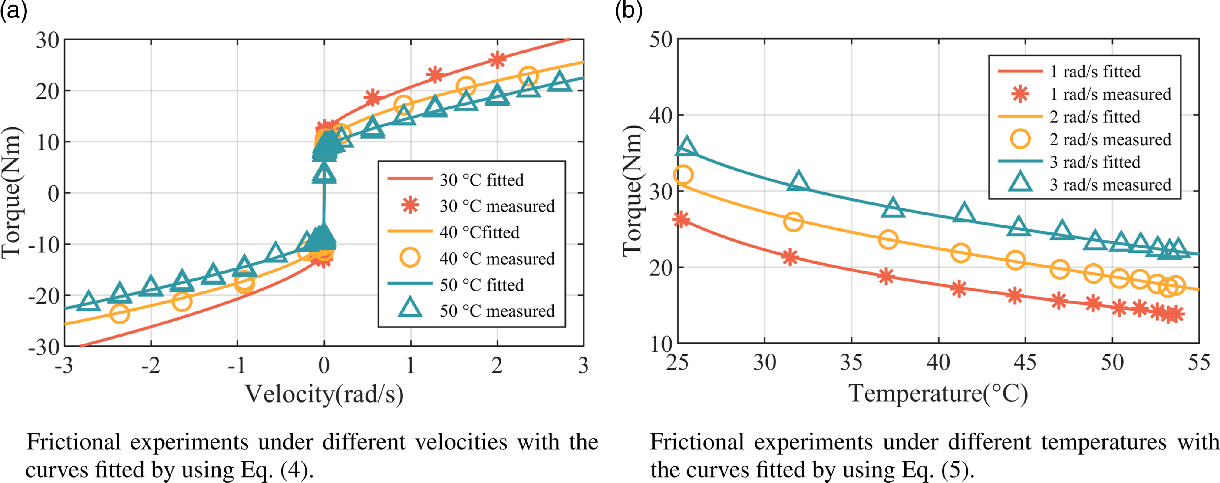
Figure 1. The velocity and temperature dependence of friction.
The first group of experiments were carried out in each single joint with zero load and at a constant temperature to investigate the velocity-dependent friction model. During these experiments, each joint was placed horizontally and driven with a sinusoidally changing speed. The velocity, temperature and driving moment information of the joints were collected during these experiments as shown in Fig. 1(a). Fig. 1(a) indicates that the friction torque increases exponentially with velocity but is discontinuous at near-zero velocities. At different temperatures, the static friction torque almost keeps unchanged, but the viscous friction torque varies significantly as in [Reference Gao, Yuan, Han, Wang and Wang24, Reference Zeyu, Hongxing, Ziyi and Gang25]. Thus, the components, ${f_v}({\dot{q_i}})$
can be described as:
${f_v}({\dot{q_i}})$
can be described as:
 \begin{equation}{f_v}({{\dot{q}}_i}) = [{f_{c,i}} +{f_{v,i}}{\|{{{\dot{q}}_i}}\|^{{\alpha _i}}}]sign({{\dot{q}}_i}) +{f_{{{vo,i}}}} \end{equation}
where $f_{c,i} \gt 0$
represents the Coulomb friction coefficient.
$f_{c,i} \gt 0$
represents the Coulomb friction coefficient. $f_{v,i} \gt 0$
and
$f_{v,i} \gt 0$
and $\alpha _i \gt 0$
are two coefficients that describe the viscous friction behavior.
$\alpha _i \gt 0$
are two coefficients that describe the viscous friction behavior. $f_{{{vo,i}}}$
stands for constant offset.
$f_{{{vo,i}}}$
stands for constant offset.
The second groups of experiments were carried out in each single joint with zero load in an ordinary working environment to investigate the relationship between friction and temperature. A temperature sensor was fixed on the harmonic reducer to measure the joint temperature and each joint was also driven with the same trajectory as the first experiment. In this case, robot joints naturally heat up over 20 $^{\circ }$
C. Fig. 1(b) presents the experimental results, from which it can be seen that temperature-dependent friction is a function of speed and temperature. Therefore, the components
$^{\circ }$
C. Fig. 1(b) presents the experimental results, from which it can be seen that temperature-dependent friction is a function of speed and temperature. Therefore, the components ${f_T}({\dot{q_i}},{T_i})$
of friction torque can be expressed as in [Reference Madsen, Rosenlund, Brandt and Zhang1]:
${f_T}({\dot{q_i}},{T_i})$
of friction torque can be expressed as in [Reference Madsen, Rosenlund, Brandt and Zhang1]:
 \begin{equation}{f_T}({{\dot{q}}_i},{T_i}) = sign({{\dot{q}}_i})\sqrt{\|{{\dot{q}}_i}\|} ({\beta _{1,i}} +{\beta _{2,i}}{T_i} +{\beta _{3,i}}{T_i}^{ - 3}) \end{equation}
where $\beta _{1,i}$
,
$\beta _{1,i}$
, $\beta _{2,i}$
and
$\beta _{2,i}$
and $\beta _{3,i}$
are temperature coefficients.
$\beta _{3,i}$
are temperature coefficients.
The third groups of experiments were introduced to model the relationship between friction and load. During these experiments, each joint was placed horizontally, subjected to a known load and moving at a constant speed in both forward and backward directions, and the joint temperature was kept close to ambient temperature. Fig. 2 indicates the experimental results, from which it can be seen that friction torque has a quadratic-form dependence on the payload torque, and its component ${f_\tau }(q,{\dot{q_i}})$
is expressed as:
${f_\tau }(q,{\dot{q_i}})$
is expressed as:
 \begin{equation}{f_\tau }(q,{\dot{q_i}}) ={f_{L,i}}sign({\dot{q_i}}){\tau _{l,i}}{(q)^2} +{f_{{{lo,i}}}} \end{equation}
where ${\tau _{l,i}}{(q)}$
stands for the load torque of the i-th joint.
${\tau _{l,i}}{(q)}$
stands for the load torque of the i-th joint. $f_{L,i}$
represents a coefficient that describes the effect of joint payload on friction.
$f_{L,i}$
represents a coefficient that describes the effect of joint payload on friction. $f_{{{lo,i}}}$
stands for constant offset and it can be combined with
$f_{{{lo,i}}}$
stands for constant offset and it can be combined with $f_{{{vo,i}}}$
in Eq. (4) to define a unified zero-speed offset as
$f_{{{vo,i}}}$
in Eq. (4) to define a unified zero-speed offset as $f_{{{o,i}}}$
.
$f_{{{o,i}}}$
.

Figure 2. Frictional experiments under different loads with the curves fitted by using Eq. (6).
Remark 1. The variable of ${\tau _{l,i}}{(q)}$
is
${\tau _{l,i}}{(q)}$
is $q$
instead of
$q$
instead of $q_i$
. This is because the load torque of the i-th joint is approximately equal to the i-th component of the dynamic gravity vector, which is related to the robot’s configuration [Reference Ferraguti, Talignani Landi, Sabattini, Bonfè, Fantuzzi and Secchi4, Reference Wahrburg, Bös, Listmann, Dai, Matthias and Ding32].
$q_i$
. This is because the load torque of the i-th joint is approximately equal to the i-th component of the dynamic gravity vector, which is related to the robot’s configuration [Reference Ferraguti, Talignani Landi, Sabattini, Bonfè, Fantuzzi and Secchi4, Reference Wahrburg, Bös, Listmann, Dai, Matthias and Ding32].
2.3. Iterative methodology for dynamic identification
When $\tau _{ext} = 0$
, one compensates the components,
$\tau _{ext} = 0$
, one compensates the components, $f_T$
and
$f_T$
and $f_\tau$
, which are calculated by Eqs. (5) and (6) – with
$f_\tau$
, which are calculated by Eqs. (5) and (6) – with $\alpha _i$
being regarded as a known constant. Then, Eq. (1) becomes
$\alpha _i$
being regarded as a known constant. Then, Eq. (1) becomes
 \begin{equation} M(q)\ddot{q} + C(q,\dot{q})\dot{q} + G(q) +{f_v}(\dot{q}) = \tau ' \end{equation}
and Eq. (1) can be further linearized [Reference Khalil and Kleinfinger30] as:
 \begin{equation} \tau ' = \Phi (q,\dot{q},\ddot{q}){\theta _{linear}} \end{equation}
where $\tau '{\rm{ = }}\tau -{\hat f_T}(\dot{q},T) -{\hat f_\tau }(q,\dot{q})$
.
$\tau '{\rm{ = }}\tau -{\hat f_T}(\dot{q},T) -{\hat f_\tau }(q,\dot{q})$
. $\Phi \in \mathbb{R}^{p \times 13n}$
is a regression matrix,
$\Phi \in \mathbb{R}^{p \times 13n}$
is a regression matrix, $p$
is the sample times and
$p$
is the sample times and ${\theta _{linear}} \in \mathbb{R}^{13n}$
is a parameter vector defined as:
${\theta _{linear}} \in \mathbb{R}^{13n}$
is a parameter vector defined as:
 \begin{equation} \begin{aligned}{\theta _{linear}} &={[{\theta _D}\;{\theta _F}]^T}\\{\theta _D} &={[m\;{S_x}\;{S_y}\;{S_z}\;{I_{xx}}\;{I_{yy}}\;{I_{zz}}\;{I_{xy}}\;{I_{xz}}\;{I_{yz}}]}\\{\theta _F} &={[{f_c}\;{f_v}\;{f_o}]} \end{aligned} \end{equation}
where $\theta _{linear}$
consists of dynamic inertia parameter vector
$\theta _{linear}$
consists of dynamic inertia parameter vector $\theta _D$
and frictional parameter vector
$\theta _D$
and frictional parameter vector $\theta _F$
.
$\theta _F$
. $m$
is the link’s mass.
$m$
is the link’s mass. $S$
and
$S$
and $I$
stand for the first and second-order inertia moments, respectively.
$I$
stand for the first and second-order inertia moments, respectively.
One can perform singular value decomposition or QR decomposition operation on the regression matrix to get the full-rank matrix $\Phi _{min}$
and the minimum parameter set
$\Phi _{min}$
and the minimum parameter set ${\theta _{min}} = \{{\theta _{D,\min }},{\theta _{F,\min }}\}$
.
${\theta _{min}} = \{{\theta _{D,\min }},{\theta _{F,\min }}\}$
. $\theta _{D,\min }$
and
$\theta _{D,\min }$
and $\theta _{F,\min }$
are two re-organized parameter sets of
$\theta _{F,\min }$
are two re-organized parameter sets of $\theta _D$
and
$\theta _D$
and $\theta _F$
, respectively. The symbolic expressions of the minimum parameter set are listed in Appendix.
$\theta _F$
, respectively. The symbolic expressions of the minimum parameter set are listed in Appendix.
By using the minimum parameter set, the dynamic equation can be recast as:
 \begin{equation} \tau ' ={\Phi _{min}}(q,\dot{q},\ddot{q}){\theta _{min}} \end{equation}
For the purpose of reducing the interference of outliers on calculation, the covariance matrix of errors $\Omega$
as defined in [Reference Han, Wu, Liu and Xiong11] is utilized to normalize the regression matrix and respond vector in the first loop (NB: The first loop is the innermost loop denoted as
$\Omega$
as defined in [Reference Han, Wu, Liu and Xiong11] is utilized to normalize the regression matrix and respond vector in the first loop (NB: The first loop is the innermost loop denoted as $L_1$
). Then, the iterative weight vector
$L_1$
). Then, the iterative weight vector $W \in{\mathbb{R}^{mn \times 1}}$
is updated with a T-class hard weight function to gradually remove outliers in the second loop (i.e.,
$W \in{\mathbb{R}^{mn \times 1}}$
is updated with a T-class hard weight function to gradually remove outliers in the second loop (i.e., $L_2$
). Thus, Eq. (10) becomes
$L_2$
). Thus, Eq. (10) becomes
 \begin{equation}{\tau ^{\#} } = \Phi _{min}^{\#} (q,\dot{q},\ddot{q}){\theta _{min}} \end{equation}
and
 \begin{equation} \begin{aligned}{\tau ^{\#} } &= W.*({\Omega ^{ - \frac{1}{2}}} \cdot \tau ')\\ \Phi _{min}^{\#} &={W_e}.*({\Omega ^{ - \frac{1}{2}}} \cdot{\Phi _{min}}) \end{aligned} \end{equation}
where $W_e \in{\mathbb{R}^{mn \times p}}$
is an extension matrix consisting of p-column vectors
$W_e \in{\mathbb{R}^{mn \times p}}$
is an extension matrix consisting of p-column vectors $W$
.
$W$
.
When the solution of Eq. (11) is considered as the result of a linear regression process, the solution of $\hat{\theta }$
can be estimated by using LS to minimize the squared residuals. When the physical feasibility of the solution of Eq. (11) is considered, the constraints of parameters can be written in the form of LMI. Then, a convex optimization problem is reached, and it can be solved by using the SDP technique [Reference Sousa and Cortesão12].
$\hat{\theta }$
can be estimated by using LS to minimize the squared residuals. When the physical feasibility of the solution of Eq. (11) is considered, the constraints of parameters can be written in the form of LMI. Then, a convex optimization problem is reached, and it can be solved by using the SDP technique [Reference Sousa and Cortesão12].
In this case, the normalized error is calculated by
 \begin{equation}{\mathcal{R}^{\#} } ={\tau ^{\#} } - \Phi _{min}^{\#} (q,\dot{q},\ddot{q}){\hat \theta _{min}} \end{equation}
Then, the covariance matrix is updated by
 \begin{equation} \Omega = \frac{{{\Omega ^{\frac{1}{2}}} \cdot{E^{\#} } \cdot{E^{\# T}} \cdot{\Omega ^{\frac{1}{2}}}}}{{m - p}} \end{equation}
where ${E^{\#} } \in{\mathbb{R}^{n \times m}}$
is a reshaped matrix of
${E^{\#} } \in{\mathbb{R}^{n \times m}}$
is a reshaped matrix of $R^{\#}$
.
$R^{\#}$
.
2.4. Improved iterative methodology for friction identification
In the above section, the components of $F_{fric}$
are considered as a priori knowledge used in Eq. (8). For purpose of reducing the interference of this priori on calculation and enhancing the model’s accuracy, the friction-model parameters need to be calculated and updated during the third loop (i.e.,
$F_{fric}$
are considered as a priori knowledge used in Eq. (8). For purpose of reducing the interference of this priori on calculation and enhancing the model’s accuracy, the friction-model parameters need to be calculated and updated during the third loop (i.e., $L_3$
) of I-IRLS.
$L_3$
) of I-IRLS.
When the solution $\hat \theta _{min}$
is estimated, the friction torque
$\hat \theta _{min}$
is estimated, the friction torque $F_{fric}$
can be calculated as:
$F_{fric}$
can be calculated as:
 \begin{equation}{F_{fric}}({\theta _{Fric}}) = \tau -{\Phi _{min}}(q,\dot{q},\ddot{q}) \cdot{[{\hat \theta _{D,min}},{\rm{0}}]^T} \end{equation}
where ${\theta _{Fric}} = [{f_c}\;{f_v}\;\alpha \;{f_{\rm{{o}}}}\;{f_L}]$
are the friction-model parameters described in section 2.2. The calculation of
${\theta _{Fric}} = [{f_c}\;{f_v}\;\alpha \;{f_{\rm{{o}}}}\;{f_L}]$
are the friction-model parameters described in section 2.2. The calculation of $\hat \theta _{Fric}$
is feasible if a solution exists in its physically constrained space. This can be represented as an optimization problem as:
$\hat \theta _{Fric}$
is feasible if a solution exists in its physically constrained space. This can be represented as an optimization problem as:
 \begin{equation} \begin{aligned} \mathop{{\rm{min\;}}}\limits _{{\theta _{Fric}}} &\|{F_{fric}} -{{\hat F}_{fric}}\|\\{\rm{s.t.\ }}{f_{c,\max }} &\ge{\rm{ }}{f_c} \gt 0\\{f_{v,\max }} &\ge{f_v} \gt 0\\{\alpha _{\max }} &\ge \alpha \gt 0\\{f_{o,\max }} &\ge{f_{o}} \ge{f_{o,\min }}\\{f_{L,\max }} &\ge{f_L} \gt 0 \end{aligned} \end{equation}
where $f_{c,\max }$
,
$f_{c,\max }$
, $f_{v,\max }$
,
$f_{v,\max }$
, $\alpha _{\max }$
,
$\alpha _{\max }$
, $f_{o,\max }$
,
$f_{o,\max }$
, $f_{o,\min }$
and
$f_{o,\min }$
and $f_{L,\max }$
are the boundary values for the parameters’ feasible domain.
$f_{L,\max }$
are the boundary values for the parameters’ feasible domain.
The optimization problem in Eq. (16) can be solved by the multi-start interior-point method to get the global optimal solution. In experiments, the duration of the excitation trajectory is too short to reflect the effect of temperature on friction, so the result of the single-joint experiment mentioned in section 2.2 can be adopted to determine the component ${f_T}(\dot{q},T)$
.
${f_T}(\dot{q},T)$
.
Subsequently, the residual error of the dynamic model in Eq. (1) is calculated by
 \begin{equation} \begin{aligned} R &= \tau - \hat \tau \\ &= \tau -{{\hat F}_{fric}} -{\Phi _{min}}(q,\dot{q},\ddot{q}) \cdot{[{{\hat \theta }_{D,min}},{\rm{0}}]^T} \end{aligned} \end{equation}
The load torque vector ${\tau _l}(q)$
, which is used to calculate
${\tau _l}(q)$
, which is used to calculate ${f_\tau }(q,\dot{q})$
in Eq. (6), can be replaced by the approximated gravity vector [Reference Gao, Yuan, Han, Wang and Wang24]. By importing the identification result, the load torque vector
${f_\tau }(q,\dot{q})$
in Eq. (6), can be replaced by the approximated gravity vector [Reference Gao, Yuan, Han, Wang and Wang24]. By importing the identification result, the load torque vector ${\tau _l}(q)$
can be updated by using the gravity vector during the outermost fourth loop
${\tau _l}(q)$
can be updated by using the gravity vector during the outermost fourth loop $L_4$
:
$L_4$
:
 \begin{equation}{\hat \tau _l}(q) ={\Phi _{min}}(q,0,0) \cdot{[{\hat \theta _{D,min}}{\rm{ }}, 0]^T} \end{equation}
Remark 2. $\hat \theta _{D,min}$
,
$\hat \theta _{D,min}$
, $\hat F_{fric}$
and
$\hat F_{fric}$
and ${\tau _l}(q)$
interact with one another. When estimating any one of them, we can regard the other two ones as priories. If they were solved together, this would affect the independence of the variables. Therefore, the variables are computed separately in
${\tau _l}(q)$
interact with one another. When estimating any one of them, we can regard the other two ones as priories. If they were solved together, this would affect the independence of the variables. Therefore, the variables are computed separately in $L_2$
,
$L_2$
, $L_3$
and
$L_3$
and $L_4$
iteratively so that their dependence can be avoided and their consistency is ensured.
$L_4$
iteratively so that their dependence can be avoided and their consistency is ensured.
The I-IRLS friction model can be linearized by considering some model parameters as priori knowledge and estimating other parameters together with the dynamic parameters set. When the friction model cannot be linearized, the I-IRLS can be designed as a decoupled form (abbr. as ID-IRLS), which decouples the dynamic model identification from the friction-model identification simply by redefining $\tau '$
and
$\tau '$
and $\theta _{linear}$
as:
$\theta _{linear}$
as:
 \begin{equation} \begin{aligned} \tau ' &= \tau -{f_v}(\dot{q}) -{f_T}(\dot{q},T) -{f_\tau }(q,\dot{q})\\{\theta _{linear}} &= [m\;{S_x}\;{S_y}\;{S_z}\;{I_{xx}}\;{I_{yy}}\;{I_{zz}}\;{I_{xy}}\;{I_{xz}}\;{I_{yz}}] \end{aligned} \end{equation}
Remark 3. ID-IRLS is a more generic form of I-IRLS. In this case, the friction-model parameters are estimated in $L_3$
while their priories are updated in
$L_3$
while their priories are updated in $L_4$
without affecting the algorithms and models in
$L_4$
without affecting the algorithms and models in $L_1$
and
$L_1$
and $L_2$
. When only the dependence of friction on velocity is considered in I-IRLS, that is,
$L_2$
. When only the dependence of friction on velocity is considered in I-IRLS, that is, ${F_{fric}} ={f_v}({\dot{q_i}})$
, I-IRLS degenerates as the classical IRLS.
${F_{fric}} ={f_v}({\dot{q_i}})$
, I-IRLS degenerates as the classical IRLS.
2.5. Excitation trajectory
The excitation trajectory is necessary for identification. It needs to sufficiently excite the robotic system to obtain a well-conditioned regression matrix so that parameters are insensitive to the noise and thus can be fully estimated. When a fifth-order finite Fourier series [Reference Swevers, Ganseman, Tükel, Schutter and a. Brussel31] is applied, the position trajectory of the i-th joint can be written as:
 \begin{equation}{q_i}(t) ={q_{i0}} + \sum \nolimits _{k = 1}^{N = 5}{(a_k^i\sin (k{w_f}t)} + b_k^i\cos (k{w_f}t)) \end{equation}
where $w_f$
is a fundamental pulse,
$w_f$
is a fundamental pulse, $q_{i0}$
is an offset, and
$q_{i0}$
is an offset, and $a_k^i$
and
$a_k^i$
and $b_k^i$
are the amplitudes of harmonic sine and cosine functions, respectively.
$b_k^i$
are the amplitudes of harmonic sine and cosine functions, respectively.
For the purpose of calculating the coefficients in Eq. (20), the regression matrix is divided into two sub-matrices according to the significance of parameters, where $\Phi _1$
and
$\Phi _1$
and $\Phi _2$
are related to the first-order and second-order moments, respectively. Then, an optimization problem can be formulated in the form of a weighted function as follows:
$\Phi _2$
are related to the first-order and second-order moments, respectively. Then, an optimization problem can be formulated in the form of a weighted function as follows:
 \begin{equation} \begin{aligned} \mathop{{\rm{min\;}}}\limits _{{q_{i0}},a_{k = 1 \ldots,5}^i,b_{k = 1 \ldots,5}^i} &W_1 cond(\Phi _1) + W_2 cond(\Phi _2)\\{\rm{s.t.\ }}{q_{\min }} &\le{q} \le{q_{\max }}\\{{\dot{q}}_{\min }} &\le{{\dot{q}}} \le{{\dot{q}}_{\max }}\\{{\ddot{q}}_{\min }} &\le{{\ddot{q}}} \le{{\ddot{q}}_{\max }}\\{\tau _{{\min }}} &\le \Gamma{(q,\dot{q},\ddot{q})} \le{\tau _{\max }}\\{r_{\min }} &\le r_{{\rm{ee}}} (q_{\rm{end}}) \le{r_{\max }}\\{h_{\min }} &\le h_{{\rm{ee}}} (q_{\rm{end}}) \le{h_{\max }} \end{aligned} \end{equation}
where $W_1$
and
$W_1$
and $W_2$
are the weight coefficients of the condition numbers of matrices
$W_2$
are the weight coefficients of the condition numbers of matrices $\Phi _1$
and
$\Phi _1$
and $\Phi _2$
, respectively.
$\Phi _2$
, respectively. $q_{min}$
,
$q_{min}$
, $q_{max}$
,
$q_{max}$
, $\dot{q}_{min}$
,
$\dot{q}_{min}$
, $\dot{q}_{max}$
,
$\dot{q}_{max}$
, $\ddot{q}_{min}$
,
$\ddot{q}_{min}$
, $\ddot{q}_{max}$
,
$\ddot{q}_{max}$
, $\tau _{min}$
and
$\tau _{min}$
and $\tau _{max}$
stand for the ranges of angle, velocity, acceleration and driving torque of the joints.
$\tau _{max}$
stand for the ranges of angle, velocity, acceleration and driving torque of the joints. $r_{min}$
,
$r_{min}$
, $r_{max}$
,
$r_{max}$
, $h_{min}$
and
$h_{min}$
and $h_{max}$
represent the ranges of radius and height of the robotic end effector.
$h_{max}$
represent the ranges of radius and height of the robotic end effector.
Algorithm 1. I-IRLS

2.6. Overall framework
Algorithm 1 shows how the model parameters are estimated. In $L_1$
, dynamic parameters are estimated by using the normalized observation matrix
$L_1$
, dynamic parameters are estimated by using the normalized observation matrix $\Phi _{min}^{\#}$
and the normalized observation response
$\Phi _{min}^{\#}$
and the normalized observation response $\tau ^{\#}$
in Eqs. (11) and (12). In
$\tau ^{\#}$
in Eqs. (11) and (12). In $L_2$
, the weight matrix
$L_2$
, the weight matrix $W$
is updated by the normalized residuals
$W$
is updated by the normalized residuals $R^{\#}$
calculated from Eq. (13) so that the outliers in the measured data are eliminated.
$R^{\#}$
calculated from Eq. (13) so that the outliers in the measured data are eliminated.
In the present work, IRLS is improved as I-IRLS by modifying $L_3$
and adding
$L_3$
and adding $L_4$
. In
$L_4$
. In $L_3$
, a comprehensive model that considers the effects of velocity, temperature and load torque is developed to describe the friction torque of joints, and its parameters are identified based on a globally optimal algorithm with constraints by using Eqs. (15) and (16). In this way, the interference of a priori knowledge on the identification results can be reduced. Since the friction components and the coefficient
$L_3$
, a comprehensive model that considers the effects of velocity, temperature and load torque is developed to describe the friction torque of joints, and its parameters are identified based on a globally optimal algorithm with constraints by using Eqs. (15) and (16). In this way, the interference of a priori knowledge on the identification results can be reduced. Since the friction components and the coefficient $\alpha$
are considered as a priori knowledge for calculating the observed response
$\alpha$
are considered as a priori knowledge for calculating the observed response $\tau '$
and the observation matrix
$\tau '$
and the observation matrix $\Phi _{min}$
, they should be re-computed from Eqs. (8)-(10) after the new solutions
$\Phi _{min}$
, they should be re-computed from Eqs. (8)-(10) after the new solutions $\hat{\theta }_F$
are obtained.
$\hat{\theta }_F$
are obtained.
In $L_4$
, the joint load torque
$L_4$
, the joint load torque ${\hat \tau _l}(q)$
is updated. Since the
${\hat \tau _l}(q)$
is updated. Since the ${\hat \tau _l}(q)$
vector can be approximated by the gravity vector
${\hat \tau _l}(q)$
vector can be approximated by the gravity vector $G(q)$
in Eq. (1), its accuracy is also influenced by the estimation of dynamics parameters set
$G(q)$
in Eq. (1), its accuracy is also influenced by the estimation of dynamics parameters set $\theta _D$
and friction torque
$\theta _D$
and friction torque $F_{fric}$
. It has to be re-computed after the new solutions of
$F_{fric}$
. It has to be re-computed after the new solutions of $\hat{\theta }_D$
and
$\hat{\theta }_D$
and $\hat{\theta }_F$
are obtained from Eq. (18). Therefore, the components
$\hat{\theta }_F$
are obtained from Eq. (18). Therefore, the components $f_T$
and
$f_T$
and $f_\tau$
are calculated and compensated in
$f_\tau$
are calculated and compensated in $L_3$
and
$L_3$
and $L_4$
, and this effectively avoids their influence on the linearization of dynamics in
$L_4$
, and this effectively avoids their influence on the linearization of dynamics in $L_2$
.
$L_2$
.
3. Experiment
The proposed identification framework is implemented on a collaborative robot and three groups of experiments are done for three purposes. The first experiment is residual analysis for purpose of investigating the assumptions of linear regression. The second one is cross-validation for four combinations for purpose of analyzing the effect of different factors on model accuracy. The third one is cross-validation for purpose of comparing the proposed algorithms with two other identification algorithms.
3.1. Experimental setup
The proposed algorithm is applied on a 6-DOF AUBO I-series robot, as shown in Fig. 3. All robotic joints can feedback the data of joint angle, speed, acceleration, temperature (at reducer housing) and the driving electric current with the sampling frequency being 200 Hz. The revolute range of each joint module is [−3.054, 3.054] (unit: rad). The speed range of the shoulder module is [−3.840, 3.840] (unit: rad/s) and that of the wrist module is [−4.014, 4.014] (unit: rad/s). The modified Denavit-Hartenberg parameters of the manipulator are provided in Table I.

Figure 3. Experimental platform.
In this study, the designed position trajectory of each joint is given by Eq. (20) and optimized by Eq. (21) with the fundamental excitation frequency being 0.05 $\pi$
Hz. Three different sets of excitation trajectories were designed. One is used to calculate dynamic parameters and is shown in Fig. 4. The other two are applied to verify the quality of the identified model.
$\pi$
Hz. Three different sets of excitation trajectories were designed. One is used to calculate dynamic parameters and is shown in Fig. 4. The other two are applied to verify the quality of the identified model.
3.2. Residual analysis
By referring to Han [Reference Han, Wu, Liu and Xiong11], the five assumptions of linear regression are verified by graphical analysis of the residuals:
Assumption 1.
Linearity. The response variable $\tau ^{\#}$
is a linear combination of the regression matrix
$\tau ^{\#}$
is a linear combination of the regression matrix $\Phi _{min}^{\#}$
and the predictor variables
$\Phi _{min}^{\#}$
and the predictor variables $\theta _{min}$
, or approximately so.
$\theta _{min}$
, or approximately so.
Fig. 5 shows the relationship between the distribution of residuals and the fitted values of the driving torque of each joint. Here, the fitted values of $\hat{\tau }$
are taken as the x-axis, and the residuals are set as the y-axis. In Figs. 5(a) and 5(b), the results show that the residuals are not evenly distributed in the forward and backward directions of estimation. In addition, there are some sudden changes at near-zero values. These phenomena are consistent with fitting errors caused by discontinuities in the friction at force near-zero estimation [Reference Madsen, Rosenlund, Brandt and Zhang1, Reference Han, Wu, Liu and Xiong11]. Since the estimation of friction has the same sign as the joint velocity, the relationship between velocity and friction is used to analyze these variabilities, as demonstrated in Fig. 6. Fig. 6(a) indicates that the Stribeck effect in the friction torque of the 3rd joint is evident, and the fitted curve is insufficient to characterize the decrease of friction torque as the velocity increases from zero. Fig. 6(b) shows that for the friction torque of the 5-th joint, the dynamic effect depends on the direction of motion and the static mapping is insufficient to characterize this feature [Reference Madsen, Rosenlund, Brandt and Zhang1]. Thus, the residuals are mainly gathered in the positive direction and accompanied by larger values at near-zero velocities.
$\hat{\tau }$
are taken as the x-axis, and the residuals are set as the y-axis. In Figs. 5(a) and 5(b), the results show that the residuals are not evenly distributed in the forward and backward directions of estimation. In addition, there are some sudden changes at near-zero values. These phenomena are consistent with fitting errors caused by discontinuities in the friction at force near-zero estimation [Reference Madsen, Rosenlund, Brandt and Zhang1, Reference Han, Wu, Liu and Xiong11]. Since the estimation of friction has the same sign as the joint velocity, the relationship between velocity and friction is used to analyze these variabilities, as demonstrated in Fig. 6. Fig. 6(a) indicates that the Stribeck effect in the friction torque of the 3rd joint is evident, and the fitted curve is insufficient to characterize the decrease of friction torque as the velocity increases from zero. Fig. 6(b) shows that for the friction torque of the 5-th joint, the dynamic effect depends on the direction of motion and the static mapping is insufficient to characterize this feature [Reference Madsen, Rosenlund, Brandt and Zhang1]. Thus, the residuals are mainly gathered in the positive direction and accompanied by larger values at near-zero velocities.
In addition, Fig. 5 demonstrates that the scatter plots also show an approximately horizontal band of random scatters around the horizontal midline of each joint. This is ideal for proving the linearity of the linear regression model.
Table I. The MDH parameters of AUBO I-series robot.

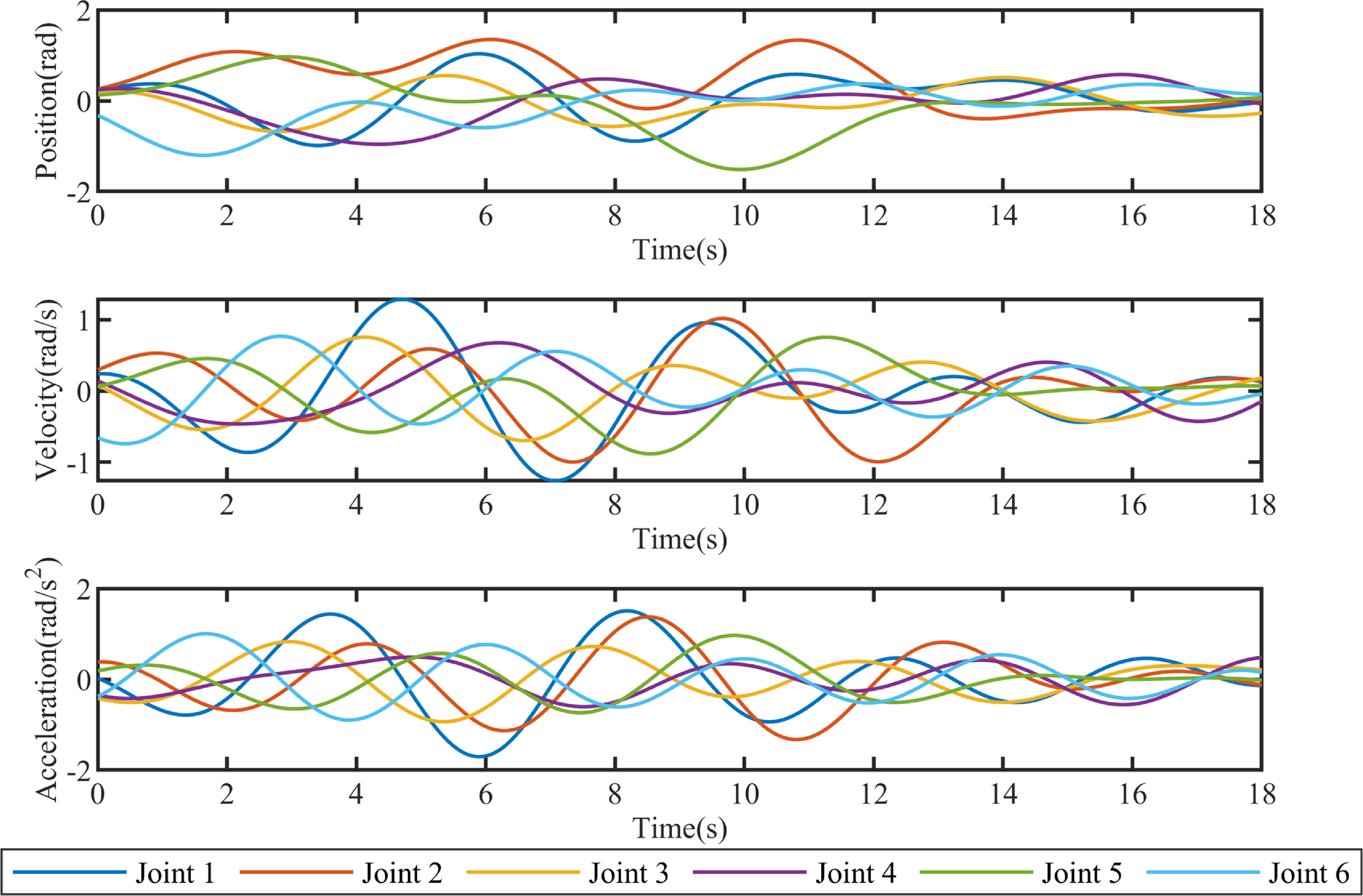
Figure 4. Trajectories used for identifying dynamic parameters.
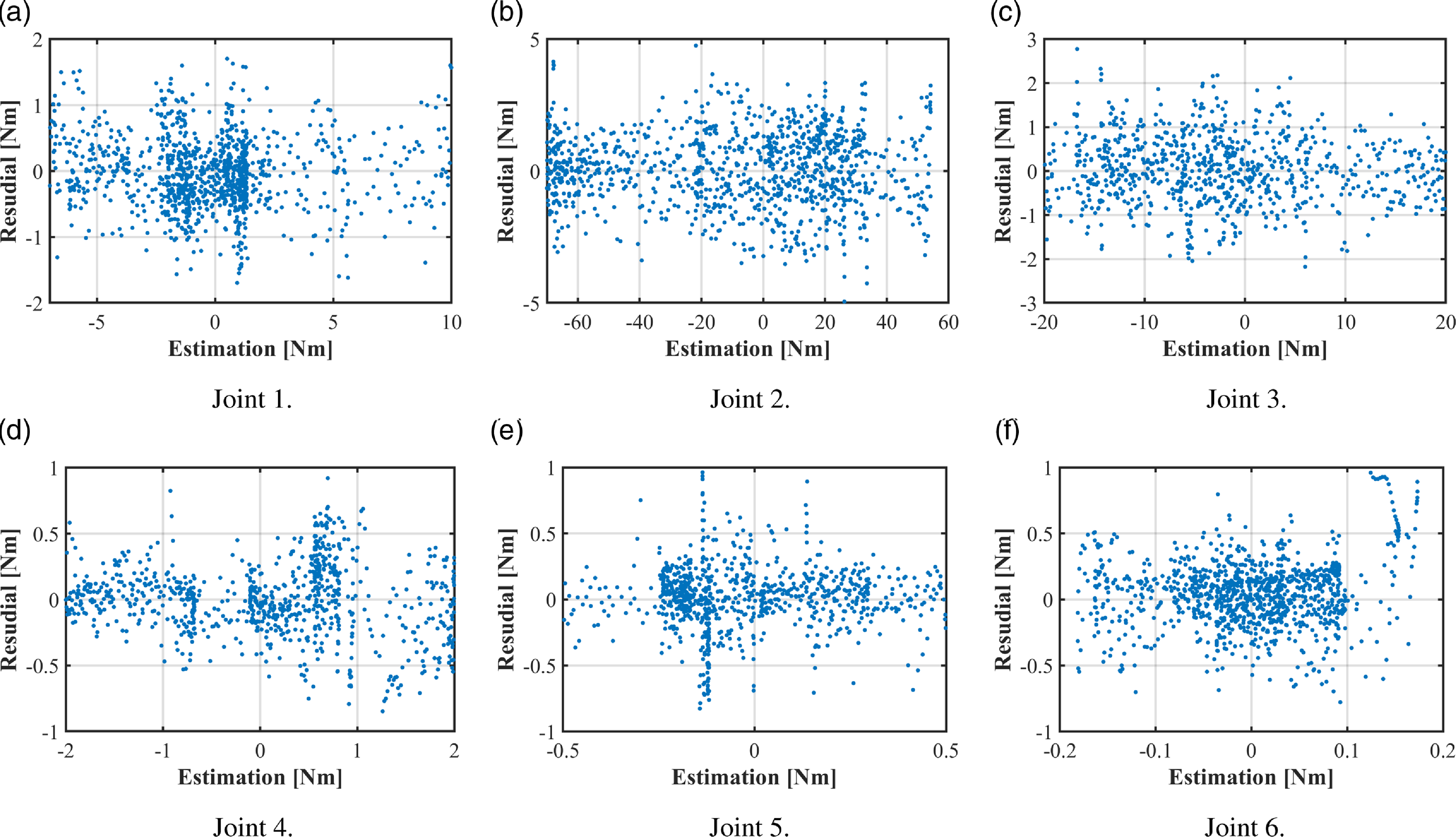
Figure 5. The distribution of residuals vs the fitted values of joint torque.
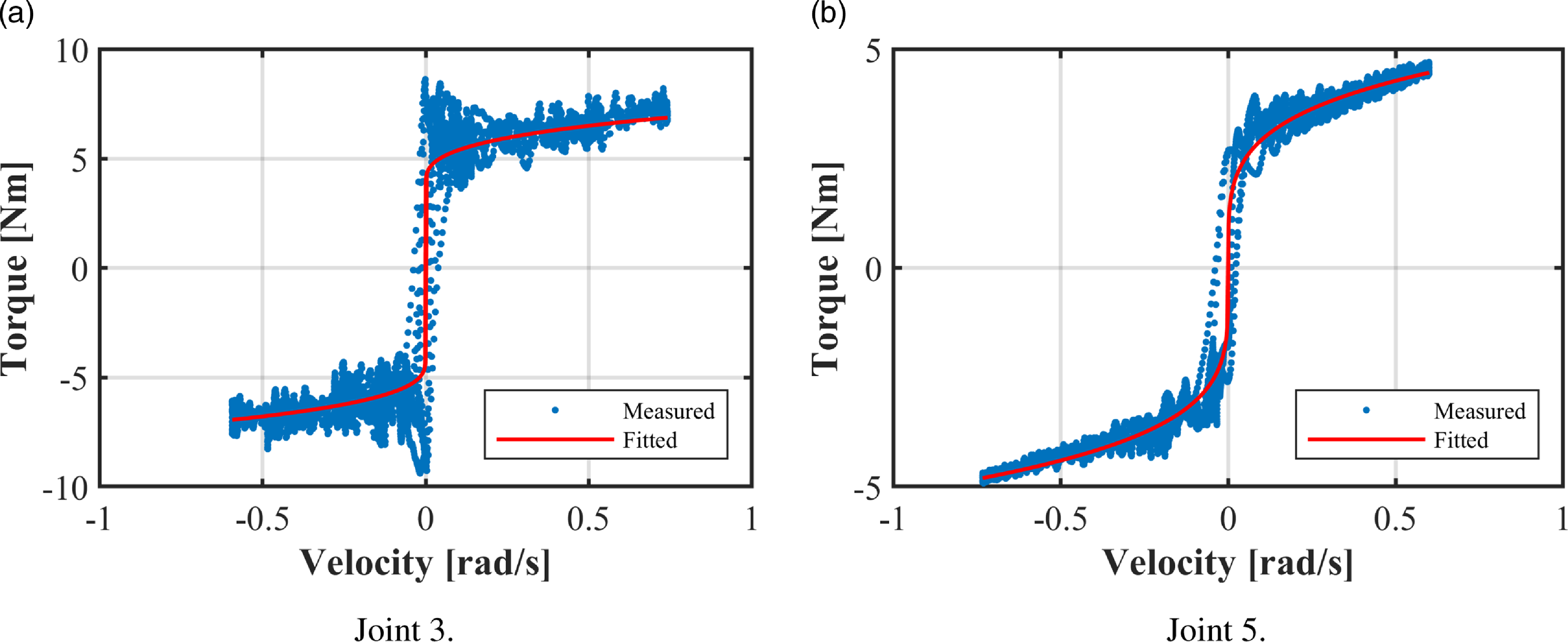
Figure 6. The measured data vs the fitted values of joint friction torque.
Assumption 2.
Independence of residuals. The residuals $\epsilon$
are uncorrelated with each other.
$\epsilon$
are uncorrelated with each other.
Fig. 7 shows the autocorrelation of residual terms. It is seen that the autocorrelation coefficient of each joint lies within $\pm 0.15$
, which is the same threshold as IRLS, thus indicating the independence assumption of the residuals in I-IRLS remains unchanged [Reference Han, Wu, Liu and Xiong11].
$\pm 0.15$
, which is the same threshold as IRLS, thus indicating the independence assumption of the residuals in I-IRLS remains unchanged [Reference Han, Wu, Liu and Xiong11].

Figure 7. Autocorrelation of normalized residuals. The horizontal axis represents the associated lags of time series while the vertical one denotes the sample’s autocorrelation function. The red and yellow dashed lines stand for the maximum and minimum values of the autocorrelation function excluding the initial moment.
Figure 8. The probability density of the residual values. The horizontal axis denotes the residuals of the dynamic model, and the vertical one represents their probability density functions (PDF). Here, the histogram depicts the PDF, while the solid red line gives the data that is fitted from the empirical standard deviation.

Figure 9. The quantile-quantile plot of residual values. The plot shows the quantiles of the calculated residual values versus the theoretical quantile values from a normal one. The data plot of each joint appears linear, and so the distribution of residuals is normal.
Assumption 3. Constant variance. The variance is the constant residuals and does not depend on the predictor variables.
Fig. 5 also shows that the residuals’ mean value is approximately zero and the residuals are randomly distributed without any pattern. This feature indicates that there is no trend or curvature for the residuals and their predicted values, and so it is verified that the variance of the error is constant.
Assumption 4. Normality. The residuals are normally distributed with the mean value being zero, or approximately so.
Figs. 8 and 9 both reveal that for each joint, the residuals almost have the normal distribution with its mean value being 0. The slight asymmetry of the distribution is caused by the underfitting friction at near-zero velocities demonstrated in Fig. 6. The residuals of the classical identification algorithm are mostly velocity-dependent, and this is caused by the difficulty of accurate modeling on the static friction model [Reference Wahrburg, Bös, Listmann, Dai, Matthias and Ding32]. However, the IRLS-based identification algorithm framework filters the data at near-zero velocities when it eliminates the outliers in the middle-loop iteration. Thus, the interference between the data and the identification is reduced in the near-zero velocity region, and the residuals show an independent normal distribution with a mean value of zero [Reference Han, Wu, Liu and Xiong11]. Additionally, this conclusion also provides a theoretical support to the dynamics-based external force estimation such as the one proposed in [Reference Wahrburg, Bös, Listmann, Dai, Matthias and Ding32].
Assumption 5. Convergence. The identification results converge in each loop.
Figs. 10(a) and 10(b) show that I-IRLS guarantees the convergence of the covariance matrix and the weighted vector as IRLS does. Figs. 10(c) and 10(d) indicate that the residuals of the model decrease and gradually converge in both $L_3$
and
$L_3$
and $L_4$
. Fig. 11 shows the convergence process of model parameters in L3. It deserves noting that the accuracy of the model is significantly improved in the second time as compared with the first one. This is because the priori knowledge of the friction compensation in Eq. (8) and the load moment calculated in Eq. (18) are inaccurate at the beginning. The model parameters gradually converge to the solution of the optimization problem, and as a result, the error of the model is reduced.
$L_4$
. Fig. 11 shows the convergence process of model parameters in L3. It deserves noting that the accuracy of the model is significantly improved in the second time as compared with the first one. This is because the priori knowledge of the friction compensation in Eq. (8) and the load moment calculated in Eq. (18) are inaccurate at the beginning. The model parameters gradually converge to the solution of the optimization problem, and as a result, the error of the model is reduced.

Figure 10. Convergence of the four loops of the identification algorithm.

Figure 11. Convergence of the results of the identification algorithm.
Table II shows the estimated solutions $\hat{\theta }$
, the F-statistic
$\hat{\theta }$
, the F-statistic $\hat{F}_{\hat{\theta }}$
and the relative standard deviations (RSD)
$\hat{F}_{\hat{\theta }}$
and the relative standard deviations (RSD) $\hat{\sigma }_{\hat{\theta }}$
. The values of RSD are computed by using the formula in [Reference Sousa and Cortesão12], and if a parameter’s RSD is large, its estimation would probably be bad. The F-statistic values are obtained through the iterative approach in [Reference Jubien, Gautier and Janot33], and they characterize the contribution of parameters to the robot dynamics. If
$\hat{\sigma }_{\hat{\theta }}$
. The values of RSD are computed by using the formula in [Reference Sousa and Cortesão12], and if a parameter’s RSD is large, its estimation would probably be bad. The F-statistic values are obtained through the iterative approach in [Reference Jubien, Gautier and Janot33], and they characterize the contribution of parameters to the robot dynamics. If $\hat{F}$
is less than the threshold
$\hat{F}$
is less than the threshold $F_d$
=3.85, which is obtained from the Fisher-Snedecor table with
$F_d$
=3.85, which is obtained from the Fisher-Snedecor table with $\alpha$
= 5%, the corresponding parameter will be reduced without any significant effect on the dynamic model.
$\alpha$
= 5%, the corresponding parameter will be reduced without any significant effect on the dynamic model.
Table II. The I-IRLS solution $^{1}$
.
$^{1}$
.
 $^{1}$
All the units are in SI unit.
$^{1}$
All the units are in SI unit. $^{2}$
Only results
$^{2}$
Only results $\hat{F}_{\hat{\theta }} \lt F_d$
are shown.
$\hat{F}_{\hat{\theta }} \lt F_d$
are shown.
Table II indicates that the values of parameters such as $\theta _{27}$
and
$\theta _{27}$
and $\theta _{30}$
, whose RSD is large, are in lower order of magnitude and thus can be removed from the dynamic model. This reveals a characteristic of the IRLS-based algorithm: It improves the accuracy of the dynamic model by reducing the magnitude of the noise-sensitive parameters, and so they hardly affect the estimation results of the dynamic model and can even be ignored in the calculation. This feature also leads to a feasible solution to the computational errors caused by practical parameters of lower order of magnitude.
$\theta _{30}$
, whose RSD is large, are in lower order of magnitude and thus can be removed from the dynamic model. This reveals a characteristic of the IRLS-based algorithm: It improves the accuracy of the dynamic model by reducing the magnitude of the noise-sensitive parameters, and so they hardly affect the estimation results of the dynamic model and can even be ignored in the calculation. This feature also leads to a feasible solution to the computational errors caused by practical parameters of lower order of magnitude.
3.3. Comparison among different identification methods
In this section, the data from a set of excitation trajectories are used to calculate the dynamic parameters, while other 25 sets of trajectories are applied as testing sets to verify the performance of the algorithms. For comparison, six different cases of the proposed I-IRLS are adopted to estimate the model parameters. Three basic models are involved here: Model I does not consider the effect of load on friction, model II adopts the linear load-friction relationship, and model III employs a squared load-friction function as shown in section 2.2 Each model is investigated in two different cases with and without considering the linear temperature-friction function (abbr. as “with” and “without,” for simplicity). When no temperature-friction relationship is taken into account, model I reduces to the classical IRLS.
The predicted results of these models on the testing sets of trajectories are shown in Fig. 12(a), from where the following conclusions can be obtained:
-
(a) In each group, the Root Mean Square Error (RMSE) of the model in the “with” case is smaller than that in the “without” case.
-
(b) When the same temperature-friction function is applied, the model’s RMSE is smaller if a more accurate load-friction relationship is considered.
-
(c) The performances of models II and III are quite close to each other, and their results are not obviously different in a statistical sense. The reason for this phenomenon is that the linear and quadratic load-friction functions are approximately equivalent when the joint load torque is small, as shown in Fig. 2.
The above results indicate that the model that considers the temperature-friction and load-friction effects can significantly improve the identification accuracy. Specifically, the RMSE can be reduced by more than 13%.

Figure 12. RMSE of residuals in cross-validations. The top horizontal bars reflect the statistical significance between the results of the two algorithms and those of I-IRLS.
3.4. Comparison with other supervised identification algorithms
For comparison, three validation trajectories were calculated using the Eqs. (20) and (13), and a test dataset of 20 sets of data were collected to compare and validate the performance of four algorithms: (a) LS, (b) IRLS [Reference Han, Wu, Liu and Xiong11], and (c) I-IRLS, proposed in this research. The RMSE of the prediction results for each algorithm were recorded separately in Fig. 12 (b). For each algorithm, two different histograms are depicted to show the prediction errors in the LS and LMI-SDP cases, respectively. The predicted RMSE of these algorithms on the testing sets of trajectories is shown in Fig. 12(b). The joint running states were categorized into a low-speed state and a high-speed state, according to the relationship between the joint velocity and the boundary of the mixed lubrication interval (i.e., 0.1 [rad/s]) in the Stribeck Curve of joint friction. Tables III and IV present the mean and standard deviation of the maximum estimation error (abbr. as “M” and “STD,” for simplicity) for the three elbow joints (i.e., from the 1st to the 3rd joint) and the three wrist joints (i.e., from the 4th to the 6th joint) on the validation dataset.
From the test results, the following conclusions can be drawn:
-
(a) Comparing LS with other IRLS-based algorithms, one can find that the LS always has the largest RMSE and the largest residual. This is mainly caused by the outliers due to separated compensation of joint friction.
-
(b) When IRLS is compared with the proposed I-IRLS, it is indicated that the RMSE and standard deviation of the maximum error of the I-IRLS algorithm are significantly lower than those of IRLS. The maximum errors of the two algorithms within the low-speed zone of the elbow joints differ by less than 1%. Furthermore, the mean value of the maximum error for the I-IRLS algorithm is significantly lower than that of IRLS. This suggests that incorporating temperature-friction and load-friction factors into the identification algorithms can enhance the accuracy and robustness of the models.
-
(c) The proposed I-IRLS reduces the RMSE by over 14% compared to IRLS and over 16% compared to LS. Additionally, the estimation results of the proposed I-IRLS have the lowest error standard deviation in terms of maximum error. This is particularly evident in the high-speed region of the elbow joint, where the driving torque is high and the temperature variation is significant. In this region, the proposed I-IRLS reduces the error by more than 33% compared to IRLS and by more than 47% compared to LS. In the low-speed region, where temperature changes are not obvious and friction dynamics are more dynamic, I-IRLS shows improvement compared to other algorithms.
-
(d) All identification algorithms show significantly higher fitting errors in the low-speed region than in other regions, which is due to the fact that the IRLS-based identification algorithms identify and filter the data within the low-speed region in the iterations, which reduces the fitting accuracy in this region. Furthermore, the static model used in the recognition algorithm is incapable of ensuring the dynamics of friction within the low-speed region, leading to a decrease in model accuracy within this region, as shown in Fig 6.
-
(e) The histograms for each algorithm show that the RMSE of LMI-SDP is higher than that of LS, indicating that the identification results deviate from the numerical solution of linear regression when physical feasibility constraints are present. However, LMI-SDP has a lower standard deviation in terms of maximum estimation error, demonstrating its high robustness with respect to physical feasibility parameters.
The predicted errors of these algorithms on one cross-validation trajectory are shown in Fig. 13. It is seen that the residual of I-IRLS is generally smaller than that of other algorithms. It deserves noting that the residuals of each algorithm are significantly larger in the near-zero-velocity region than that of other cases. This phenomenon can be improved in I-IRLS by considering a more comprehensive friction model. It also reveals that a more accurate and comprehensive friction modeling and identification are essential for improving dynamic model accuracy.
Table III. Maximum estimation error in identification results of elbow joints $^{[1]}$
.
$^{[1]}$
.
 $^{[1]}$
Joints’ internal temperature increased from 25.5
$^{[1]}$
Joints’ internal temperature increased from 25.5 $^{\circ }$
C to 40.6
$^{\circ }$
C to 40.6 $^{\circ }$
C.
$^{\circ }$
C. $^{[2]}$
Based on LS.
$^{[2]}$
Based on LS. $^{[3]}$
Based on LMI-SDP.
$^{[3]}$
Based on LMI-SDP.
Table IV. Maximum estimation error in identification results of wrist joints $^{1}$
.
$^{1}$
.
 $^{[1]}$
Joints’ internal temperature increased from 26.4
$^{[1]}$
Joints’ internal temperature increased from 26.4 $^{\circ }$
C to 29.5
$^{\circ }$
C to 29.5 $^{\circ }$
C.
$^{\circ }$
C. $^{[2]}$
Based on LS.
$^{[2]}$
Based on LS. $^{[3]}$
Based on LMI-SDP.
$^{[3]}$
Based on LMI-SDP.

Figure 13. Predicted errors of cross-validations.
4. Conclusion
This research aims at developing an accurate, generalized and robust dynamic model identification algorithm for collaborative robots. For this purpose, an improved iterative approach is proposed with a comprehensive friction model for considering the velocity, temperature and load torque effects. Specifically, the iterative approach is put forth to estimate the dynamic model parameters based on the reweighted least-squares algorithm. Besides, the comprehensive friction model is proposed to enhance the accuracy and robustness of the dynamic parameters’ identification model. Experiments verify that: (a) The RMSE of the proposed algorithm is reduced by over 14% than those of other identification algorithms, and (b) the proposed algorithm has better robustness for collaborative robots especially when temperature varies significantly at their joints.
When collaborative robots serve in practical environments, the velocity, temperature and load torque of the joints vary markedly due to the heat-dissipation of motor, ambient temperature change and configural change [Reference Gao, Yuan, Han, Wang and Wang24]. Therefore, the proposed I-IRLS algorithm has wide practical application prospects in compliance control [Reference Hu and Xiong6], collision detection [Reference Haddadin, De Luca and Albu-Schaffer34] and hand-guiding programming [Reference Althoff, Giusti, Liu and Pereira3].
Author contributions
All authors contributed to the study’s conception and design. Material preparation, data collection and analysis were performed by Zeyu Li, Hongxing Wei, Chengguo Liu and Gang Liu. The first draft of the manuscript was written by Zeyu Li and extended by Hongxing Wei, Ye He, Haochen Zhang and Weiming Li. All authors commented on previous versions of the manuscript. All authors read and approved the final manuscript.
Financial support
This work was partially supported by National Key R&D Program of China (2019YFB1309900).
Competing interests
No competing interests.
Ethical approval
None.
Appendix: Symbolic Expressions of the Minimum Parameter Set for AUBO I5
 \begin{equation}{\theta _1} = a_3^2\sum \limits _{i = 3}^6{{m_i}} + d_2^2\sum \limits _{i = 2}^6{{m_i}} + a_4^2\sum \limits _{i = 4}^6{{m_i}} + 2{d_2}\sum \limits _{i = 2}^4{{S_{z,i}}} + \sum \limits _{i = 2}^4{{I_{yy,i}}} +{I_{zz,1}} \end{equation}
 \begin{equation}{\theta _2} ={f_{c,1}} \end{equation}
 \begin{equation}{\theta _3} ={f_{v,1}} \end{equation}
 \begin{equation}{\theta _4} ={f_{o,1}} \end{equation}
 \begin{equation}{\theta _5} = - a_3^2\sum \limits _{i = 3}^6{{m_i}} +{I_{xx,2}} -{I_{yy,2}} \end{equation}
 \begin{equation}{\theta _6} ={I_{xy,2}} \end{equation}
 \begin{equation}{\theta _7} ={a_3}S_{z,3}-{a_3}S_{z,4} +{I_{xz,2}} \end{equation}
 \begin{equation}{\theta _8} ={I_{yz,2}} \end{equation}
 \begin{equation}{\theta _9} = a_3^2\sum \limits _{i = 3}^6{{m_i}} +{I_{zz,2}} \end{equation}
 \begin{equation}{\theta _{10}} ={a_3}\sum \limits _{i = 3}^6{{m_i}} +{S_{x,2}} \end{equation}
 \begin{equation}{\theta _{11}} ={S_{y,2}} \end{equation}
 \begin{equation}{\theta _{12}} ={f_{c,2}} \end{equation}
 \begin{equation}{\theta _{13}} ={f_{v,2}} \end{equation}
 \begin{equation}{\theta _{14}} ={f_{o,2}} \end{equation}
 \begin{equation}{\theta _{15}} = - a_4^2\sum \limits _{i = 4}^6{{m_i}} +{I_{xx,3}} -{I_{yy,3}} \end{equation}
 \begin{equation}{\theta _{16}} ={I_{xy,3}} \end{equation}
 \begin{equation}{\theta _{17}} ={a_4}{S_{z,4}} +{I_{xz,3}} \end{equation}
 \begin{equation}{\theta _{18}} ={I_{yz,3}} \end{equation}
 \begin{equation}{\theta _{19}} = a_4^2\sum \limits _{i = 4}^6{{m_i}} +{I_{zz,3}} \end{equation}
 \begin{equation}{\theta _{20}} ={a_4}\sum \limits _{i = 4}^6{{m_i}} +{S_{x,3}} \end{equation}
 \begin{equation}{\theta _{21}} ={S_{y,3}} \end{equation}
 \begin{equation}{\theta _{22}} ={f_{c,3}} \end{equation}
 \begin{equation}{\theta _{23}} ={f_{v,3}} \end{equation}
 \begin{equation}{\theta _{24}} ={f_{o,3}} \end{equation}
 \begin{equation}{\theta _{25}} ={d_5}\sum \limits _{i = 5}^6{{m_i}} + 2{d_5}{S_{z,5}} +{I_{xx,4}} -{I_{yy,4}} +{I_{yy,5}} \end{equation}
 \begin{equation}{\theta _{26}} ={I_{xy,4}} \end{equation}
 \begin{equation}{\theta _{27}} ={I_{xz,4}} \end{equation}
 \begin{equation}{\theta _{28}} ={I_{yz,4}} \end{equation}
 \begin{equation}{\theta _{29}} = d_5^2\sum \limits _{i = 5}^6{{m_i}} + 2{d_5}{S_{z,5}} +{I_{zz,4}} +{I_{yy,5}} \end{equation}
 \begin{equation}{\theta _{30}} ={S_{x,4}} \end{equation}
 \begin{equation}{\theta _{31}} ={d_5}\sum \limits _{i = 5}^6{{m_i}} +{S_{y,4}} +{S_{z,5}} \end{equation}
 \begin{equation}{\theta _{32}} ={f_{c,4}} \end{equation}
 \begin{equation}{\theta _{33}} ={f_{v,4}} \end{equation}
 \begin{equation}{\theta _{34}} ={f_{o,4}} \end{equation}
 \begin{equation}{\theta _{35}} ={d_6}{m_6} + 2{d_6}{S_{z,6}} +{I_{xx,5}} -{I_{yy,5}} +{I_{yy,6}} \end{equation}
 \begin{equation}{\theta _{36}} ={I_{xy,5}} \end{equation}
 \begin{equation}{\theta _{37}} ={I_{xz,5}} \end{equation}
 \begin{equation}{\theta _{38}} ={I_{yz,5}} \end{equation}
 \begin{equation}{\theta _{39}} = d_6^2{m_6} + 2{d_6}{S_{z,6}} +{I_{zz,5}} +{I_{yy,6}} \end{equation}
 \begin{equation}{\theta _{40}} ={S_{x,5}} \end{equation}
 \begin{equation}{\theta _{41}} = -{d_6}{m_6} -{S_{z,6}} +{S_{y,5}} \end{equation}
 \begin{equation}{\theta _{42}} ={f_{c,5}} \end{equation}
 \begin{equation}{\theta _{43}} ={f_{v,5}} \end{equation}
 \begin{equation}{\theta _{44}} ={f_{o,5}} \end{equation}
 \begin{equation}{\theta _{45}} ={I_{xx,6}} -{I_{yy,6}} \end{equation}
 \begin{equation}{\theta _{46}} ={I_{xy,6}} \end{equation}
 \begin{equation}{\theta _{47}} ={I_{xz,6}} \end{equation}
 \begin{equation}{\theta _{48}} ={I_{yz,6}} \end{equation}
 \begin{equation}{\theta _{49}} ={I_{zz,6}} \end{equation}
 \begin{equation}{\theta _{50}} ={S_{x,6}} \end{equation}
 \begin{equation}{\theta _{51}} ={S_{y,6}} \end{equation}
 \begin{equation}{\theta _{52}} ={f_{c,6}} \end{equation}
 \begin{equation}{\theta _{53}} ={f_{v,6}} \end{equation}
 \begin{equation}{\theta _{54}} ={f_{o,6}} \end{equation}
where $a$
and
$a$
and $d$
are D-H parameters provided in Table I.
$d$
are D-H parameters provided in Table I.


