2.1. Problem description

The continuum robot is generally composed of several segments and each segment is driven by four cables [Reference Zheng, Ding, Liu, Zhu and Guo38]. The spring deforms elastically by pulling the actuated cables, resulting in flexible bending of the robot. The spacer disks are evenly spaced and the adjacent spacer disks are connected by universal joints. Figure 1 shows a two-segment cable-driven continuum robot prototype model.

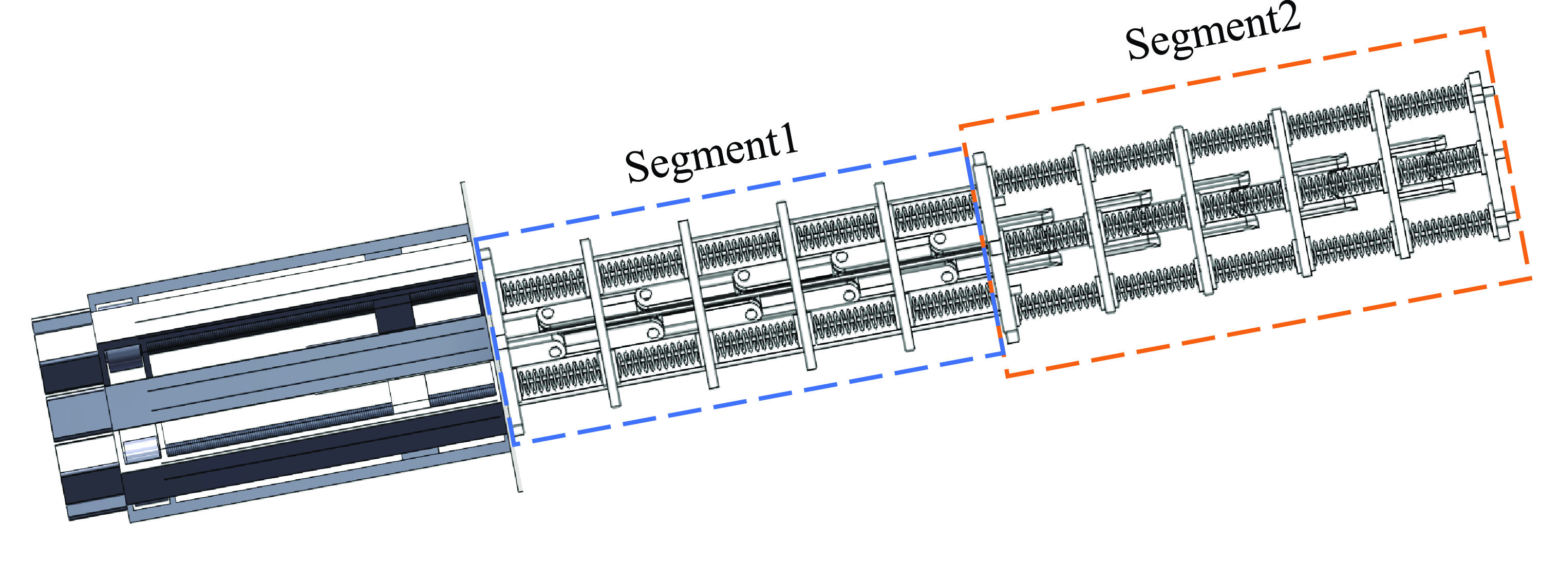
Figure 1. A two-segment cable-driven continuum robot prototype.

The goal of path planning for the continuum robot is that a continuous path needs to be found between the initial state and the target state in the constrained workspace. Figure 2 shows the operation of a two-segment continuum robot in the task space with three obstacles from the starting point ‘S’ to the end target point ‘E’. The Cartesian coordinate ${O_1} -{X_1}{Y_1}{Z_1}$ is the base coordinate frame of the continuum robot system. ${O_2} -{X_2}{Y_2}{Z_2}$ and ${O_3} -{X_3}{Y_3}{Z_3}$ represent the coordinate frame of the end the spacer disk for the first-segment and second-segment continuum robot respectively. This work aims to find a feasible path that avoids obstacles and satisfies the physical constraints of the continuum robot while considering the efficiency and accuracy in performing tasks.

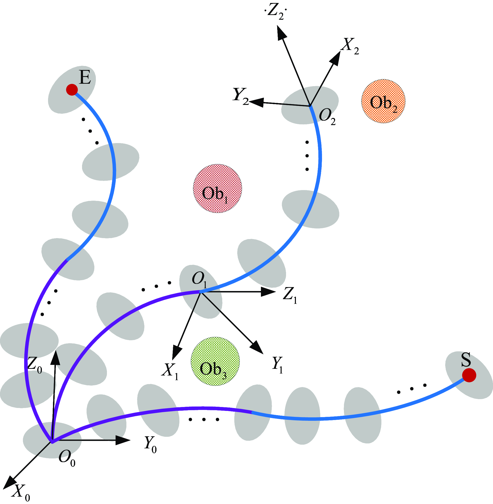
Figure 2. Continuum robot path planning in the obstacle environment.

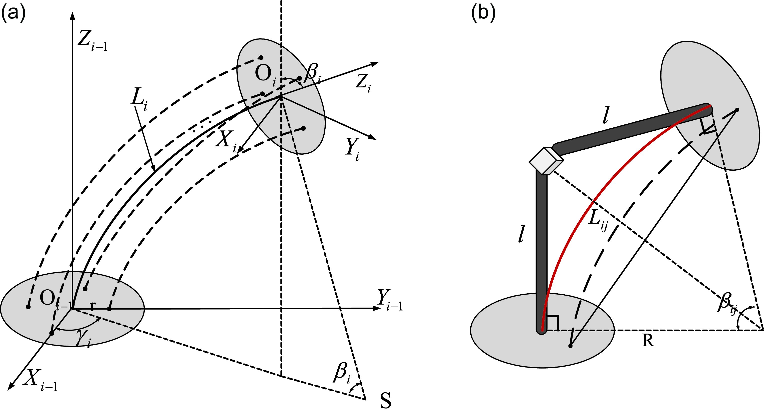
Figure 3. (a) Coordinate frame schematic of the ith-segment continuum robot and (b) bending schematic of the adjacent spacer plates.

2.2. Kinematic model

The kinematics model of the $N$ -segment continuum robot model is established in this section. Due to the small spacing between adjacent disks, the elastic deformation produced by springs with the same specifications under the approximate force is also approximately equal. Thus, it is assumed that each segment of the continuum robot acts like a constant curvature arc. For the $i$ th-segment, the coordinate frame schematic is illustrated in Fig. 3 (a). Each segment of the continuum robot can be parameterized by two variables $\beta _i$ and $\gamma _i$ in the configuration space, where $\beta _i$ represents the bending angle and $\gamma _i$ is rotation angle around the axis $Z_{i - 1}$ respectively. The arc length of the $i$ th-segment is denoted by $L_i$ . Based on the assumption of constant curvature, the bending angles of the adjacent spacer disks in the same segment are equal. As shown in Fig. 3 (b), the bending angle of $j$ th adjacent spacer disk is defined as $\beta _{ij}$ and the distance between them is 2 $l$ . According to the geometric relationship, the arc length $L_{ij}$ can be calculated by

(1) \begin{equation} {L_{ij}} ={\beta _{ij}}R \end{equation}

where $R$ is the arc radius. In addition, it is easy to obtain the relationship between $R$ and $l$ .

(2) \begin{equation} l = R\tan\! \left ({\frac{{{\beta _{ij}}}}{2}} \right ) \end{equation}

Thus, the arc length $L_i$ is given by

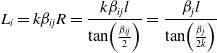(3) \begin{equation} {L_i} = k{\beta _{ij}}R = \frac{{k{\beta _{ij}}l}}{{\tan\! \left ({\frac{{{\beta _{ij}}}}{2}} \right )}} = \frac{{{\beta _j}l}}{{\tan\! \left ({\frac{{{\beta _j}}}{{2k}}} \right )}} \end{equation}

where $k$ is the number of the spacer disks in the $i$ th-segment.

The transformation matrix for the $i$ th-segment is presented as [Reference Webster and Jones39]

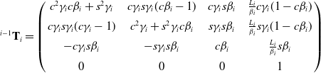(4) \begin{equation} {}^{i - 1}{{\textbf{T}}_i} = \left ({\begin{array}{c@{\quad}c@{\quad}c@{\quad}c}{{c^2}{\gamma _i}c{\beta _i} +{s^2}{\gamma _i}}&{c{\gamma _i}s{\gamma _i}(c{\beta _i} - 1)}&{c{\gamma _i}s{\beta _i}}&{\frac{{{L_i}}}{{{\beta _i}}}c{\gamma _i}(1 - c{\beta _i})}\\[5pt] {c{\gamma _i}s{\gamma _i}(c{\gamma _i} - 1)}&{{c^2}{\gamma _i} +{s^2}{\gamma _i}c{\beta _i}}&{s{\gamma _i}s{\beta _i}}&{\frac{{{L_i}}}{{{\beta _i}}}s{\gamma _i}(1 - c{\beta _i})}\\[5pt] { - c{\gamma _i}s{\beta _i}}&{ - s{\gamma _i}s{\beta _i}}&{c{\beta _i}}&{\frac{{{L_i}}}{{{\beta _i}}}s{\beta _i}}\\[5pt] 0&0&0&1 \end{array}} \right ) \end{equation}

where ${\mathrm{c}}{\beta _i}$ , ${\mathrm{c}}{\gamma _i}$ , ${\mathrm{s}}{\beta _i}$ , ${\mathrm{s}}{\gamma _i}$ stand for the abbreviation of function $\cos{\beta _i}$ , $\cos{\gamma _i}$ , $\sin{\beta _i}$ , $\sin{\gamma _i}$ respectively.

The kinematic mapping relationship for the $N$ -segment continuum robot can be expressed as

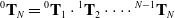(5) \begin{equation} {}^0{{\textbf{T}}_N} ={}^0{{\textbf{T}}_1} \cdot{}^1{{\textbf{T}}_2} \cdots \cdot{}^{N - 1}{{\textbf{T}}_N} \end{equation}

Since the actuated cables remain taut between the spacers as seen from Fig. 3 (b), the length variation of the actuated cables $\Delta{l_{i,m}}$ ( $m$ = 1, 2, 3, 4) can be expressed as

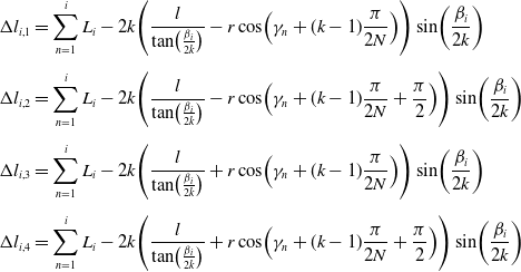(6) \begin{align} \Delta{l_{i,1}} &= \sum \limits _{n = 1}^i{{L_i} - 2k\!\left ({\frac{l}{{\tan\! \left ({\frac{{{\beta _i}}}{{2k}}} \right )}} - r\cos\! \left ({{\gamma _n} + (k - 1)\frac{\pi }{{2N}}} \right )} \right )} \sin\! \left ({\frac{{{\beta _i}}}{{2k}}} \right )\nonumber \\[5pt] \Delta{l_{i,2}} &= \sum \limits _{n = 1}^i{{L_i} - 2k\!\left ({\frac{l}{{\tan\! \left ({\frac{{{\beta _i}}}{{2k}}} \right )}} - r\cos\! \left ({{\gamma _n} + (k - 1)\frac{\pi }{{2N}} + \frac{\pi }{2}} \right )} \right )} \sin\! \left ({\frac{{{\beta _i}}}{{2k}}} \right )\nonumber \\[5pt] \Delta{l_{i,3}} &= \sum \limits _{n = 1}^i{{L_i} - 2k\!\left ({\frac{l}{{\tan\! \left ({\frac{{{\beta _i}}}{{2k}}} \right )}} + r\cos\! \left ({{\gamma _n} + (k - 1)\frac{\pi }{{2N}}} \right )} \right )} \sin\! \left ({\frac{{{\beta _i}}}{{2k}}} \right )\\[5pt] \Delta{l_{i,4}} &= \sum \limits _{n = 1}^i{{L_i} - 2k\!\left ({\frac{l}{{\tan\! \left ({\frac{{{\beta _i}}}{{2k}}} \right )}} + r\cos\! \left ({{\gamma _n} + (k - 1)\frac{\pi }{{2N}} + \frac{\pi }{2}} \right )} \right )} \sin\! \left ({\frac{{{\beta _i}}}{{2k}}} \right )\nonumber \end{align}

Where $r$ is the distance between the cable hole and center hole on the spacer disks.

Remark 1. As shown in Eq. (4), there exists a singular problem when $\beta _i$ is equal to 0. Thus, the fifth-order Taylor expansions of $\cos{{\beta _i}}$ and $\sin{{\beta _i}}$ with respect to $\beta _i$ are applied to avoid singularities, shown as follows:

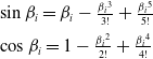(7) \begin{equation} \begin{array}{l} \sin{{\beta _i}} ={\beta _i} - \frac{{{\beta _i}^3}}{{3!}} + \frac{{{\beta _i}^5}}{{5!}}\\[5pt] \cos{{\beta _i}} = 1 - \frac{{{\beta _i}^2}}{{2!}} + \frac{{{\beta _i}^4}}{{4!}} \end{array} \end{equation}

2.3. Collision detection

For the collision detection techniques of the traditional rigid link manipulators, the links are generally equivalent to cylinders, and the minimum distance between the central axis and the obstacle needs to be measured to determine whether the manipulator collides with the obstacle [Reference Menasri, Nakib, Daachi, Oulhadj and Siarry40]. Since the bending direction of the cable-driven continuum robot is not always fixed during the movement and the spacer disks increase the radial distance of the robot body, the robot cannot be simply regarded as an arc in collision detection.

Figure 4. Collision detection model.

Inspired by the collision detection technique of the rigid link manipulators, each segment of the continuum robot is simplified with a curved tubular model in Fig. 4. In order to further simplify the collision detection model, the radial radius of the tubular model is superimposed on the obstacle ball bounding box, where $D$ represents the radius of the ball bounding box and $d$ is the radius of the tubular model. Then the center points ${p_{ij}}\!\left ({j = 1,2, \cdots,k} \right )$ of the spacer disks of the $i$ th-segment are defined as control points which are used to measure the distances ${d_{ij}}\!\left ({j = 1,2, \cdots,k} \right )$ between them and the center of obstacle Q. The minimum distance from the obstacle for the $i$ th-segment $d_i$ can be expressed as

(8) \begin{equation} {d_i} = \min \!\left \{{{d_{ij}}} \right \},j = 1,2, \cdots,k \end{equation}

Therefore, if the minimum distance ${d_i}\!\left ({i = 1,2 \cdots,N} \right )$ satisfies ${d_i} \gt D + d$ , it can be considered that the continuum robot will not collide with the obstacle.

3.1. BAS-APF algorithm

As is shown in Eq. (9), the basic concept of path planning based on APF is to construct a virtual potential field $\boldsymbol{U}$ in the motion space of the robot, where the attraction potential field ${\boldsymbol{U}}_{\mathrm{att}}$ attracts the robot to move toward the target position and the repulsion potential field ${\boldsymbol{U}}_{\mathrm{rep}}$ excludes the robot from obstacles.

(9) \begin{equation} {\boldsymbol{U}} ={{\boldsymbol{U}}_{\mathrm{att}}} +{{\boldsymbol{U}}_{\mathrm{rep}}} \end{equation}

Gradient descent method is usually used to deal with the optimization problem shown in Eq. (9), so as to obtain the joint angle of the robot under the global minimum potential field ${\boldsymbol{U}}_{\min }$ . However, for the case that the working environment of robot is complicated, the drawback that restricts the gradient descent algorithm is the possible existence of local minima in the potential field, where the attraction and repulsion forces are equal in magnitude and opposite in direction.

BAS algorithm imitates the foraging behavior of beetle, using its antennae to search and turn to the direction with stronger smell. The beetle measures the odor concentration at each step to obtain the direction of the next step until it reaches the endpoint, instead of moving randomly in any direction. Inspired by the biological behavior, APF method can be combined with BAS algorithm to handle the problem of local optimization. Figure 5 shows the process of obstacle avoidance path planning based on BAS-APF algorithm, where specially presents how to avoid local optimum.

Figure 5. The path planning process of the BAS-APF algorithm.

This paper constructs a potential field model in the task space and the potential field functions are given considering the special configuration of the continuum robot. The attraction potential field is expressed as

(10) \begin{equation} {{\boldsymbol{U}}_{\mathrm{att}}} = \left \{{\begin{array}{*{20}{c}}{{k_{\mathrm{a}}} \cdot{{\left \|{{\boldsymbol{P}}\!\left ({\boldsymbol{\varphi }} \right ) -{{\boldsymbol{P}}_{\mathrm{ta}}}} \right \|}^2}}&{,\left \|{{\boldsymbol{P}}\!\left ({\boldsymbol{\varphi }} \right ) -{{\textbf{P}}_{\mathrm{ta}}}} \right \| \le{d_{\mathrm{att}}}}\\[5pt] {{k_{\mathrm{a}}} \cdot \left \|{{\boldsymbol{P}}\!\left ({\boldsymbol{\varphi }} \right ) -{{\boldsymbol{P}}_{\mathrm{ta}}}} \right \|}&{,\left \|{{\boldsymbol{P}}\!\left ({\boldsymbol{\varphi }} \right ) -{{\boldsymbol{P}}_{\mathrm{ta}}}} \right \| \gt{d_{\mathrm{att}}}} \end{array}} \right. \end{equation}

where ${\boldsymbol{\varphi }} ={\left [{{\beta _1},{\gamma _1},{\beta _2},{\gamma _2}, \cdots,{\beta _N},{\gamma _N}} \right ]^{\mathrm{T}}}$ is defined as the attitude angle vector of the $N$ -segment continuum robot, $k_{\mathrm{a}}$ is the attractive proportional gain, ${\boldsymbol{P}}\!\left ({\boldsymbol{\varphi }} \right )$ represents the current position of the end-effector, ${\boldsymbol{P}}_{\mathrm{ta}}$ represents the target position, $\left \|{{\boldsymbol{P}}\!\left ({\boldsymbol{\varphi }} \right ) -{{\textbf{P}}_{\mathrm{ta}}}} \right \|$ represents the European distance between the two points, $d_{\mathrm{att}}$ is the set distance threshold.

The repulsion potential field is expressed as

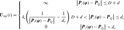(11) \begin{equation} {{\boldsymbol{U}}_{\mathrm{rep}}}\!\left ( i \right ) = \left \{{\begin{array}{*{20}{c}} \infty &{\left \|{{{\boldsymbol{P}}_i}\!\left ({\boldsymbol{\varphi }} \right ) -{{\boldsymbol{P}}_{\mathrm{Q}}}} \right \| \le D + d}\\[9pt] {{k_{\mathrm{r}}}\!\left(\dfrac{1}{{\!\left \|{{{\boldsymbol{P}}_i}\!\left ({\boldsymbol{\varphi }} \right ) -{{\boldsymbol{P}}_{\mathrm{Q}}}} \right \|}} - \dfrac{1}{{{d_o}}}\right)}&{D + d \lt \left \|{{{\boldsymbol{P}}_i}\!\left ({\boldsymbol{\varphi }} \right ) -{{\boldsymbol{P}}_{\mathrm{Q}}}} \right \| \le{d_o}}\\[9pt] 0&{\left \|{{{\boldsymbol{P}}_i}\!\left ({\boldsymbol{\varphi }} \right ) -{{\boldsymbol{P}}_{\mathrm{Q}}}} \right \| \gt{d_o}} \end{array}} \right. \end{equation}

(12) \begin{equation} {{\boldsymbol{U}}_{\mathrm{rep}}} = \sum \limits _{i = 1}^K{{{\boldsymbol{U}}_{\mathrm{rep}}}\!\left ( i \right )} \end{equation}

where $k_{\mathrm{r}}$ is the repulsive proportional gain, ${{\boldsymbol{P}}_i}\!\left ({\boldsymbol{\varphi }} \right )$ represents the position of the $i$ th spacer disk, ${\boldsymbol{P}}_{\mathrm{Q}}$ represents the position of the center of obstacle Q, $\left \|{{{\boldsymbol{P}}_i}\!\left ({\boldsymbol{\varphi }} \right ) -{{\boldsymbol{P}}_{\mathrm{Q}}}} \right \|$ represents the European distance between the two points, $d_o$ is the influence range of the repulsion potential field, the total number of the spacer disks $K$ is calculated as $K = N \cdot k$ .

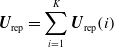
Algorithm 1. BAS-APF algorithm – collision-free path planning

For the cable-driven continuum robot, the computational complexity of the inverse kinematics increases rapidly as the number of segments increase. Meanwhile, the existence of multiple inverse solutions may cause the discontinuity of the planned attitude angle. In this paper, the proposed BAS-APF method mainly uses BAS algorithm to search in the configuration space until the corresponding attitude angle under the minimum potential field is found. Algorithm 1 shows the pseudocode for collision-free path planning. The main flow of path planning for continuum robot is introduced as follows:

1. 1. The attitudes of both directions for the searching antennae at time step t can be presented as

   (13) \begin{equation} \left \{{\begin{array}{*{20}{c}}{{\boldsymbol{\varphi }}_t^{\mathrm{L}} ={{\boldsymbol{\varphi }}_t} +{\lambda _t}\vec{\boldsymbol{b}}}\\[5pt] {{\boldsymbol{\varphi }}_t^{\mathrm{R}} ={{\boldsymbol{\varphi }}_t} -{\lambda _t}\vec{\boldsymbol{b}}} \end{array}} \right. \end{equation}
   (14) \begin{equation} \vec{\boldsymbol{b}} = \frac{{{\mathrm{rnd}}\left ({2N,1} \right )}}{{\left \|{{\mathrm{rnd}}\left ({2N,1} \right )} \right \|}} \end{equation}
   where ${\boldsymbol{\varphi }}_t^{\mathrm{L}}$ and ${\boldsymbol{\varphi }}_t^{\mathrm{R}}$ denote the attitude positions of left and right antennae in the searching area respectively, ${\boldsymbol{\varphi }}_t$ denotes the attitude angle vector at time step $t$ , $\lambda _t$ is the exploration step size of the antenna, $\boldsymbol{\vec b}$ is a normalized random direction vector.

2. 2. Calculate the minimum distance between each segment and obstacles, and then conduct collision detection with Eq. (8). Considering the constraint of obstacles and limitation of attitude angle, the constraint function of attitude angle $\Lambda \!\left ({{\boldsymbol{\varphi }}_t^x} \right )$ can be defined as

   (15) \begin{equation} \begin{array}{l} \Lambda \!\left ({{\boldsymbol{\varphi }}_t^x} \right ) = \left \{{\begin{array}{*{20}{c}}{\max \!\left \{{{{\boldsymbol{\varphi }}_{\min }},\min \!\left \{{{\boldsymbol{\varphi }}_t^x,{{\boldsymbol{\varphi }}_{\max }}} \right \}} \right \}}&{\begin{array}{*{20}{c}}{if}&{{d_i} \gt D + d} \end{array}}\\[5pt] {{{\boldsymbol{\varphi }}_t}}&{\begin{array}{*{20}{c}}{if}&{{d_i} \le D + d} \end{array}} \end{array}} \right .\\[5pt] \begin{array}{*{20}{c}}{}&{}&{}&{}&{}&{}&{}&{}&{}&{}&{}&{}&{}&{}&{}&{}&{}&{}&{}&{} \end{array}i = 1,2, \cdots,N \end{array} \end{equation}
   where $x \in \left \{{{\mathrm{L}},{\mathrm{R}}} \right \}$ , ${\boldsymbol{\varphi }}_{\min }$ and ${\boldsymbol{\varphi }}_{\max }$ are the lower and upper attitude angle limits respectively.

3. 3. The constraint attitude angle is recorded as ${\bar{\boldsymbol \varphi }}_t^x\!\left ({x \in \!\left \{{{\mathrm{L}},{\mathrm{R}}} \right \}} \right )$ according to the constraint function (15). Then the potential fields ${\boldsymbol{U}}\!\left ({{\bar{\boldsymbol \varphi }}_t^x} \right )$ at the positions of the current antenna are calculated combined with Eqs. (9)–(12).

4. 4. Update the next moving direction of the beetle along the descending direction of the potential field, the update rule is given as

   (16) \begin{equation} {\bar{\boldsymbol \varphi }}_t^{'x} = \Lambda \!\left ({{{\boldsymbol{\varphi }}_t} -{\delta _t}\vec{\boldsymbol{b}}{\mathop{\mathrm sgn}} \left ({{\boldsymbol{U}}\left ({{\bar{\boldsymbol \varphi }}_t^{\mathrm{L}}} \right ) -{\boldsymbol{U}}\left ({{\bar{\boldsymbol \varphi }}_t^{\mathrm{R}}} \right )} \right )} \right ) \end{equation}
   Where ${\bar{\boldsymbol \varphi }}_t^{'x}$ is the updated attitude angle, $\delta _t$ donates the updating step size of the antenna, ${\mathop{\mathrm sgn}} \left ( \cdot \right )$ donates the signum function.

5. 5. Calculate the potential field ${\boldsymbol{U}}\left ({{\bar{\boldsymbol \varphi }}_t^{'x}} \right )$ at the position of the updated attitude angle and compared it with the potential field ${\boldsymbol{U}}\left ({{{\boldsymbol{\varphi }}_t}} \right )$ at time step t. If the updated potential field is smaller than that at time step t, the antenna will transfer to the new position. Otherwise, it will remain in the previous position. The attitude angle for the searching antennae at time step $t + 1$ is shown as

   (17) \begin{equation} {{\boldsymbol{\varphi }}_{t + 1}} = \left \{{\begin{array}{*{20}{c}}{{\bar{\boldsymbol \varphi }}_t^{'x}}\\[5pt] {{{\boldsymbol{\varphi }}_t}} \end{array}\begin{array}{*{20}{c}}{}\\[5pt] {} \end{array}\begin{array}{*{20}{c}}{if}&{{\boldsymbol{U}}\left ({{\bar{\boldsymbol \varphi }}_t^{'x}} \right ) \lt{\boldsymbol{U}}\left ({{{\boldsymbol{\varphi }}_t}} \right )}\\[5pt] {if}&{{\boldsymbol{U}}\left ({{\bar{\boldsymbol \varphi }}_t^{'x}} \right ) \ge{\boldsymbol{U}}\left ({{{\boldsymbol{\varphi }}_t}} \right )} \end{array}} \right. \end{equation}

6. 6. After moving to the new position, return to step 1 and enter the next searching cycle until reaching the neighborhood range $r_{{\mathrm{th}}}$ of target point. If the cycle ends at time step $t_{\mathrm{max}}$ and the target position has not been reached, the beetle is considered to be trapped in the local optimum. Then turn back to the previous position at time step $t_{\mathrm{max}-1}$ and reenter to Step 1 for a new searching cycle.

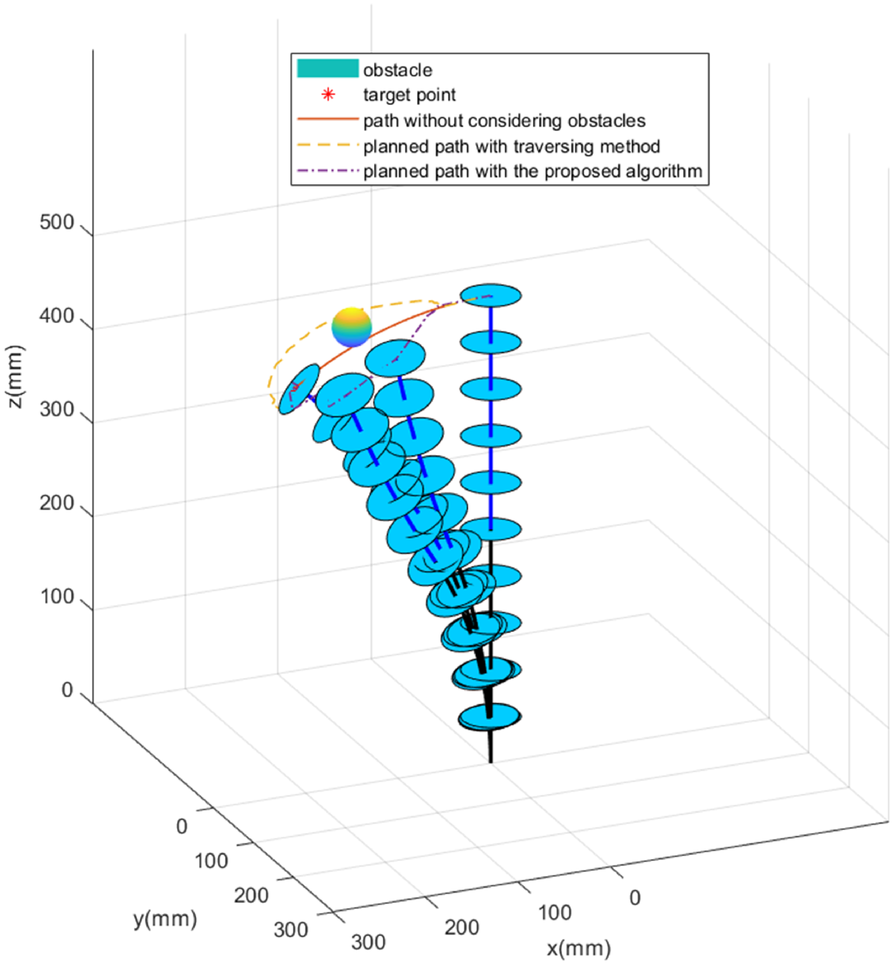
Figure 6. Path planning in the single obstacle environment.

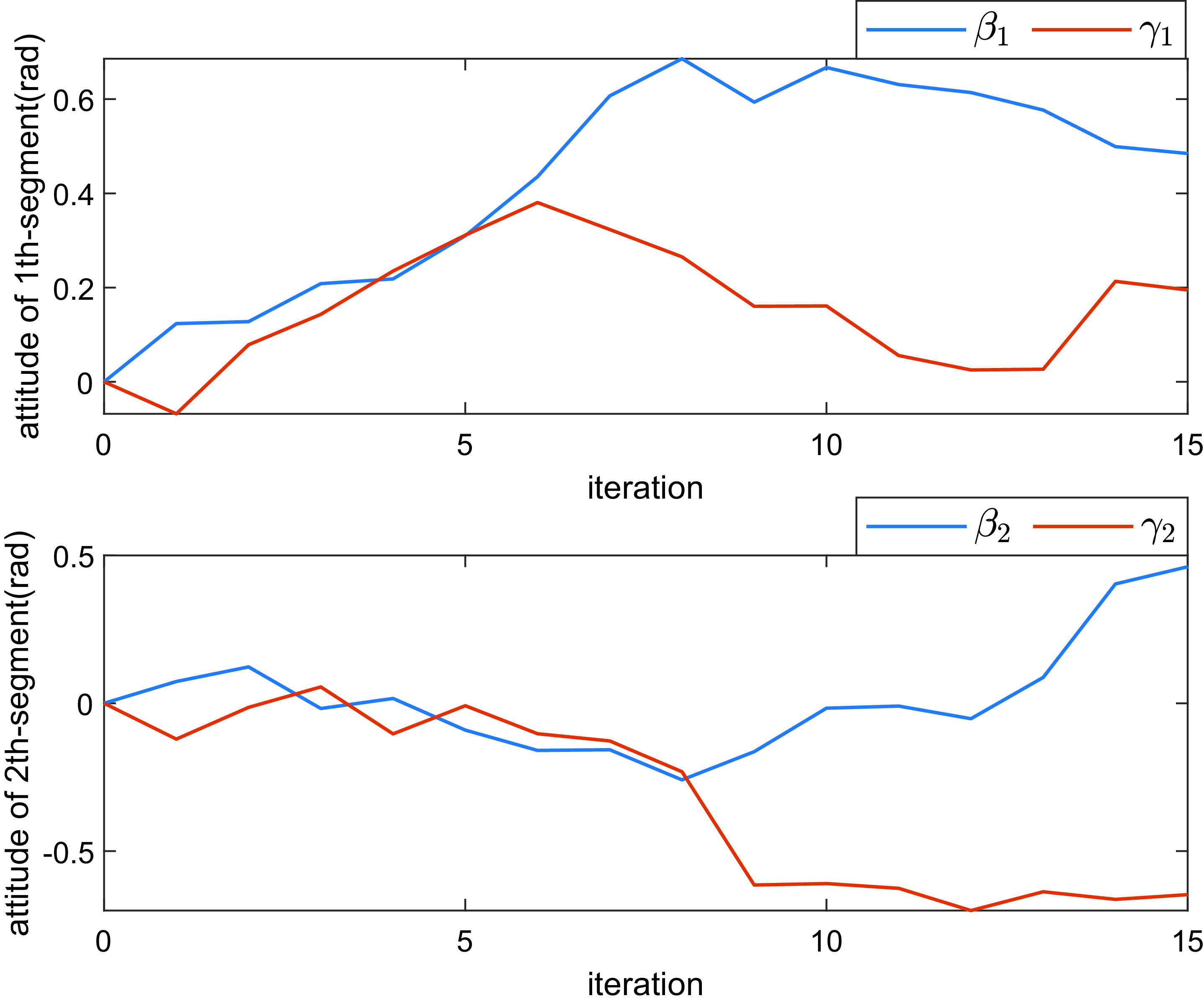
Figure 7. Attitude angle curve for the obstacle avoidance planning.

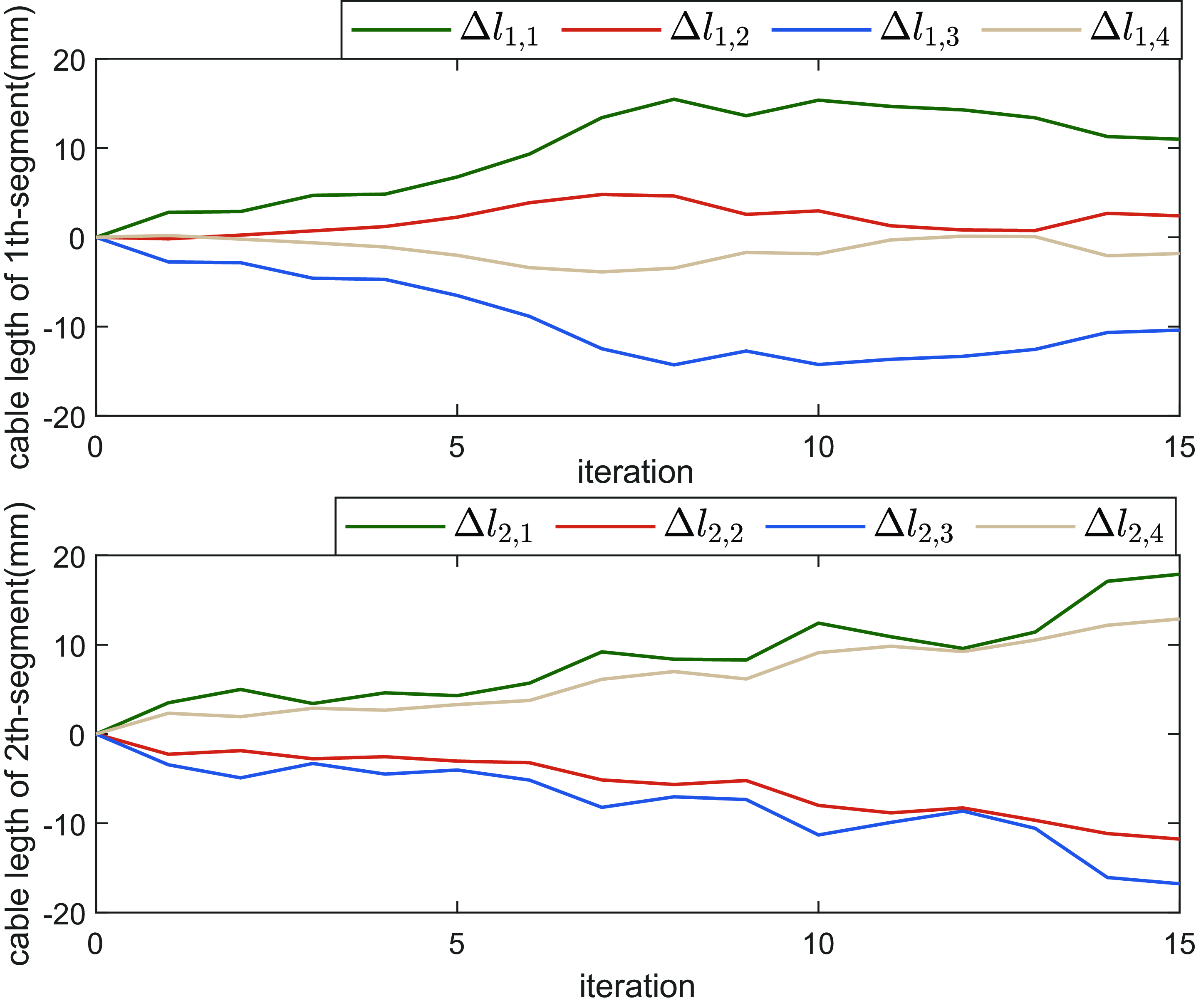
Figure 8. The length variation of the actuated cables for the obstacle avoidance planning.

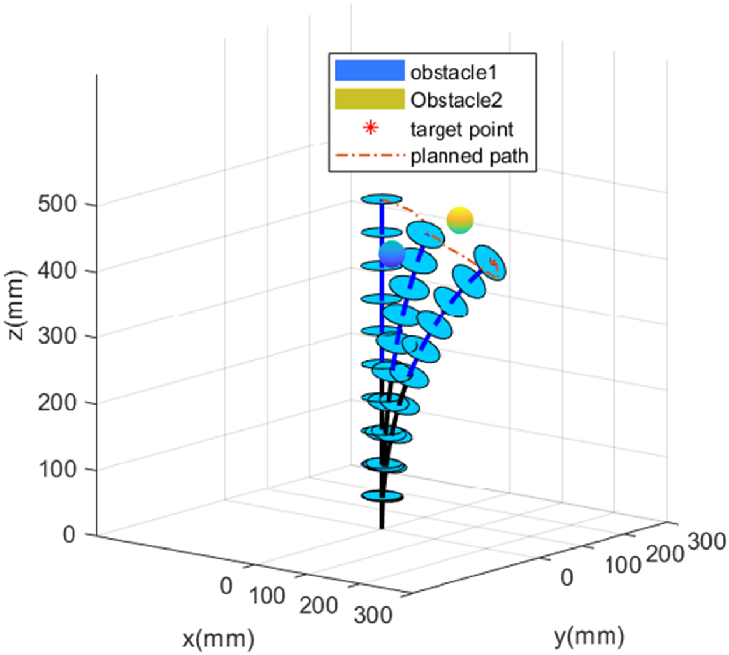
Figure 9. Path planning in the multi-obstacles environment.

The step size of $\lambda _t$ and $\delta _t$ should be chosen based on the task requirements of the system for that the step size should be taken large when the continuum robot is far from the target point to better improve the speed of path generation, and meanwhile, the small step size should be set to improve the planning accuracy when reaching near the target point. According to engineering experience, the decay function for step size can be designed as

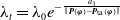(18) \begin{equation} {\lambda _t} ={\lambda _0}{e^{ - \frac{{{a_1}}}{{\left \|{{\boldsymbol{P}}\left ({\boldsymbol{\varphi }} \right ) -{{\boldsymbol{P}}_{\mathrm{ta}}}\left ({\boldsymbol{\varphi }} \right )} \right \|}}}} \end{equation}

(19) \begin{equation} {\delta _t} ={a_2}{\lambda _t} \end{equation}

where $\lambda _0$ , $a_1$ and $a_2$ are normal numbers.

Figure 10. Attitude angle curve for the obstacle avoidance planning.

Figure 11. The length variation of the actuated cables for the obstacle avoidance planning.

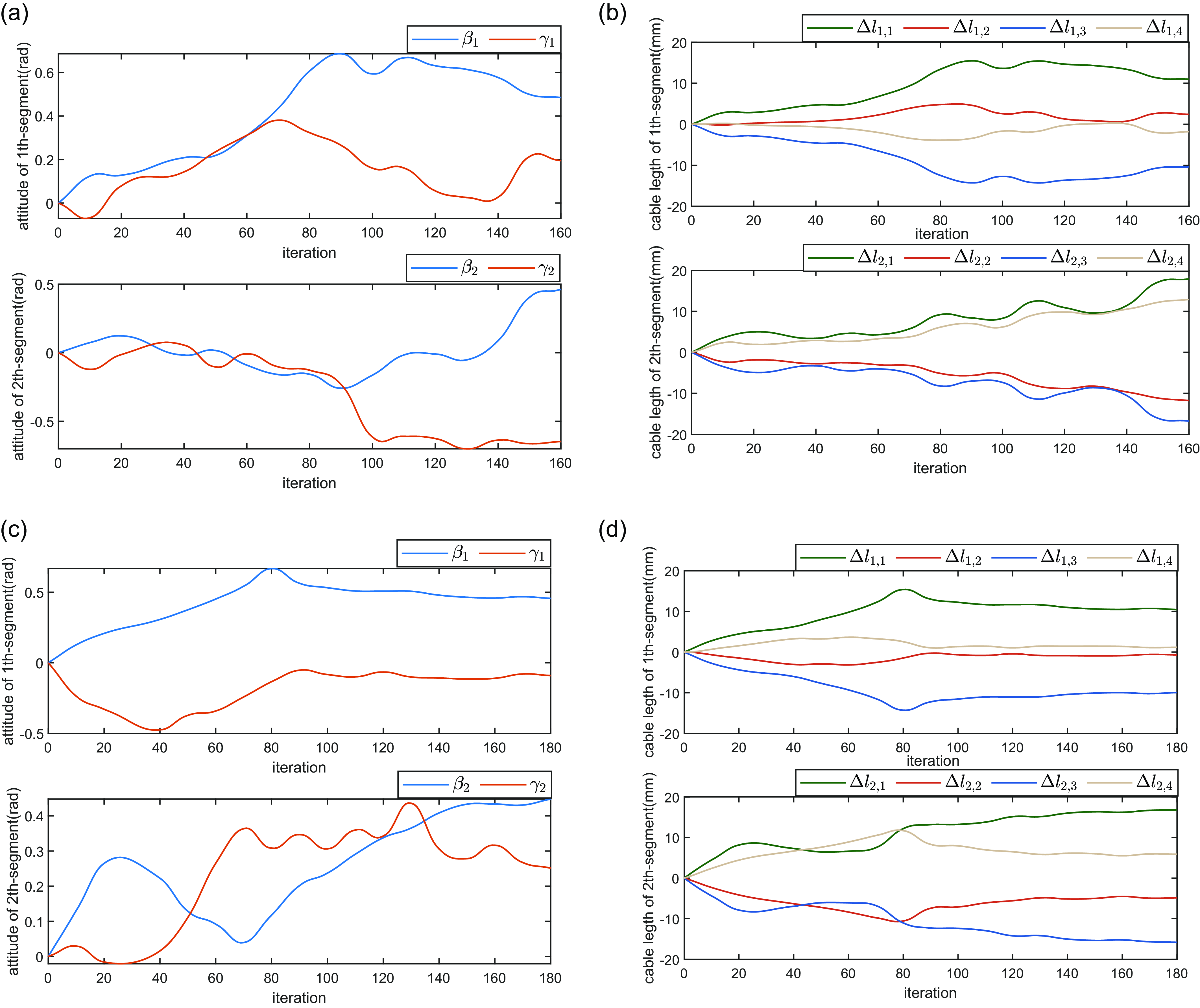
Figure 12. Curves of attitude angle and cable length after interpolation processing.

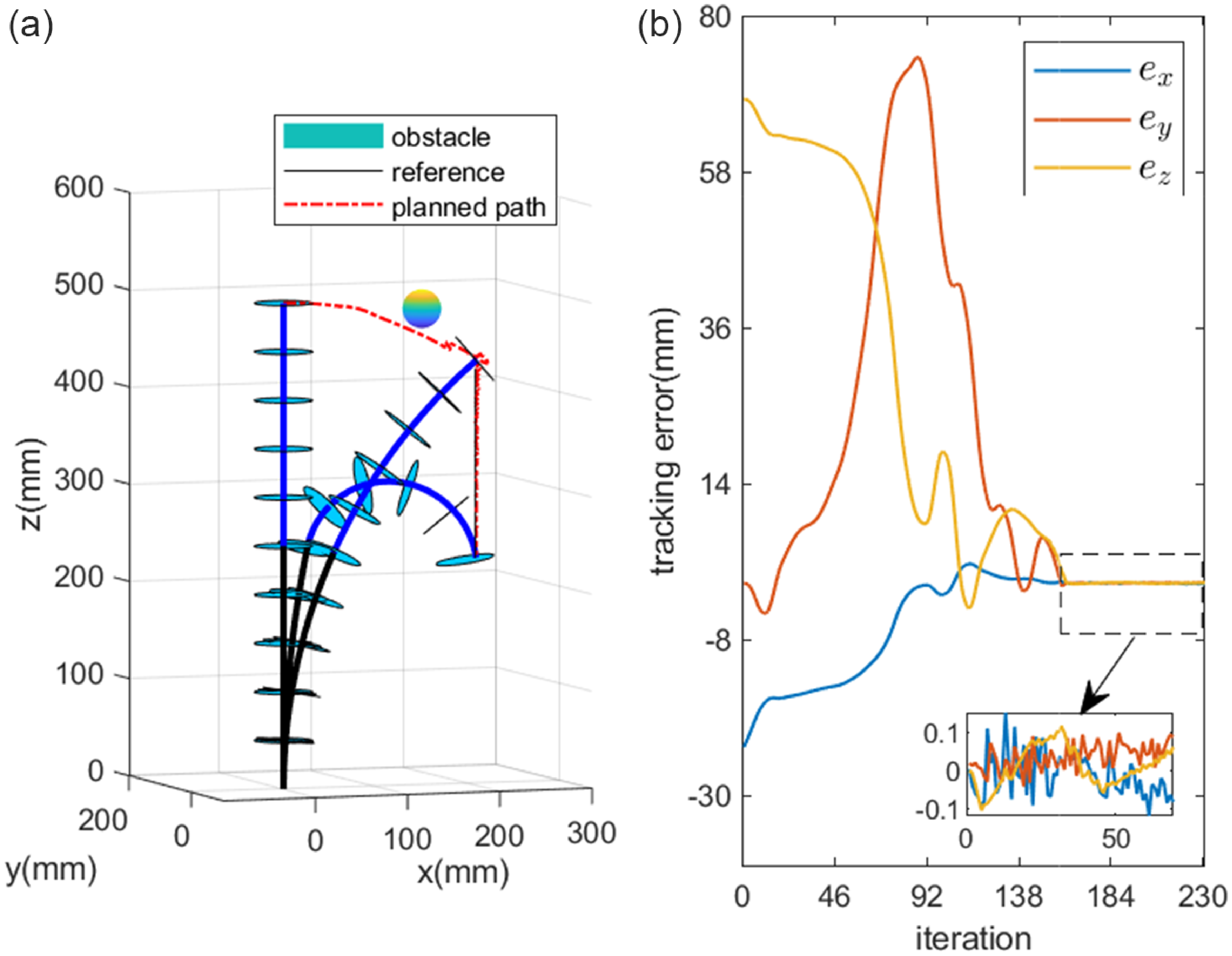
Figure 13. Trajectory tracking for two-segment continuum robot.

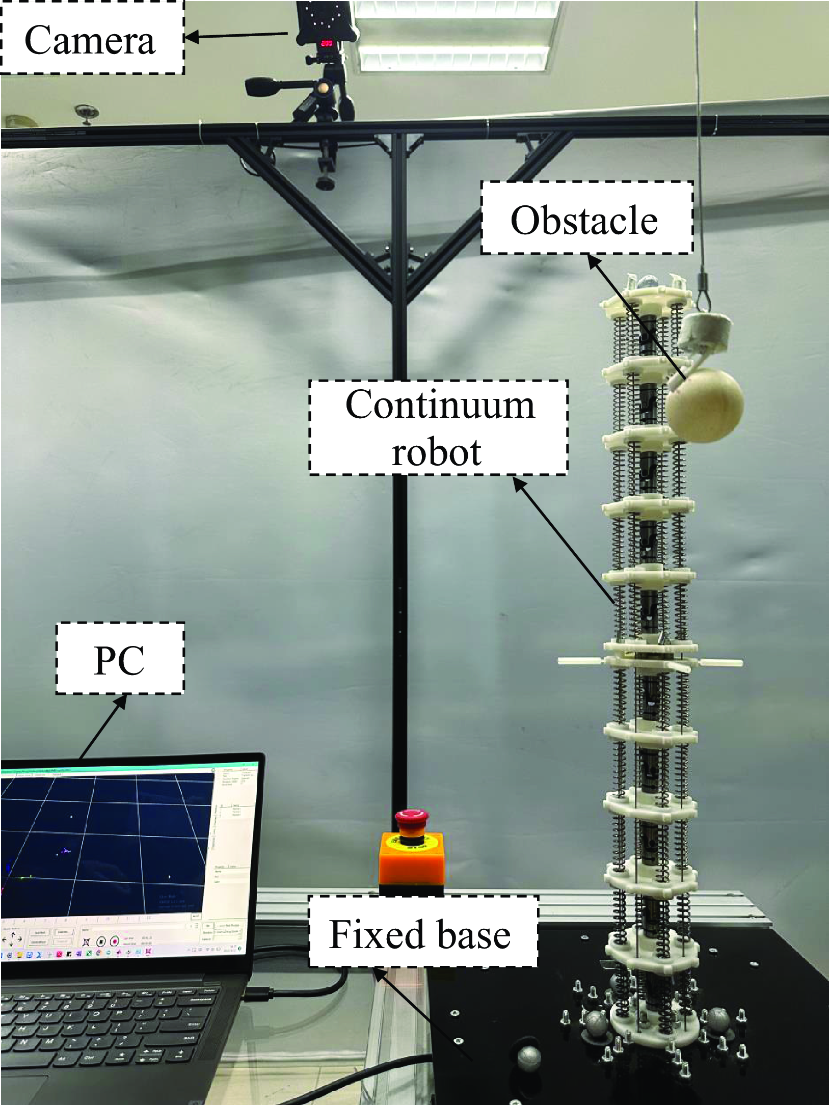
Figure 14. Two-segment cable-driven continuum robot prototype.

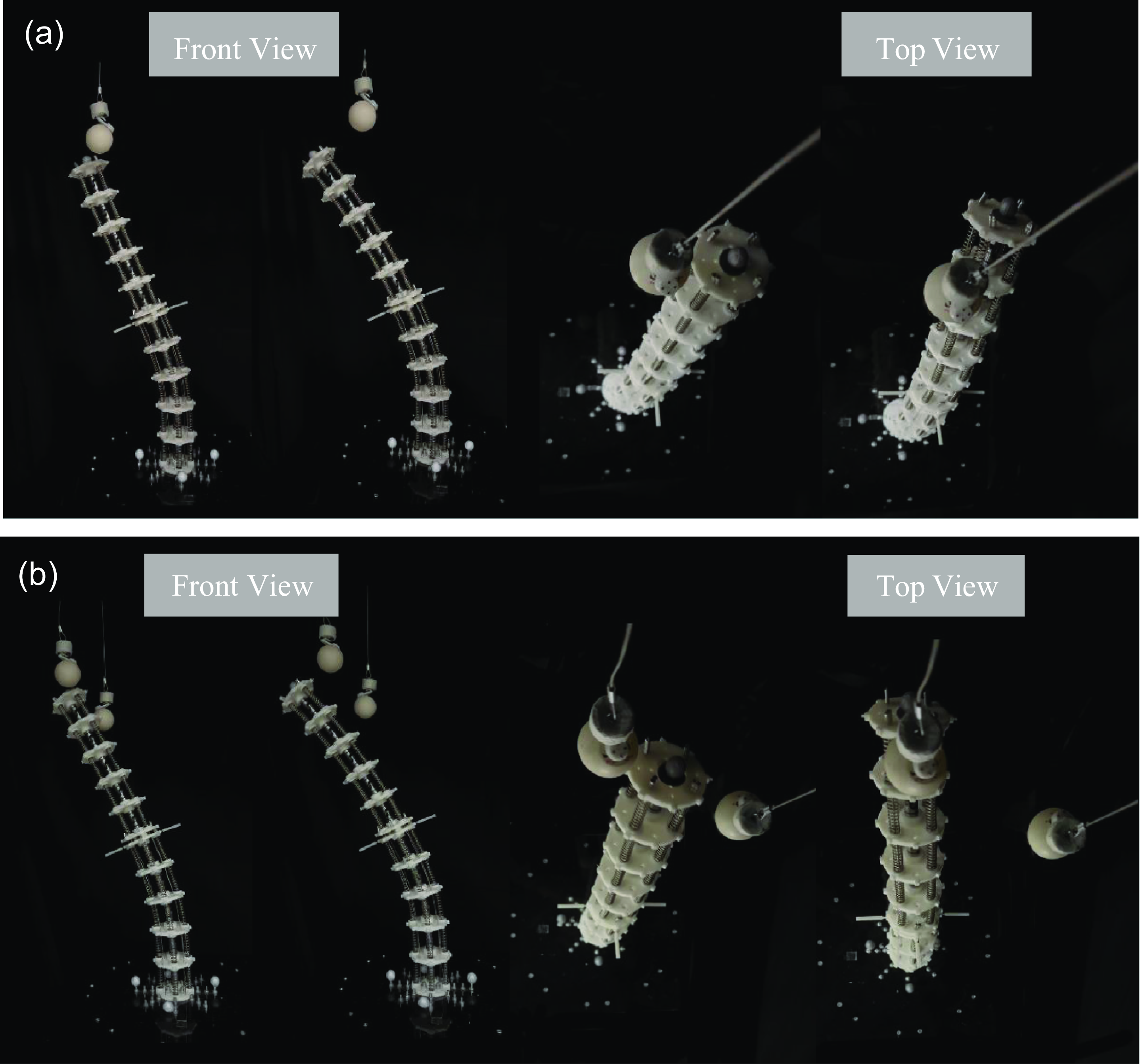
Figure 15. (a) Moving process in the single obstacle environment and (b) moving process in the multi-obstacles environment.

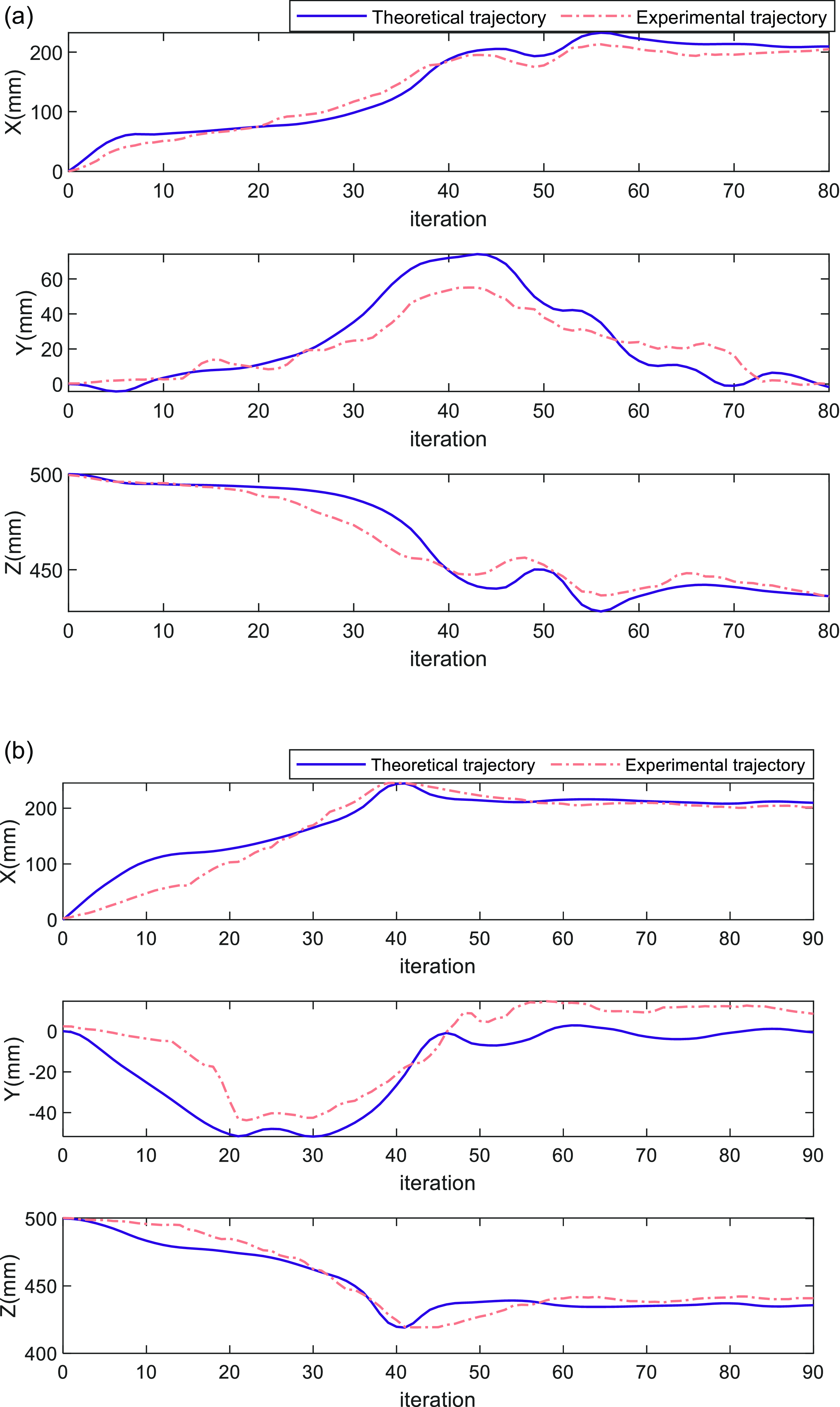
Figure 16. (a) Coordinate curves in the single obstacle environment and (b) coordinate curves in the multi-obstacles environment.

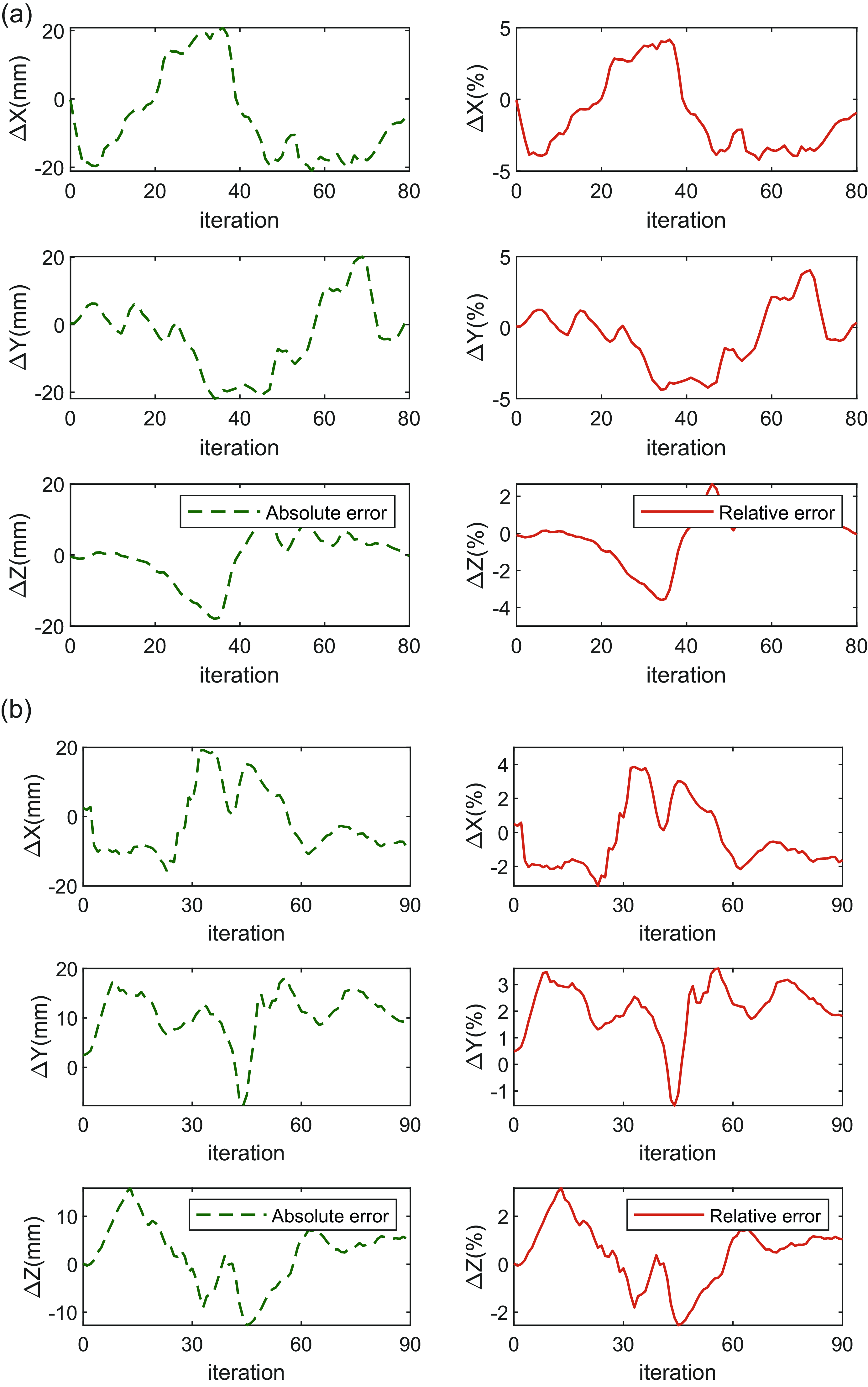
Figure 17. (a) Errors of planned path in the single obstacle environment and (b) errors of planned path in the multi-obstacles environment.

4.1. Simulation

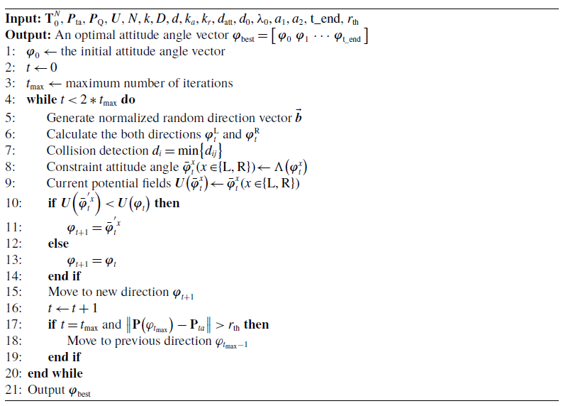
The proposed BAS-APF algorithm is firstly applied to path planning in the single obstacle environment. Assume that the initial attitude angle of the continuum robot is ${{\boldsymbol{\varphi }}_0} ={\left [{0,0,0,0} \right ]^{\mathrm{T}}}$ rad, the center of the obstacle is set as ${{\boldsymbol{P}}_{\mathrm{Q}}} = \left [{150,0,490} \right ]$ mm, the radius of the obstacle is 20 mm, the target point position is set as ${{\boldsymbol{P}}_{\mathrm{ta}}} = \left [{207.96,0,431.75} \right ]$ mm. The other parameters for the simulation are $d = 30$ mm, ${d_0} = 60$ mm, $k = 5$ , ${k_{\mathrm{a}}} = 10$ , ${k_{\mathrm{r}}} = 1$ , ${a_1} = 10$ , ${a_2} = 1$ , $r_{\mathrm{th}}$ .

Figure 6 shows the comparative performance of the motion path to avoid a single obstacle. It can be seen that although the APF method based on traversing approach can avoid the obstacle well and reach the target position for the continuum robot, it needs to perform more iterations for the planning task and the planned path is much longer than that with the proposed BAS-APF method. Figures 7 and 8 show the attitude angle and cable length of each segment under the proposed algorithm respectively.

For the path planning in the two obstacles environment, the centers of the obstacles are set as ${{\boldsymbol{P}}_{\mathrm{Q1}}} = \left [{150,0,490} \right ]$ mm and ${{\boldsymbol{P}}_{\mathrm{Q2}}} = \left [{100, - 100,450} \right ]$ mm, respectively. The values of other parameters are the same as the above simulation. The motion path of the continuum robot to avoid two obstacles is shown in Fig. 9. The corresponding planned attitude angle and cable length of each segment are shown in Figs. 10 and 11.

From the above simulations, we can see that the proposed BAS-APF method shows good performance for the path planning in single obstacle and multi-obstacles environments, especially in terms of the fast planning speed, which benefits from the design of searching variable step size. It is worth pointing out that the changes of attitude angle and cable length are discontinuous during iterations, which is not suitable for the actual system. However, this paper only discusses the path planning in the task space, while the planning method of configuration space can be combined to make the attitude angle smoother in the subsequent practical application. Here, we chose the quintic spline to interpolate attitude angles [Reference Tomasz, Mateusz and Fatina41], where the spline function is defined piecewise on each adjacent attitude angle interval and shown as:

(20) \begin{equation} {S_i}(\theta ) = a{}_i +{b_i}{\left ({\theta -{k_i}} \right )^2} +{c_i}{\left ({\theta -{k_i}} \right )^3} +{d_i}{\left ({\theta -{k_i}} \right )^4} +{e_i}{\left ({\theta -{k_i}} \right )^5} \end{equation}

where $\theta$ represents the attitude variable, $k_i$ is attitude note of the spline, $a{}_i,b{}_i,c{}_i,d{}_i$ and $e{}_i$ are constant coefficients. Thus, the curves of attitude angle and cable length after interpolation processing are shown in Fig. 12.

To evaluate the performance of the proposed algorithm regarding trajectory tracking, the continuum robot was tasked with tracking a straight-line trajectory utilizing the following parametric equation:

(21) \begin{equation} {{\textbf{x}}_r} ={{\textbf{P}}_{{\mathrm{ta}}}} +{\left [{\begin{array}{*{20}{c}} 0&0&{ - 2.85t} \end{array}} \right ]^{\mathrm{T}}} \end{equation}

where ${{\textbf{P}}_{{\mathrm{ta}}}} = \left [{207.96,0,431.75} \right ]$ is the initial point of the straight-line, $t \in \left [{0,70} \right ]$ donates the number of iterations.

Figure 13 (a) illustrates the motion of the robot end-effector along the straight-line trajectory. Initially, the continuum robot needs to move from its starting configuration to the starting position of the reference trajectory, while avoiding obstacles. Upon reaching the starting position, the robot tracks the reference trajectory precisely. Figure 13 (b) displays the tracking error of the end-effector after interpolation and the error remains within the range of [−0.2, 0.2] mm while moving along the straight-line trajectory.

4.2. Experimental verification

The experiment is designed to verify the obstacle avoidance planning effect of the continuum robot by adopting the proposed path planning method. Figure 14 shows the physical prototype platform of a two-segment cable-driven continuum robot. The two planned paths obtained from above simulation are executed by sending the cable length to the controller, and the moving process in two obstacle environments is shown in Fig. 15.

The continuum robot end moved along the desired path and avoided the obstacle well in both the cases. Figure 16 presents the experimental coordinate data of the continuum robot end in the base coordinate frame and Fig. 17 shows the error analysis between theoretical and experimental values. As shown in Fig. 17, the absolute error of each coordinate axis remains within the error band of $\left [{ - 20, + 20} \right ]$ mm and the relative error is controlled within 5 $\%$ . Compared to the ideal simulation, the continuum robot end in its initial vertical state has a certain offset from the base coordinate frame under the influence of gravity. Meanwhile, the prototype lacks a self-calibrating cable length mechanism where some of the actuated cables are slack in the initial motion, resulting in significant errors in the motion process. In addition, possible causes of errors include friction between ropes and holes, deformation of the elastic structures and measurement errors. Overall, the experimental results are in reasonable agreement with the simulation results.