


1. Introduction
Nowadays, accurate trajectories and dynamic responses of multibody systems play a key role in their performance. Moreover, mechanical systems are invading a broad range of applications, that is, medical, welding, and manufacturing robots. Thus, they became a crucial part of production systems. Consequently, ceaseless improvement and development of these systems to deliver more accurate responses emerge as an emergency. Nevertheless, the development is facing many challenges and limits deterring to meet the level of expectations mainly because of modeling limitations. In order to satisfy an already defined trajectory, designers proceed with path, motion, or function generation synthesis. Despite that mechanisms are not modeled as flexible in most synthesis approach, realistically this assumption results in errors between the real and predicted responses. Once a mechanism is manufactured, its prescribed trajectory and dynamics responses are different to the predicted ones using the synthesis approach. Therefore, compliant modeling should be deployed for the mechanism’s synthesis. Although synthesis analysis is limited to the mechanism end-effector trajectory, other responses should be considered for flexible mechanisms. Three different paradigms for formulating synthesis problems have been presented in the literature, mainly, path generation, motion generation, and function generation synthesis.
Rigid mechanisms synthesis based on path generation has been the scope of several works. Shaoping Bai et al. [Reference Bai and Angeles1] proposed a synthesis approach for a four-bar mechanism based on its coupler path. Sang Min Han et al. [Reference Han, In Kim and Kim2] have dealt with a topology optimization based on Fourier descriptors for path generation synthesis. The proposed approach has been tested through a set of illustrative examples. Yixin Shao et al. [Reference Shao, Xiang, Liu and Li3] have proposed a robotized gain rehabilitation system optimization, subsuming slider-crank and seven-bar mechanisms. The synthesis has been subject to dual-objective paths. The genetic algorithm (GA) has been deployed to optimize the system’s design parameters subject to constraints. A comparative analysis of the GA, the differential evolution (DE), and the imperialist competitive algorithm (ICA) for a rigid four-bar mechanism synthesis has been investigated in Saeed Ibrahimi et al. [Reference Ebrahimi and Payvandy4]. Volkan Parlaktaş et al. [Reference Parlaktaş, Söylemez and Tanik5] have optimized the design parameters for a geared four-bar mechanism subsuming collinear input and output shafts. Sahand Hadizadeh Kafash et al. [Reference Hadizadeh Kafash and Nahvi6] have treated a four-bar mechanism synthesis based on its generated path. By means of the circular proximity function, the error separating the obtained and target paths for each of its constitutive points has been evaluated. G. Ganesan et al. [Reference Ganesan and Sekar7] proposed a synthesis approach to overcome the filleted rectangular path generation challenges for an adjustable four-bar mechanism.
Another possible paradigm of the mechanisms synthesis relies on the motion generation. Jianwei Sun et al. [Reference Sun, Wang, Liu and Chu8] treated a planar four-bar mechanism synthesis based on the motion generation. Jean-François Collard et al. [Reference Collard, Duysinx and Fisette9] have dealt with extensible links mechanisms synthesis. The extensible links have been modeled by means of springs. Two optimization strategies have been deployed to solve the synthesis problem. The first minimizes each variable deviation during one cycle of the mechanism motion. Whereas the parameters have been simultaneously involved in the second strategy. The proposed approach efficiency has been investigated for two benchmark mechanisms synthesis, a four-bar, and a six-bar with extensible links. A multiphase motion generation synthesis for the four-bar mechanism has been the focus of Venkatesh Venkataramanujam et al. [Reference Venkataramanujam and Larochelle10].
In addition to path and motion generation synthesis, mechanisms synthesis can be carried out by means of function generation. A spatial spherical four-bar mechanism has been the interest of Rasim Alizade et al. [Reference Alizade and Gezgin11]. By means of six independent design variables, the Quaternion algebra has been deployed with the Chebychev approximation to provide optimal design variables. It has been proven that the Chebychev approximation error owns the best performance besides interpolation approximation, least square approximation, and fitting error extremums.
Although the major interest has been devoted to rigid mechanism, some works investigated compliant mechanism synthesis. Zhen Luo et al. [Reference Luo, Tong, Wang and Wang12] have treated a topology optimization for a compliant micro-inverter. To this end, a finite element approach, avoiding the Courant–Friedrichs–Lewy issues, has been developed. Three performance criteria have been considered for the topology optimization, mainly the geometrical advantage (GA), mechanical efficiency (ME), and mechanical advantage (MA). An enhanced synthesis approach combining both the dimensional and pose errors for a robot arm has been discussed in ref. [Reference Russo, Raimondi, Dong, Axinte and Kell13]. Numerical outcomes confirm the approach robustness to solve the synthesis problem for several scenarios.
Deepak et al. [Reference Deepak, Dinesh, Sahu and Ananthasuresh14] dealt with a compliant mechanism topology synthesis. A comparative analysis for a set of compliant mechanisms formulation, that is, inverter and gripper, has been presented. The mechanism’s efficiency, characteristic stiffness, and artificial spring formulations have been the key performance indicators for the numerical outcomes. A continuum 16-degree-of-freedom snake robot has been the interest of Abdelkhalick Mohammad et al. [Reference Mohammad, Russo, Fang, Dong, Axinte and Kell15]. An online algorithm has been developed allowing to follow the snake path and adjust it whenever needed. To this end, the coiled and uncoiled configurations of the robot have been considered. Another application of continuum robot has been treated in Anzhu work [Reference Gao, Li, Zhou, Wang and Liu16]. Different configurations for a contact-aided compliant mechanisms have been targeted in the numerical simulations. Experimental tests have been carried out to approve the numerical simulation outcomes. Chikhaoui et al. [Reference Chikhaoui, Granna, Starke and Burgner-Kahrs17] have focused on a design optimization of continuum robot. Both the design and control aspects of the dual-arm continuum robot have been optimized. Soft medical robot for cardiovascular application has been the scope of Liu Wang et al. [Reference Wang, Zheng, Harker, Patel, Guo and Zhao18]. The GA has been deployed to solve the design and optimization problem. Numerical outcomes corroborate well with the experimental data. The particle swarm optimization (PSO) has been deployed to find out optimal parameters subject to selected guides. Compliant mechanisms, taking into account their flexibility, have been treated in Nishiwaki et al. work [Reference Nishiwaki, Frecker, Min and Kikuchi19]. Based on the mutual energy concept, the flexible body has been modeled as linear elastic. Two cost function have been considered for multi-objective optimization problem. The first cost function has taken into account the kinematic aspect of the problem, whereas the second modeled the structural aspect. An illustrative example for a compliant gripper has been used to confirm the proposed approach efficiency.
Thanks to their outstanding performance to solve complex optimization problems, metaheuristics techniques have been deployed in complex mechanical systems optimization such as two fingers gripper [Reference Gholaminezhad and Jamali20], belt mechanism [Reference Lin and Hsiao21], unmanned vehicle [Reference Liu and Bucknall22], self-reconfigurable robot [Reference Zhang, Zhang and Gupta23], parallel manipulator [Reference Botello-Aceves, Valdez, Becerra and Hernandez24], delta parallel robot [Reference Brinker, Corves and Takeda25], biped robot [Reference Gupta and Dutta26], chamfered rectangle [Reference Ajith Kumar, Ganesan and Sekar27], multi-point haptic device [Reference Roberts and Rodriguez-Leal28], designing a bracket of a vehicle [Reference Yildiz and Erdaş29–Reference Panagant, Pholdee, Bureerat, Kaen, Yıldız and Sait32], robot gripper optimization [Reference Yildiz, Pholdee, Bureerat, Yildiz and Sait33], design of gear train [Reference Yildiz and Erdaş29], car crashworthiness [Reference Bureerat, Sait, Aye, Pholdee and Yildiz34–Reference Yıldız35], clutch diaphragm [Reference Yıldız, Pholdee, Panagant, Bureerat, Yildiz and Sait36], suspension arm [Reference Yildiz, Pholdee, Bureerat, Yildiz and Sait37–Reference Yıldız, Pholdee, Bureerat, Yıldız and Sait38], and parallelogram synthesis [Reference Valdez Peña, Chávez-Conde, Hernandez and Ceccarelli39]. All the references are compiled and classified based on the synthesis paradigm in Appendix Table AI.
In this work, the focus is concentrated on flexible mechanism synthesis. For the sake of more compliant modeling, the end-effector dynamic responses have been considered as target responses instead of its path. Moreover, the axial displacement of the flexible body has been involved in the synthesis problem to reduce emerging errors from considering such characteristic. Two benchmark flexible mechanisms, slider-crank and four-bar have been used for validation. The synthesis involves in first instance separately the slider velocity, and the axial displacement taking place in the flexible connecting rod. Subsequently, the previous responses, in addition to the slider acceleration, have been simultaneously combined into the same cost function. For the four-bar mechanism synthesis, five responses have been gathered, namely the crank, the flexible coupler, and the flexible follower midpoint paths in addition to the axial displacements of the flexible coupler and follower. A straightforward tool (Computer-Aided Design for Multibody systems Synthesis “CADMS”) has been created to perform the synthesis of the mechanism of interest using one or several optimization techniques among the GA, simulating annealing (SA), DE, PSO, ICA, Artificial Bee Colony (ABC), and the Ant Colony (AC). The main contributions of this work are as follows: (1) propose a synthesis approach for mechanisms synthesis considering the flexible parts, (2) consider both the dimensional and material characteristics as parameters in the synthesis approach, and (3) provide a straightforward executable tool “CADMS” under MATLAB software for flexible mechanism synthesis offering a wide range of selection among a set of metaheuristic techniques.
The paper is structured as follows: Section 2 deals with the dynamic modeling and the synthesis problem formulation of the two flexible mechanisms of scope. The different optimization algorithms used in this paper are discussed in Section 3. Section 4 denotes an insight into the proposed CADMS tool. Section 5 focuses on the main obtained results. The most important conclusions have been summarized in Section 6.
2. Mathematical formulation
To accomplish the objective of this work, an approach based on two modules is designed. The first is responsible on the dynamic modeling of flexible mechanism, whereas the second deals with the optimization process as depicted in Appendix Figure A2. They communicate together to ensure an exchange of data, that is, dynamic responses or optimal parameters.
2.1. Dynamics of a flexible mechanism
Dynamics modeling of flexible multibody systems has been of interest in tremendous works. Equation of motion are often a combination of algebraic equations defining the system’s holonomic constraints and differential equations. They involve the time derivative for the mechanism-independent parameters. Different approaches for solving differential-algebraic equations of flexible and rigid mechanisms have been discussed in refs. [Reference Shabana40–Reference Nikravesh44]. In this work, the dyad finite elements method has been used [Reference Romdhane, Dhuibi and Salah42] for the dynamic analysis of flexible slider-crank and four-bar mechanisms. It is suitable for flexible mechanism modeling with affordable computational burden. The flexible bodies of the mechanism are considered to be homogenous and isotropic. It is noteworthy that this study is limited only to purely linear elastic modeling of all flexible bodies with small deformation. Hence, all the assumptions of infinitesimal strain theory are fulfilled. Among the possible existing models in the literature for flexible beams, that is, Euler, Kirchhoff, and Cosset, the authors used Euler formulation with the dyad finite elements methods discussed in ref. [Reference Romdhane, Dhuibi and Salah42]. The ability to provide accurate results of the chosen method has been approved through experimental investigation presented in the aforementioned reference.

Figure 1. The general coordinates for a flexible beam.
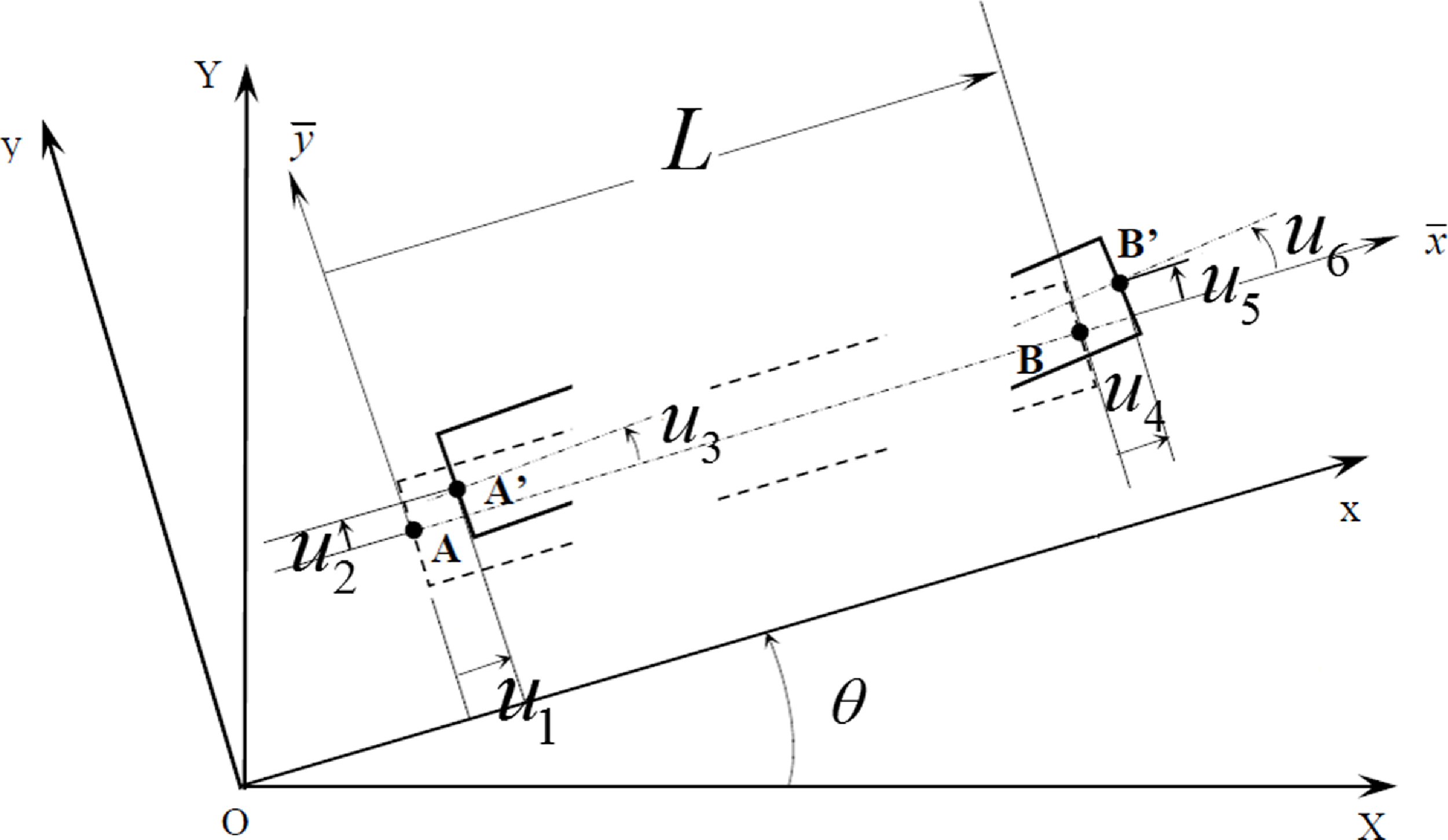
Figure 2. The flexible connecting rod in both rigid and deformed configurations.
The synthesis process is governed by an interaction between two parts. This process will be implemented in a graphical user interface tool discussed later in Section 4. While the optimization technique has been selected by the user (arrow 1), an initial random population is generated. Thereby, as depicted in Appendix Figure A2, a connection will be established with the dynamic model as pointed out by arrow number 2. Subsequently, the dynamic model will simulate their responses (arrow 3). In order to assess the accuracy of the dynamic responses, they are sent back to the optimization module (narrow 5). If the maximum iteration number is not yet reached, the algorithm will go back to arrow 1. Else, it will follow arrows 6 and 7 to stop the process. More details will be provided later in Section 4 for the implementation of this process into a graphical user interface. In what follows, the mathematical modeling for the Euler beam based on the Dyad finite elements [Reference Romdhane, Dhuibi and Salah42] is detailed.
The six general coordinates describing the flexible beam are detailed in Fig. 1. Mainly, two dyads constitute the flexible beam. Figure 2 depicts the six general coordinates $u_{1},u_{2},u_{3},u_{4},u_{5},u_{6}$
, for the flexible connecting rod. The absolute acceleration for a beam element can be written as shown in Eq. (1):
$u_{1},u_{2},u_{3},u_{4},u_{5},u_{6}$
, for the flexible connecting rod. The absolute acceleration for a beam element can be written as shown in Eq. (1):
 \begin{equation}\ddot{\boldsymbol{u}}_{\boldsymbol{a}}=\ddot{\boldsymbol{u}}_{\boldsymbol{r}}+\ddot{\boldsymbol{u}}+\boldsymbol{a}_{\boldsymbol{n}}+\boldsymbol{a}_{\boldsymbol{c}}+\boldsymbol{a}_{\boldsymbol{t}}\end{equation}
where $\ddot{\boldsymbol{u}}_{\boldsymbol{a}}$
is the absolute acceleration,
$\ddot{\boldsymbol{u}}_{\boldsymbol{a}}$
is the absolute acceleration, $\ddot{\boldsymbol{u}}_{\boldsymbol{r}}$
is the rigid element acceleration,
$\ddot{\boldsymbol{u}}_{\boldsymbol{r}}$
is the rigid element acceleration, $\ddot{\boldsymbol{u}}$
is the generalized relative acceleration,
$\ddot{\boldsymbol{u}}$
is the generalized relative acceleration, $\boldsymbol{a}_{\boldsymbol{n}}$
is the normal acceleration,
$\boldsymbol{a}_{\boldsymbol{n}}$
is the normal acceleration, $\boldsymbol{a}_{\boldsymbol{c}}$
is Coriolis, and
$\boldsymbol{a}_{\boldsymbol{c}}$
is Coriolis, and $\boldsymbol{a}_{\boldsymbol{t}}$
is tangential accelerations.
$\boldsymbol{a}_{\boldsymbol{t}}$
is tangential accelerations.
For this work, due to the small strain formulation assumption, only two components of the Eq. (1) are considered, the rigid element acceleration and the generalized relative acceleration. The new equation for the beam element acceleration yields
 \begin{equation}\ddot{u}_{a}=\ddot{u}_{r}+\ddot{u}\end{equation}
where $\ddot{\boldsymbol{u}}_{\boldsymbol{a}}$
is the absolute acceleration,
$\ddot{\boldsymbol{u}}_{\boldsymbol{a}}$
is the absolute acceleration, $\ddot{\boldsymbol{u}}_{\boldsymbol{r}}$
is the rigid element acceleration, and
$\ddot{\boldsymbol{u}}_{\boldsymbol{r}}$
is the rigid element acceleration, and $\ddot{\boldsymbol{u}}$
is the generalized relative acceleration.
$\ddot{\boldsymbol{u}}$
is the generalized relative acceleration.
Since the connecting rod is considered flexible, an axial displacement should take place along the x-axis and expressed as follows:
 \begin{equation}v(\bar{x},t)=\phi _{1}(\bar{x})u_{1}(t)+\phi _{4}(\bar{x})u_{4}(t)\end{equation}
where $u_{1}(t)$
and
$u_{1}(t)$
and $u_{4}(t)$
are the general coordinates detailed in Fig. 1.
$u_{4}(t)$
are the general coordinates detailed in Fig. 1. $\phi _{1}(\bar{x})$
and
$\phi _{1}(\bar{x})$
and $\phi _{4}(\bar{x})$
are the shape functions.
$\phi _{4}(\bar{x})$
are the shape functions.
The y-axis transversal displacement is written in Eq. (4) as:
 \begin{equation}w(\bar{x},t)=\phi _{2}(\bar{x})u_{2}(t)+\phi _{3}(\bar{x})u_{3}(t)+\phi _{5}(\bar{x})u_{5}(t)+\phi _{6}(\bar{x})u_{6}(t)\end{equation}
where $u_{2}(t)$
,
$u_{2}(t)$
, $u_{3}(t)$
,
$u_{3}(t)$
, $u_{5}(t)$
, and
$u_{5}(t)$
, and $u_{6}(t)$
are the general coordinates detailed in Fig. 1.
$u_{6}(t)$
are the general coordinates detailed in Fig. 1. $\phi _{2}(\bar{x})$
,
$\phi _{2}(\bar{x})$
, $\phi _{3}(\bar{x})$
,
$\phi _{3}(\bar{x})$
, $\phi _{5}(\bar{x})$
, and
$\phi _{5}(\bar{x})$
, and $\phi _{6}(\bar{x})$
are the shape functions.
$\phi _{6}(\bar{x})$
are the shape functions.
Several conditions should be fulfilled by the shape function used to model the flexible bodies of the mechanism. The shape functions should ensure the continuity within the element as well as in the boundaries related to other elements. In addition, the shape function should consider the stress and strain during the link deformation. Moreover, the boundaries compatibility for the displacement must be satisfied. To meet these requirements, the shape functions have been chosen as:
 \begin{align*} & \phi _{1}(\bar{\boldsymbol{x}})=1-\frac{\bar{\boldsymbol{x}}}{L} ;\, \phi _{4}(\bar{\boldsymbol{x}})=\frac{\bar{\boldsymbol{x}}}{L} ;\, \phi _{2}(\bar{x})=3\!\left(\frac{L-\bar{x}}{L}\right)^{2}-2\!\left(\frac{L-\bar{x}}{L}\right)^{3} ;\, \phi _{3}(\bar{x})=\bar{x}\!\left(\frac{L-\bar{x}}{L}\right)^{2} ;\\& \phi _{5}(\bar{x})=3\!\left(\frac{\bar{x}}{L}\right)^{2}-2\!\left(\frac{\bar{x}}{L}\right)^{3} ;\, \phi _{6}(\bar{x})=-L(L-\bar{x})\left(\frac{\bar{x}}{L}\right)^{2}\end{align*}
where $L$
is the total length of the flexible beam.
$L$
is the total length of the flexible beam.
The motion equation, based on the Lagrange principle for a flexible beam, yields
 \begin{equation}\frac{d}{dt}\left(\frac{\partial T}{\partial \dot{u}_{i}}\right)-\frac{\partial T}{\partial u_{i}}+\frac{\partial U}{\partial u_{i}}=\bar{Q}_{i}\end{equation}
where T, U and $Q_{i}$
are, respectively, the kinetic energy, the deformation energy, and the external forces applied to the beam element.
$Q_{i}$
are, respectively, the kinetic energy, the deformation energy, and the external forces applied to the beam element. $u_{i}$
and
$u_{i}$
and $\dot{u}_{i}$
are respectively the general coordinate and the velocity of the i
th
coordinate.
$\dot{u}_{i}$
are respectively the general coordinate and the velocity of the i
th
coordinate.
Consequently, the kinetic energy matrix form can be expressed as:
 \begin{equation}T=\frac{1}{2}\dot{\boldsymbol{u}}^{T}\bar{\boldsymbol{m}}\dot{\boldsymbol{u}}\end{equation}
where $\dot{\boldsymbol{u}}, \dot{\boldsymbol{u}}^{T}$
are the first derivative with respect of time for the local coordinates vector and its transpose, respectively.
$\dot{\boldsymbol{u}}, \dot{\boldsymbol{u}}^{T}$
are the first derivative with respect of time for the local coordinates vector and its transpose, respectively. $\bar{\boldsymbol{m}}$
is the elementary inertia matrix in the local coordinates of the beam.
$\bar{\boldsymbol{m}}$
is the elementary inertia matrix in the local coordinates of the beam.
The reduced matrix formulation for the deformation energy yields
 \begin{equation}U=\frac{1}{2}\boldsymbol{u}^{T}\bar{\boldsymbol{k}}\boldsymbol{u}\end{equation}
where $\boldsymbol{u}$
and
$\boldsymbol{u}$
and $\boldsymbol{u}^{T}$
are the general coordinates vector and its transpose.
$\boldsymbol{u}^{T}$
are the general coordinates vector and its transpose. $\bar{\boldsymbol{k}}$
is the elementary stiffness matrix in the local coordinates of the beam.
$\bar{\boldsymbol{k}}$
is the elementary stiffness matrix in the local coordinates of the beam.
Following [Reference Romdhane, Dhuibi and Salah42], a single dyad motion equation, in the flexible beam, regarding its local frame is written as:
 \begin{equation}\bar{\boldsymbol{m}}\ddot{\boldsymbol{u}}_{a}+\bar{\boldsymbol{k}}\boldsymbol{u}=\bar{\boldsymbol{Q}}\end{equation}
where $\bar{\boldsymbol{Q}}$
is the general forces vector expressed in the local frame.
$\bar{\boldsymbol{Q}}$
is the general forces vector expressed in the local frame.
The local and global coordinates are related by means of the following equation:
 \begin{equation}\boldsymbol{u}=\boldsymbol{RU}\end{equation}
The rotation matrix is expressed as shown in Eq. 10:
 \begin{equation} \mathbf{R}=\left[\begin{array}{c@{\quad}c@{\quad}c@{\quad}c@{\quad}c@{\quad}c} \lambda & \mu & 0 & 0 & 0 & 0\\[4pt] -\mu & \lambda & 0 & 0 & 0 & 0\\[4pt] 0 & 0 & 1 & 0 & 0 & 0\\[4pt] 0 & 0 & 0 & \lambda & \mu & 0\\[4pt] 0 & 0 & 0 & -\mu & \lambda & 0\\[4pt] 0 & 0 & 0 & 0 & 0 & 1 \end{array}\right] \end{equation}
where $\lambda =\cos \theta _{3}, \mu =\sin \theta _{3}$
and
$\lambda =\cos \theta _{3}, \mu =\sin \theta _{3}$
and $\boldsymbol{U}$
is the general coordinates vector expressed in the global frame.
$\boldsymbol{U}$
is the general coordinates vector expressed in the global frame.
The global kinetic energy regarding the global frame is written as shown in Eq. 11:
 \begin{equation}T=\frac{1}{2}\dot{\boldsymbol{U}}^{T}\boldsymbol{m}\dot{\boldsymbol{U}}\end{equation}
where
 \begin{equation}\boldsymbol{m}=\boldsymbol{R}^{\boldsymbol{T}}\bar{\boldsymbol{m}}\boldsymbol{R}\end{equation} $\boldsymbol{m}$
is the mass matrix in the global frame.
$\boldsymbol{m}$
is the mass matrix in the global frame.
In a similar way, the flexible beam deformation energy yields
 \begin{equation}V=\frac{1}{2}\boldsymbol{U}^{T}\boldsymbol{kU}\end{equation}
wherein
 \begin{equation}\boldsymbol{k}=\boldsymbol{R}^{\boldsymbol{T}}\bar{\boldsymbol{k}}\boldsymbol{R}\end{equation} $\boldsymbol{k}$
is the stiffness matrix in the global coordinates.
$\boldsymbol{k}$
is the stiffness matrix in the global coordinates.
Basically, two dyads constitute the flexible beam instilled in the mechanism. Hereby, both kinetic and deformation energies for the whole mechanism yield
 \begin{equation}T=\frac{1}{2}\left\{\dot{U}_{i}\right\}^{T}\boldsymbol{M}\!\left\{\dot{U}_{i}\right\}\end{equation}
where $\boldsymbol{M}$
is the assembling mass matrix.
$\boldsymbol{M}$
is the assembling mass matrix.
 \begin{equation}U=\frac{1}{2}\left\{U_{i}\right\}^{T}\boldsymbol{K}\!\left\{U_{i}\right\}\end{equation}
where $\boldsymbol{K}$
is the assembling stiffness matrix.
$\boldsymbol{K}$
is the assembling stiffness matrix.
The global motion equation relative to the flexible mechanism relying on the dyad finite element method, considering the beam structural damping, yields
 \begin{equation}M\ddot{U}+C\dot{U}+KU=-M\ddot{U}_{r}\end{equation}
where $\ddot{U}_{r}$
is the acceleration vector.
$\ddot{U}_{r}$
is the acceleration vector.
The damping matrix has been defined in ref. [Reference Sandor and Erdman45] as:
 \begin{equation}C_{k}=2\zeta _{k}\omega _{k}\theta _{t}\theta _{k}^{T}\end{equation}
where $\theta _{k}=M\phi _{k}$
,
$\theta _{k}=M\phi _{k}$
, $\zeta _{k}$
is the damping coefficient,
$\zeta _{k}$
is the damping coefficient, $\omega _{k}$
is the k
th eigenfrequency, and
$\omega _{k}$
is the k
th eigenfrequency, and $\phi _{k}$
is the k
th eigenmode.
$\phi _{k}$
is the k
th eigenmode.
Based on the selected eigenmodes numbers, n, the damping matrix yields
 \begin{equation}C=\sum\nolimits_{k=1}^{n}C_{k}\end{equation}
The following Eq. (20) allows to solve the free vibration systems as first step. Consequently, the eigenvalues for the system can be defined. The next step for the resolution will be to solve the motion equation for the whole system. It should be highlighted that resolution of the motion equation is impossible without the first step:
 \begin{equation}K\phi _{n}=\omega _{n}^{2}M\phi _{k}\end{equation}
where $\phi _{n}$
and
$\phi _{n}$
and $\omega _{n}$
are, respectively, the eigenmode and the eigenfrequency.
$\omega _{n}$
are, respectively, the eigenmode and the eigenfrequency.
To be able to decouple Eq. (17), modal coordinates should be used as written in Eq. (21):
 \begin{equation}U=\Phi \eta,\dot{U}=\Phi \dot{\eta },\ddot{U}=\Phi \ddot{\eta }\end{equation}
where $\Phi$
and
$\Phi$
and $\eta$
are, respectively, the modal matrix and amplitude.
$\eta$
are, respectively, the modal matrix and amplitude.
Finally, Eq. (17) yields
 \begin{equation}\Phi ^{T}M\Phi \ddot{\eta }+\Phi ^{T}C\Phi \dot{\eta }+\Phi ^{T}K\Phi \eta =-\Phi ^{T}M\ddot{U}_{r}\end{equation}
As detailed previously, the target responses to satisfy are defined following the designer convenience (arrow 6 Appendix Figure A2). Given responses for the two mechanisms of scope, the flexible slider-crank and four-bar have been considered as a case of study to investigate the proposed synthesis approach efficiency (Fig. 3).
The characteristic parameters for the target mechanism responses are detailed in Table I.
Table I. The inputs parameters.


Figure 3. The flexible mechanisms: (a) slider crank and (b) four-bar.
2.2. The synthesis problem formulation
As pointed out in Section 1, the main novelty of this paper is flexible mechanism synthesis based on a single or multiple dynamic responses, that is, velocity, acceleration of the end-effector, or axial displacement for a flexible body. The difference between the proposed approach, compared to classic ones, is that it does not rely on the end-effector path but the dynamic responses instead. Moreover, the flexible body’s axial displacement is involved in the synthesis analysis. Hereby, the cost function ought to evaluate different response types with different scales. The synthesis problem is extended from its most commonly treated case dealing with dimensions, to involve additional specifications such as material density and young modulus. Mechanism synthesis has been often formulated as an optimization problem. Thus, acting on a set of parameters, the error between the target and obtained responses is minimized. The cost function should fit and accommodate all the responses. To do so, the error in each time increment is divided by the module of the difference between the extremum obtained in the response curve as witnessed in Fig. 4. Consequently, the error will be dimensionless and scaled independently from the response types allowing to compile different responses as linear combination. Based on the same core cost function, the synthesis problem has been formulated for the two mechanisms of interest in this work.

Figure 4. The error evaluation.
2.2.1 The mathematical formulation of the flexible slider-crank mechanism synthesis
Six design variables have been selected for the mechanism synthesis combining both dimensional and characteristic parameters. The idea behind picking similar parameters is to optimize and control flexible bodies stiffness in order to satisfy a desired axial displacement threshold. The design variables are $l_{2}$
for the crank length and
$l_{2}$
for the crank length and $l_{3},\rho,E,h,a$
, respectively, the flexible connecting rod length’s, material density’s, Young modulus’s, high’s as well as width’s.
$l_{3},\rho,E,h,a$
, respectively, the flexible connecting rod length’s, material density’s, Young modulus’s, high’s as well as width’s.
The core objective function (Eq. 23) is formulated to be generic and could apply to any response type, whether velocity, acceleration, or axial displacement. It provides normalized and dimensionless values. Thereby, combining different response types as linear combination into the same cost function could be henceforth, possible:
 \begin{equation}\textit{fitness}=\textit{Minimize}(f(R(X)))=\textit{Minimize}\left(f\!\left(R\!\left(l_{2},l_{3},\rho,E,h,a\right) \right)\right)\end{equation}
where
 \begin{equation}f\!\left(R\!\left(l_{2},l_{3},\rho,E,h,a\right) \right)=\sqrt{\frac{1}{N}\sum\nolimits_{i=1}^{N}\left[\frac{R_{i}\left(l_{2},l_{3},\rho,E,h,a\right)-R_{i}^{*}(l_{2}^{*},l_{3}^{*},\rho ^{*},E^{*},h^{*},a^{*})}{Max(R_{i} (l_{2},l_{3},\rho,E,h,a))-Min(R_{i} (l_{2},l_{3},\rho,E,h,a))}\right]^{2}}\end{equation}
 \begin{align}& \textit{Subject}\ to\colon \nonumber\\[2pt]& l_{2}\ \mathit{\cos }\ \theta _{2}+l_{3}\ \mathit{\cos }\ \theta _{3}-x_{3}=0\nonumber\\[2pt]& l_{2}\ \mathit{sin }\ \theta _{2}+l_{3}\ \mathit{sin }\ \theta _{3}=0\nonumber\\[2pt]& L_{b2}\leq l_{2}\leq U_{b2}\nonumber\\[2pt]& L_{b3}\leq l_{3}\leq U_{b3}\nonumber\\[2pt]& l_{2}\lt l_{3}\nonumber\\[2pt]& L_{b4}\leq \rho \leq U_{b4}\nonumber\\[2pt]& L_{b5}\leq E\leq U_{b5}\nonumber\\[2pt]& L_{b6}\leq a\leq U_{b6}\nonumber\\& L_{b7}\leq h\leq U_{b7}\end{align}
where R is the considered response and $\boldsymbol{X}=\hspace{0pt}\hspace{0pt}\hspace{0pt}(l_{2},l_{3},\rho,E,h,a)$
representing the design variables. The parameter
$\boldsymbol{X}=\hspace{0pt}\hspace{0pt}\hspace{0pt}(l_{2},l_{3},\rho,E,h,a)$
representing the design variables. The parameter $R_{i}(l_{2},l_{3},\rho,E,h,a)$
represents the mechanism given response using the design variable vector
$R_{i}(l_{2},l_{3},\rho,E,h,a)$
represents the mechanism given response using the design variable vector $\boldsymbol{X}$
, whereas
$\boldsymbol{X}$
, whereas $R_{i}^{*}(l_{2}^{*},l_{3}^{*},\rho ^{*},E^{*},h^{*},a^{*})$
represents the target response defined by the user. The subscript i for both the generated and target responses is related to the number of prescribed points (N) equal to 121 for an average of one acquisition point each 0.004 s along 0.48 s. The simulation time is chosen to cover two crank’s revolution.
$R_{i}^{*}(l_{2}^{*},l_{3}^{*},\rho ^{*},E^{*},h^{*},a^{*})$
represents the target response defined by the user. The subscript i for both the generated and target responses is related to the number of prescribed points (N) equal to 121 for an average of one acquisition point each 0.004 s along 0.48 s. The simulation time is chosen to cover two crank’s revolution.
Substituting the letter R in the core function (Eq. 24) yields to equations Eq. (26), (27), and (28) dealing respectively with the acceleration error f(A( $l_{2},l_{3},\rho,E,h,a$
)), velocity error f(V(
$l_{2},l_{3},\rho,E,h,a$
)), velocity error f(V( $l_{2},l_{3},\rho,E,h,a$
)), and axial displacement error f(D(
$l_{2},l_{3},\rho,E,h,a$
)), and axial displacement error f(D( $l_{2},l_{3},\rho,E,h,a$
)). The slider velocity, acceleration, as well as the connecting rod midpoint axial displacement are strongly dependent on the set of following parameters (
$l_{2},l_{3},\rho,E,h,a$
)). The slider velocity, acceleration, as well as the connecting rod midpoint axial displacement are strongly dependent on the set of following parameters ( $l_{2},l_{3},\rho,E,h,a$
):
$l_{2},l_{3},\rho,E,h,a$
):
 \begin{equation}{f}({A}({l}_{2},{l}_{3},\rho,{E},{h},{a}) )=\sqrt{\frac{1}{{N}}\sum\nolimits_{{i}=1}^{{N}}\left[\frac{{A}_{{i}}({l}_{2},{l}_{3},\rho,{E},{h},{a})-{A}_{{i}}^{{*}}({l}_{2}^{{*}},{l}_{3}^{{*}},\rho ^{{*}},{E}^{{*}},{h}^{{*}},{a}^{{*}})}{{Max}({A}_{{i}} ({l}_{2},{l}_{3},\rho,{E},{h},{a}))-{Min}({A}_{{i}} ({l}_{2},{l}_{3},\rho,{E},{h},{a}))}\right]^{2}}\end{equation}
 \begin{equation}f(V(l_{2},l_{3},\rho,E,h,a) )=\sqrt{\frac{1}{N}\sum\nolimits _{i=1}^{N}\left[\frac{V_{i}(l_{2},l_{3},\rho,E,h,a)-V_{i}^{*}(l_{2}^{*},l_{3}^{*},\rho ^{*},E^{*},h^{*},a^{*})}{Max(V_{i} (l_{2},l_{3},\rho,E,h,a)-Min(V_{i} (l_{2},l_{3},\rho,E,h,a)}\right]^{2}}\end{equation}
 \begin{equation}f(D(l_{2},l_{3},\rho,E,h,a) )=\sqrt{\frac{1}{N}\sum\nolimits _{i=1}^{N}\left[\frac{D_{i}(l_{2},l_{3},\rho,E,h,a)-D_{i}^{*}(l_{2}^{*},l_{3}^{*},\rho ^{*},E^{*},h^{*},a^{*})}{Max(D_{i} (l_{2},l_{3},\rho,E,h,a)-Min(D_{i} (l_{2},l_{3},\rho,E,h,a)}\right]^{2}}\end{equation}
The velocity (Eq. 27)) and acceleration (Eq. (26)) considered in this work are relative to the end-effector component. However, in Eq. (28), the considered axial displacement $D_{i}$
is taking place at the connecting rod midpoint. The combined optimization compiles the three mechanism responses into the same cost function. A weight coefficient has been allocated to each response as recommended in ref. [Reference Khemili, Ben Abdallah and Aifaoui46]. The combined error is governed by Eq. (29) as follows:
$D_{i}$
is taking place at the connecting rod midpoint. The combined optimization compiles the three mechanism responses into the same cost function. A weight coefficient has been allocated to each response as recommended in ref. [Reference Khemili, Ben Abdallah and Aifaoui46]. The combined error is governed by Eq. (29) as follows:
 \begin{align}f(D,V,A) & =\alpha f\!\left(D\!\left(l_{2},l_{3},\rho,E,h,a\right) \right)+\beta f\!\left(V\!\left(l_{2},l_{3},\rho,E,h,a\right) \right)+\gamma f(A (l_{2},l_{3},\rho,E,h,a))\nonumber\\[10pt]& =\alpha \sqrt{\frac{1}{N}\sum _{i=1}^{N}\left[\frac{D_{i}(l_{2},l_{3},\rho,E,h,a)-D_{i}^{*}(l_{2}^{*},l_{3}^{*},\rho ^{*},E^{*},h^{*},a^{*})}{Max(D (l_{2},l_{3},\rho,E,h,a))-Min(D (l_{2},l_{3},\rho,E,h,a))}\right]^{2}}\nonumber\\[10pt]& +\beta \sqrt{\frac{1}{N}\sum _{i=1}^{N}\left[\frac{V_{i}(l_{2},l_{3},\rho,E,h,a)-V_{i}^{*}(l_{2}^{*},l_{3}^{*},\rho ^{*},E^{*},h^{*},a^{*})}{Max(V (l_{2},l_{3},\rho,E,h,a))-Min(V (l_{2},l_{3},\rho,E,h,a))}\right]^{2}}\nonumber\\[10pt]& +\gamma \sqrt{\frac{1}{N}\sum _{i=1}^{N}\left[\frac{A_{i}(l_{2},l_{3},\rho,E,h,a)-A_{i}^{*}(l_{2}^{*},l_{3}^{*},\rho ^{*},E^{*},h^{*},a^{*})}{Max(A (l_{2},l_{3},\rho,E,h,a))-Min(A (l_{2},l_{3},\rho,E,h,a))}\right]^{2}}\end{align}
where $\alpha =0.4,\beta =\gamma =0.3$
based on the parametric study carried out in ref. [Reference Khemili, Ben Abdallah and Aifaoui46].
$\alpha =0.4,\beta =\gamma =0.3$
based on the parametric study carried out in ref. [Reference Khemili, Ben Abdallah and Aifaoui46].
2.2.2 The mathematical formulation for the flexible four-bar mechanism synthesis
Since the four-bar mechanism subsumes two flexible links, its synthesis should be treated differently. Usually, for rigid four-bar mechanisms, the focus is devoted to the coupler path. However, when flexible parts are considered, this approach could not be accurate. Consequently, the crank, flexible coupler, as well as the flexible follower midpoint drawn paths, are considered. In addition, to keep the axial displacement during the synthesis process in acceptable thresholds, both axial displacements of the coupler and follower have been considered toward the mechanism synthesis. By means of the proposed core cost function in Eq. (24), combining all the five responses is possible providing a scalable and dimensionless error:
 \begin{align}& f\!\left(l_{1},l_{2},l_{3},l_{4}\right)=\nonumber\\[5pt]& \sqrt{\frac{1}{N}\sum\nolimits _{i=1}^{N}\left[\left(\frac{{x_{cr}}_{i}\left(l_{1},l_{2},l_{3},l_{4}\right)-{x_{cr}}_{i}^{*}\left(l_{1}^{*},l_{2}^{*},l_{3}^{*},l_{4}^{*}\right)}{Max\!\left({x_{cr}}_{i}\left(l_{1},l_{2},l_{3},l_{4}\right)\right)-Min\!\left({x_{cr}}_{i}\left(l_{1},l_{2},l_{3},l_{4}\right)\right)}\right)^{2}+\left(\frac{{y_{cr}}_{i}\left(l_{1},l_{2},l_{3},l_{4}\right)-{y_{cr}}_{i}^{*}\left(l_{1}^{*},l_{2}^{*},l_{3}^{*},l_{4}^{*}\right)}{Max\!\left({y_{cr}}_{i}\left(l_{1},l_{2},l_{3},l_{4}\right)\right)-Min\!\left({y_{cr}}_{i}\left(l_{1},l_{2},l_{3},l_{4}\right)\right)}\right)^{2}\right]}\nonumber\\[5pt]& +\sqrt{\frac{1}{N}\sum\nolimits _{i=1}^{N}\left[\left(\frac{{x_{co}}_{i}(l_{1},l_{2},l_{3},l_{4})-{x_{co}}_{i}^{*}(l_{1}^{*},l_{2}^{*},l_{3}^{*},l_{4}^{*})}{Max({x_{co}}_{i}(l_{1},l_{2},l_{3},l_{4}))-Min({x_{co}}_{i}(l_{1},l_{2},l_{3},l_{4}))}\right)^{2}+\left(\frac{{y_{co}}_{i}(l_{1},l_{2},l_{3},l_{4})-{y_{co}}_{i}^{*}(l_{1}^{*},l_{2}^{*},l_{3}^{*},l_{4}^{*})}{Max({y_{co}}_{i}(l_{1},l_{2},l_{3},l_{4}))-Min({y_{co}}_{i}(l_{1},l_{2},l_{3},l_{4}))}\right)^{2}\right]}\nonumber\\[5pt]& +\sqrt{\frac{1}{N}\sum\nolimits _{i=1}^{N}\left[\left(\frac{{x_{fo}}_{i}(l_{1},l_{2},l_{3},l_{4})-{x_{fo}}_{i}^{*}(l_{1}^{*},l_{2}^{*},l_{3}^{*},l_{4}^{*})}{Max({x_{fo}}_{i}(l_{1},l_{2},l_{3},l_{4}))-Min({x_{fo}}_{i}(l_{1},l_{2},l_{3},l_{4}))}\right)^{2}+\left(\frac{{y_{fo}}_{i}(l_{1},l_{2},l_{3},l_{4})-{y_{fo}}_{i}^{*}(l_{1}^{*},l_{2}^{*},l_{3}^{*},l_{4}^{*})}{Max({y_{fo}}_{i}(l_{1},l_{2},l_{3},l_{4}))-Min({y_{fo}}_{i}(l_{1},l_{2},l_{3},l_{4}))}\right)^{2}\right]}\nonumber\\[5pt]& +\sqrt{\frac{1}{N}\sum\nolimits _{i=1}^{N}\left[\frac{D_{coxi}(l_{1},l_{2},l_{3},l_{4})-D_{coxi}^{*}(l_{1}^{*},l_{2}^{*},l_{3}^{*},l_{4}^{*})}{Max(D_{coxi}(l_{1},l_{2},l_{3},l_{4}))-Min(D_{coxi}(l_{1},l_{2},l_{3},l_{4}))}\right]^{2}}\nonumber\\[5pt]& +\sqrt{\frac{1}{N}\sum\nolimits _{i=1}^{N}\left[\frac{D_{foxi}(l_{1},l_{2},l_{3},l_{4})-D_{foxi}^{*}(l_{1}^{*},l_{2}^{*},l_{3}^{*},l_{4}^{*})}{Max(D_{foxi}(l_{1},l_{2},l_{3},l_{4}))-Min(D_{foxi}(l_{1},l_{2},l_{3},l_{4}))}\right]^{2}}\end{align}
 \begin{align}& \textit{Subject}\ to\colon \nonumber\\& l_{2}+l_{4}\lt l_{1}+l_{3}\nonumber\\& l_{2}+l_{3}\lt l_{1}+l_{4}\nonumber\\& l_{1}+l_{2}\lt l_{3}+l_{4}\nonumber\\ & L_{b1}\leq l_{1}\leq U_{b1}\nonumber\\& L_{b2}\leq l_{2}\leq U_{b2}\nonumber\\& L_{b3}\leq l_{3}\leq U_{b3} \nonumber\\& L_{b4}\leq l_{4}\leq U_{b4}\end{align}
Errors following the X and Y axis for the prescribed paths of the crank, coupler, and follower beside the target ones as well as axial displacements for the coupler and follower have been assessed. Errors have been measured among 121 points of the drawn responses. The cost function is formulated Eq. (30), where $l_{1},l_{2},l_{3},l_{4}$
and
$l_{1},l_{2},l_{3},l_{4}$
and $l_{1}^{*},l_{2}^{*},l_{3}^{*},l_{4}^{*}$
are respectively the generated and the reference design variables, where
$l_{1}^{*},l_{2}^{*},l_{3}^{*},l_{4}^{*}$
are respectively the generated and the reference design variables, where $l_{1}$
is the frame length,
$l_{1}$
is the frame length, $l_{2}$
is the crank length,
$l_{2}$
is the crank length, $l_{3}$
is the flexible coupler length, and
$l_{3}$
is the flexible coupler length, and $l_{4}$
is the flexible follower length. The parameters
$l_{4}$
is the flexible follower length. The parameters $x_{foi}{y_{fo}}_{i}x_{coi}{y_{co}}_{i}x_{cri}{y_{cr}}_{i}$
represent the coordinates along x and y axis for the follower, coupler, and crank midpoints, respectively. All variables labeled with the subscript (*) such as
$x_{foi}{y_{fo}}_{i}x_{coi}{y_{co}}_{i}x_{cri}{y_{cr}}_{i}$
represent the coordinates along x and y axis for the follower, coupler, and crank midpoints, respectively. All variables labeled with the subscript (*) such as ${{x^{*}}_{fo}}_{i}$
,
${{x^{*}}_{fo}}_{i}$
, ${{y^{*}}_{fo}}_{i}$
,
${{y^{*}}_{fo}}_{i}$
, ${{x_{co}}_{i}}^{*}$
,
${{x_{co}}_{i}}^{*}$
, ${{y_{co}}_{i}}^{*}$
,
${{y_{co}}_{i}}^{*}$
, $x_{cri}^{*}$
, and
$x_{cri}^{*}$
, and $y_{cri}^{*}$
characterize the target response coordinates, respectively, for the follower, coupler, and crank. D
cox
and D
fox
are respectively the coupler and follower axial displacements; meanwhile, D
*
cox
and D
*
fox
are the ones relative to the target response. L
b
and U
b
represent the lower and upper bounds for the search intervals of the design variables, respectively.
$y_{cri}^{*}$
characterize the target response coordinates, respectively, for the follower, coupler, and crank. D
cox
and D
fox
are respectively the coupler and follower axial displacements; meanwhile, D
*
cox
and D
*
fox
are the ones relative to the target response. L
b
and U
b
represent the lower and upper bounds for the search intervals of the design variables, respectively.
3. Resolution algorithms
Metaheuristics optimization techniques seem the most prominent to solve similar synthesis problems owing to their complexity. Therefore, several optimization techniques have been deployed in this work, that is, the GA [Reference Golderberg47], SA [Reference Kirkpatrick, Gelatt and Vecchi48], DE [Reference Storn and Price49], PSO [Reference Clerc50], Imperialist Colony Algorithm [Reference Atashpaz-Gargari and Lucas51], Artificial Bee Colony [Reference Karaboga and Basturk52], and the Ant Colony [Reference El-Hawary53]. The different algorithms pseudo-codes and how they have been adopted to the actual synthesis problem have been discussed detailed in ref. [Reference Ben Abdallah, Khemili and Aifaoui54]. Search intervals for the different parameters of the flexible slider-crank mechanism, namely, the crank length (l 1 ), the flexible connecting rod length (l 2 ), material density (ρ), Young Modulus (E) as well as the connecting rod high (h) and width (a), are summarized in Table II. L b , U b represent the lower and upper bounds for the search intervals of the design variables, respectively.
Table II. The different parameter search intervals for the slider-crank mechanism.

Four parameters have been of scope for the flexible four-bar mechanism, namely the frame length (l 1 ), the crank length (l 2 ), the coupler length (l 3 ), and the follower length (l 4 ). The different parameters search intervals have been summarized in Table III.
Table III. The different parameter search intervals for the four-bar mechanism.

4. Computer-Aided Design for Multibody systems Synthesis
The graphical interface is created to provide the user with a straightforward tool subsuming all necessary commands. The welcoming window gives the user the possibility to select the mechanism of interest as illustrated in Figure 5. The second window contains the run button, in addition to four main sections as shown in Figure 6 (response type synthesis, design variables, optimization techniques, and target responses). The slider acceleration or velocity, the connecting rod axial displacement, and the combined synthesis constitute the cornerstone of the slider-crank mechanism menu. On the other hand, the crank, the flexible follower, and the flexible coupler paths or a combination of all of them constitute the synthesis menu for the flexible four-bar mechanism.

Figure 5. The Computer-Aided Design for Multibody Synthesis (CADMS) graphical interface.

Figure 6. The flexible slider-crank mechanism synthesis menu.
Six design variables are of scope for the flexible slider-crank mechanism, mainly the crank (l2), the flexible connecting rod (l3) lengths, flexible connecting rod material density (ρ), and Young Modulus (E) as well as the connecting rod height (h) and width (a) as exhibited in Fig. 5. However, regarding the four-bar, the frame (l1), crank (l2), flexible coupler (l3), and flexible follower (l4) lengths are optimized (Fig. 7).
Possible search intervals avoiding any constraint violation are the constituents of the design variables menu. The tool can automatically evaluate any possible incoherence of the selected search intervals. If so, an error message will be displayed to help the user adjusting them. The choice of the optimization technique is possible through the third part of this tool titled optimization techniques. The last step before running the simulation is to introduce the target responses. Depending on the selected or available response data, the auspicious fitness function, expressed in Eqs. (26), (27), (28), (29), and (30), will be selected.
Finally, thanks to the run button the user can start the synthesis process. Subsequently, a post processing window pops up allowing to pick the desired response to plot as shown in Fig. 8. The illustrated case in Fig. 8, is for a combined synthesis selecting all the optimization techniques.

Figure 7. The four-bar mechanism synthesis menu.

Figure 8. The postprocessing window for the flexible slider-crank mechanism.
The next section compiles numerical outcomes for the proposed synthesis approach implemented in the Computer-Aided Design for Multibody systems Synthesis (CADMS) tool.
5. Results and discussions
Towards this section, the proposed approach for flexible mechanisms synthesis based on dynamic responses or axial displacement of a flexible part is investigated. Two responses, mainly the slider velocity and flexible connecting rod midpoint axial displacement, have been involved separately for the flexible slider-crank mechanism synthesis (Eqs. (27), (28)). Subsequently, the previous responses, in addition to the slider acceleration (Eq. (26)), have been involved in a combined synthesis (Eq. (29)). Five responses are of interest for the flexible four-bar mechanism, namely the crank, the coupler, and the follower midpoint paths’ as well as the coupler and follower axial displacements. The difference between the chosen responses for both mechanisms is strictly due to their industrial applications. Usually, for the slider-crank mechanism, the designer is interested in the end-effector dynamic responses. However, four-bar mechanisms are commonly used in complicated devices to satisfy a given path. It is noteworthy that considering the different component flexibility in the four-bar mechanism, the resulting path is pulled away from the target one. The obtained optimal solutions have been chosen based on statistical analysis for the obtained results over 100 runs of all the optimization techniques. A fitting for the outcome histograms has been made to approximate the distribution law and the key statistical metrics governing these results. The numerical simulations have been performed using an Intel I7 9th generation CPU computer.
5.1. Flexible slider-crank mechanism synthesis
5.1.1 Synthesis based on the slider velocity
As a first investigation for the proposed synthesis approach, the slider velocity has been chosen as a target response among the synthesis process. Statistical metrics confirm that the synthesis results corroborate well with a normal law distribution, wherein the mean $\mu$
and the standard deviation
$\mu$
and the standard deviation ${\sigma}$
are detailed in Appendix Table AII. The authors opted for the solution having the highest probability and the same or nearest mean
${\sigma}$
are detailed in Appendix Table AII. The authors opted for the solution having the highest probability and the same or nearest mean $\mu$
of the normal law distribution fitting as depicted in Appendix Figure A1. The deployed optimization techniques’ performances are compared according to this selection standard. It could be inferred that the Ant Colony (AC) technique outperforms the other ones proposing a set of design variables settling at a nil error. The DE method is less accurate with an error estimated of 1.8503 10-17. Accordingly, this is reflected in results of Figs. 9 and 10, respectively, for the slider velocity and acceleration through an overlapping for target and optimal responses. Nevertheless, a proportional discrepancy to the errors in Appendix Table AII is witnessed for the other optimization techniques. Although its low accuracy, the GA presents an interesting CPU time to conclude the required number of iterations. The results in Fig. 11 reveal difficulty to satisfy the axial displacement threshold based on the velocity synthesis. In perfect agreement with Kim’s work [Reference Kim, Seo and Kim55] for the first- and second-order derivative curves for mechanisms synthesis, satisfying the mechanism velocity results consequently in satisfying its acceleration.
$\mu$
of the normal law distribution fitting as depicted in Appendix Figure A1. The deployed optimization techniques’ performances are compared according to this selection standard. It could be inferred that the Ant Colony (AC) technique outperforms the other ones proposing a set of design variables settling at a nil error. The DE method is less accurate with an error estimated of 1.8503 10-17. Accordingly, this is reflected in results of Figs. 9 and 10, respectively, for the slider velocity and acceleration through an overlapping for target and optimal responses. Nevertheless, a proportional discrepancy to the errors in Appendix Table AII is witnessed for the other optimization techniques. Although its low accuracy, the GA presents an interesting CPU time to conclude the required number of iterations. The results in Fig. 11 reveal difficulty to satisfy the axial displacement threshold based on the velocity synthesis. In perfect agreement with Kim’s work [Reference Kim, Seo and Kim55] for the first- and second-order derivative curves for mechanisms synthesis, satisfying the mechanism velocity results consequently in satisfying its acceleration.

Figure 9. The slider velocity based on the slider velocity synthesis.
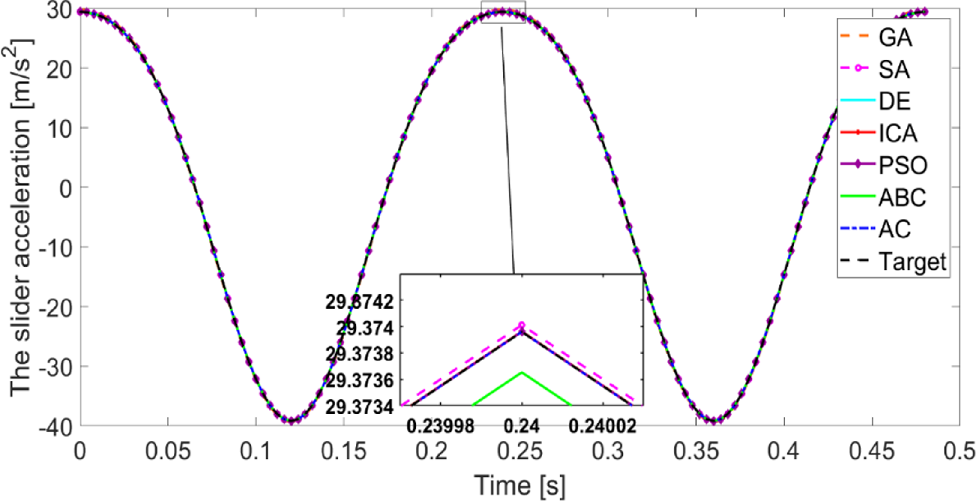
Figure 10. The slider acceleration based on the slider velocity synthesis.

Figure 11. The axial displacement based on the slider velocity synthesis.

Figure 12. The error evolution based on the slider velocity synthesis.
It can be witnessed in Fig. 12 that the error evolution as function of iteration number contains some flat area. Within these areas, the error remains constant. Optimization algorithms have a set of steps allowing them to test different random combination of parameters from the search interval. If the algorithm could not manage to retrieve a better solution, it will keep the one from the previous iteration. Hence, this justifies the constant error for some iterations.

Figure 13. Graphical summary for the performance of the optimization techniques based on the slider velocity, (a) for the slider velocity, (b) for the slider acceleration, and (c) for the axial displacement.
To emphasize the gap between the target and optimal responses retrieved by the optimization algorithms, a zoom focusing on specific area has been made as per Figs. 9 and 10. The responses of scope in this work are obtained by means of numerical integration of the motion equations. The minimum time step chosen in this work is 0.004 s. Consequently, any two successive points, separated by the time step, are linked with a straight line. For clarity purposes, it is useful to zoom beyond the time step interval. Therefore, linear areas can be visible in the zoom area.
It can be witnessed in Fig. 12 that the error evolution as function of the iteration number differs from one technique to another. As each of the used techniques is based on different algorithm, it should be expected that their performances will be different. This is in perfect agreement with previous works where different techniques have been used in optimization problems [Reference Ebrahimi and Payvandy4, Reference Zhang, Ning, Li, Pan, Gao and Zhang56–Reference Rout and Mittal60]. The GA common process consists of randomly generating initial population from the search intervals, selection, crossover, and mutation. This same process is governing the DE where the mutation is taking place before the crossover. For the SA technique, the process starts with generating the initial population to create subsequently new solution based on the mutation and evaluation steps. The mutation process in this case helps the algorithm to assess each solution with its neighbourhood in order to retrieve the best one. This will result consequently in building new population and updating the ever-best solution. The ant colony, particle swarm, and artificial bee colony are swarm-based algorithms. They are based on the swarm collaboration in their search for food. By analogy, the best food site is considered as optimal solution for the optimization problem. The search is based on the swarm communication and collaboration to find the best food site. Therefore, the algorithms manage to find the optimal solution. As the communication differs from birds to bees or ants, the optimal solution differs from one technique to another explaining the different levels of error in Fig. 12.
Fig. 13 depicts the performance of the optimization techniques. Ideally, the heptagon should be tangent to the green circle where the performance of the optimization technique is considered excellent. However as in Table IV, some of the techniques performances are limited or moderated, and the heptagon is tangent to either the red or amber circles for some techniques. Fig. 13 is a visual illustration of Table IV. An in-depth analysis for the results obtained in Appendix Table AII reveals that some of techniques can be more advantageous compared to others for the mechanism synthesis based on the slider velocity. Two main criteria are considered to assess the advantages and downsides of these techniques, mainly the calculation time to achieve the required number of iterations and the accuracy. The AC settle at a zero error for a CPU time of 3248 s. The DE manages to provide accurate results as well. However, the CPU time required is around 97% higher than the AC. It is worth considering the results of the GA as it requires as little as 30% of the CPU time for the AC. The low CPU time is the major advantage of the GA, making it very prominent for preliminary design stage synthesis.
Table IV. Summary of the synthesis results based on the velocity synthesis.

To make the results more understandable and readable, the performance of each optimization technique, based on the responses involved in the synthesis process, is summarized in Table IV. The performance of the optimization techniques has been assessed with, limited, moderated, or excellent based on how accurate the responses of the mechanism. In the next section, the mechanism synthesis is performed based on the axial displacement taking place in the connecting rod midpoint.
5.1.2 The axial displacement synthesis
This section is devoted to the synthesis results based on axial displacement threshold for the flexible connecting rod midpoint. It can be witnessed in Fig. 14 that this synthesis-based response is a burdensome task to accomplish. The errors evolution plotted in Fig. 14 have the mean $\mu$
parameter value of the normal distribution shown in Appendix Figure A3 and Appendix Table AIII. Figure 15 for the slider velocity depicts a considerable discrepancy beside the one taking place for the slider velocity synthesis. As witnessed in Fig. 16, the AC solution responses almost overlap the target ones. It is interesting to highlight that the ABC technique exhibits a good performance, as illustrated in Fig. 17, wherein error worth 1.25 103 despite a CPU time of 12,723 s.
$\mu$
parameter value of the normal distribution shown in Appendix Figure A3 and Appendix Table AIII. Figure 15 for the slider velocity depicts a considerable discrepancy beside the one taking place for the slider velocity synthesis. As witnessed in Fig. 16, the AC solution responses almost overlap the target ones. It is interesting to highlight that the ABC technique exhibits a good performance, as illustrated in Fig. 17, wherein error worth 1.25 103 despite a CPU time of 12,723 s.

Figure 14. The error evolution based on the flexible connecting rod midpoint axial displacement.

Figure 15. The slider velocity based on the axial displacement synthesis.

Figure 16. The slider acceleration based on the axial displacement synthesis.

Figure 17. The axial displacement based on the axial displacement synthesis.
The proposed design variables fulfil only the axial displacement illustrated in Fig. 17. These results corroborate well with the slider velocity synthesis results discussed in Section 5.1.1 proving that except for the involved response the other ones are dismissed. The performance of the different optimization techniques based on the axial displacement synthesis is assessed in Table V. Fig. 18 summarizes the results presented in Table V. The comparison of the different optimization techniques reveals that four out of the seven implemented techniques in this work have moderated performance. This is clearly seen through tangency of the heptagon to the amber circle for both the slider’s velocity and acceleration. The three other techniques have limited performances for the slider’s velocity and acceleration. For the axial displacement, the figure depicts almost a perfect heptagon included inside the moderated performance circle except from the GA edge where it is tangent to the red circle indicating a limited performance.
Table V. Summary of the synthesis results based on the axial displacement synthesis.
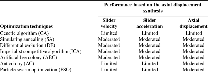

Figure 18. Graphical summary for the performance of the optimization techniques based on the axial displacement, (a) for the slider velocity, (b) for the slider acceleration, and (c) for the axial displacement.
5.1.3 The combined error synthesis
Based on the outcomes of Sections 5.1.1 and 5.1.2, the designer is subject to several constraints. Whether to satisfy the target dynamic responses namely the slider velocity and acceleration or to perfectly fit the defined threshold for the midpoint axial displacement of the flexible connecting rod. In order to simultaneously satisfy the three responses of interest, they have been involved in a combined synthesis. A weight coefficient is allocated to each response error, α = 0.4, β = 0.3, and γ = 0.3, respectively, for midpoint axial displacement, the slider velocity, and slider acceleration errors, respectively.
Numerical outcomes rely on statistical analysis. To this end, histograms, for 100 runs of the different optimization techniques, have been plotted. As it can be seen in Appendix Figure A4, histograms dispersion could be appropriately modeled as a normal law distribution. Consequently, all the approved solutions for the set of optimization techniques of interest represent the mean values of the normal distribution as shown in Appendix Table AIV. The error evolution plot for the set of implemented optimization techniques is depicted in Fig. 19. It could be inferred that in sharp contrast with the single response synthesis, the PSO wrests the lead from the AC. The relative error evolution curve for the PSO technique converges in about 240 iterations for a combined error worth 7.9712 10−5.

Figure 19. The error evolution based on the combined synthesis.

Figure 20. The slider velocity responses based on the combined synthesis.
As witnessed in Fig. 20 for the slider velocity responses, the discrepancy is considerably reduced compared to the midpoint axial displacement synthesis. Moreover, all the optimization techniques’ responses seem almost overlapping the target ones for the slider acceleration as per Fig. 21. Figure 22 proves acceptable given responses’ accuracy beside the target ones. The combined synthesis provides design variable parameters’ dealing simultaneously with the three responses of scope concluding a perfect trade-off for them. Although their different levels of accuracy as shown in Table VI, the overall performance for the optimization techniques is acceptable.
Table VI. Summary of the synthesis results based on the combined synthesis.


Figure 21. The slider acceleration responses based on the combined synthesis.

Figure 22. The axial displacement responses based on the combined synthesis.
The different optimization techniques compared in this work are based on different algorithms. Therefore, they perform with slightly different levels of accuracy. The two main criteria considered to assess the advantages and downsides of these techniques are the calculation time required and the accuracy. This will help the designer to select the most auspicious technique that could be used based on the design stage, that is, preliminary or final design stage, high or low accuracy application, etc. The analysis of results confirms that the DE, ICA, Ant Colony, and PSO have the advantage of providing outstandingly accurate results. The PSO is taking the lead being the most advantageous methods for the accuracy. However, its main downside is the calculation time needed to conclude the 250 iterations. Among the four aforementioned techniques, the ant colony perfectly compromise the accuracy and the calculation time.
The ABC and SA could be classified as second rank techniques for the combined synthesis. These two methods are incurring the drawback of a substantial calculation time. Despite its large error compared to other techniques, the GA manages to run the 250 iterations in shorter time. Thus, it could be interesting to perform preliminary design calculation using the GA to have an idea about the overall parameters of the mechanism. However, for applications requiring high accuracy, the authors would recommend the use of the PSO or the Aunt Colony. Fig. 23 is a graphical summary for the results discussed in Table VI.

Figure 23. Graphical summary for the performance of the optimization techniques based on the combined synthesis, (a) for the slider velocity, (b) for the slider acceleration, and (c) for the axial displacement.
5.2. Four-bar mechanism synthesis
The responses involved in the flexible four-bar mechanism synthesis are slightly different to the flexible slider-crank mechanism. Three paths are considered for the crank, the flexible coupler, and the flexible follower midpoints. In addition, the axial displacements of the flexible coupler and follower have been made part of the mechanism synthesis. It is important to incorporate the midpoint displacement of a flexible parts to overcome the classic synthesis approaches limits. Commonly, the synthesis is only limited to midpoints’ paths. Using the approach proposed in this paper, the synthesis remains possible based on a single response. However, based on the results of Section 5.1.3, only the combined synthesis is of scope to satisfy all the target responses simultaneously.
As exhibited in Appendix Figure A5, the chosen solutions in Appendix Table AV perfectly fit with the normal distribution law mean $\mu$
obtained over 100 runs. Even though the obtained errors are spread over several solutions, it still in a very tiny interval as confirmed by the standard deviation
$\mu$
obtained over 100 runs. Even though the obtained errors are spread over several solutions, it still in a very tiny interval as confirmed by the standard deviation ${\sigma}$
for all the optimization techniques. The simulation is set for two revolutions of the crank. Therefore, 121 acquisition points have been considered over a period of time equal to 0.48 s. Thus, the time step is 0.004 s. The analysis of Fig. 24 for the error evolution confirms that some of the deployed techniques are more burdened than others to converge. The DE proposed design variables responses for the crank midpoint paths are nearly overlapping the target response (Fig. 25). A more in-depth analysis of Fig. 26 reveals that the AC, SA, and DE proposed design variables gap to the target response is narrow. The DE proposed design variables’ responses almost overlap the flexible coupler midpoint target path. The coupler represents an important component of the four-bar mechanism. Satisfying as maximum as possible the target response will have a considerable impact to reduce any eventual gap in case the coupler is connected to another mechanism.
${\sigma}$
for all the optimization techniques. The simulation is set for two revolutions of the crank. Therefore, 121 acquisition points have been considered over a period of time equal to 0.48 s. Thus, the time step is 0.004 s. The analysis of Fig. 24 for the error evolution confirms that some of the deployed techniques are more burdened than others to converge. The DE proposed design variables responses for the crank midpoint paths are nearly overlapping the target response (Fig. 25). A more in-depth analysis of Fig. 26 reveals that the AC, SA, and DE proposed design variables gap to the target response is narrow. The DE proposed design variables’ responses almost overlap the flexible coupler midpoint target path. The coupler represents an important component of the four-bar mechanism. Satisfying as maximum as possible the target response will have a considerable impact to reduce any eventual gap in case the coupler is connected to another mechanism.

Figure 24. The error evolution.

Figure 25. The crank midpoint path.

Figure 26. The flexible coupler midpoint path.

Figure 27. The flexible follower midpoint path.

Figure 28. The flexible coupler midpoint axial displacement.
The third response involved in the synthesis process is the generated path of the flexible follower midpoint. The analysis of Fig. 27 confirms that the generated path of the follower midpoint is the most affected response beside the crank and the coupler midpoint prescribed trajectories. This is mainly due to the previous gaps for the crank and coupler responses resulting to enlarge the gap between the target and obtained responses for the follower. Thereby, the witnessed discrepancy for the follower response is substantially larger. However, the SA technique exhibits a far response from the target one.
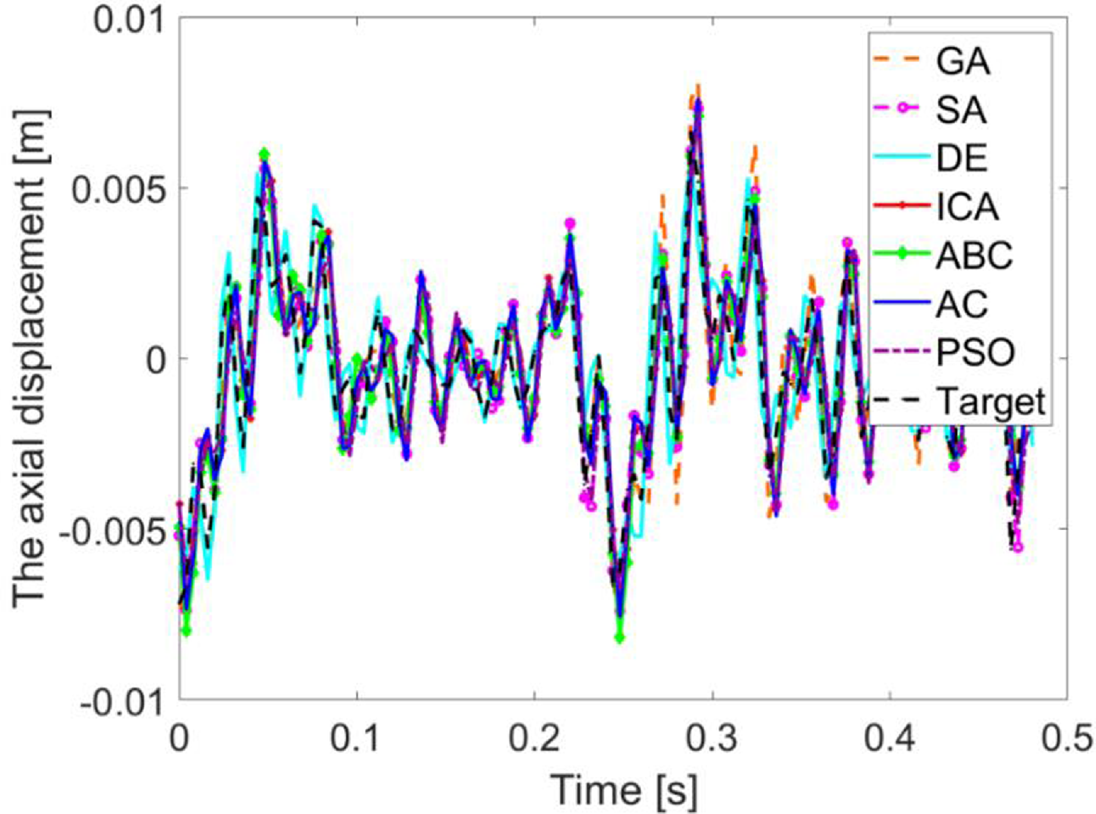
Figure 29. The flexible follower midpoint axial displacement.
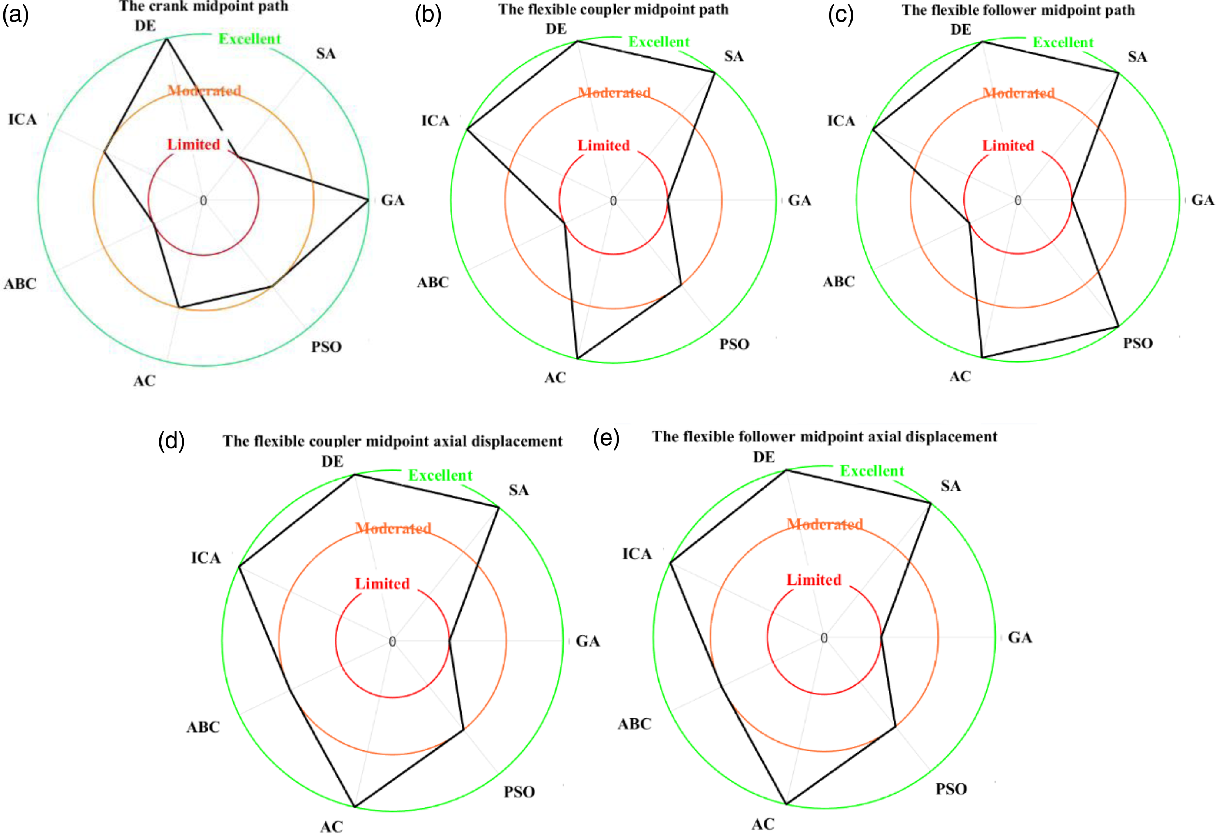
Figure 30. Graphical summary for the performance of the optimization techniques based on the combined synthesis, (a) for the crank midpoint path, (b) for the flexible coupler midpoint path, (c) for the flexible follower midpoint path, (d) for the flexible coupler midpoint axial displacement, and (e) for the flexible follower midpoint axial displacement.
In addition to the three aforementioned responses, the mechanism is subject to given axial displacement responses. Furthermore, controlling the axial displacement contributes to alleviate the flexible bodies’ impact on the mechanism response. Contrary to solid multibody systems, flexible bodies deviate the mechanism from its target response. Figures 28 and 29 represent the obtained results for the set of optimization techniques tested in this work. It can be observed that, apart from the ABC and GA, performances of other techniques remain acceptable. For the DE and AC techniques, the axial displacement responses almost overlap the target ones. Hence, the designer can consider the possibility of making the coupler or the follower midpoints’ part of another mechanism to build more complicated mechanical devices. The performance of each optimization technique based on the different responses has been assessed in Table VII and graphically summarized in Fig. 30.
Comparing the different optimization techniques for the four-bar mechanism synthesis reveals that some techniques could be appealing. It is worth mentioning that being more advantageous depends imperatively on the application type and design stage. For applications wherein the accuracy is a major concern, the trio SA, DE, and Ant Colony optimization are taking the lead. Despite being the technique managing to deplete the error to the lowest values, the SA requires more resources for the calculation time. The Ant Colony requires only 15% of the CPU time, whereas the DE requires 47% of the CPU time required by the SA. The increase of accuracy for the SA is 6% compared to the AC and 3% to the DE. The PSO, ICA, and ABC performances’ are relatively similar. Among the three aforementioned techniques, the ICA seems to be the most convenient as it offers the highest accuracy with the minimum CPU time. Even though the ABC technique has the advantage of providing design parameters with decent accuracy, its abundantly high CPU time is a major downside.
It can be confirmed from Appendix Table AV that the error values are within the same range of values as in refs. [Reference Ebrahimi and Payvandy4, Reference Zhang, Yang, Zhang and Huang58, Reference Rout and Mittal60, Reference Torres-Moreno, Cruz, Álvarez, Redondo and Giménez-Fernandez61]. This confirms the suitability of the proposed cost function by the authors to provide significant and meaningful results for the mechanism synthesis based on dynamic responses.
6. Conclusion
This work denotes an insight into flexible mechanisms synthesis. A flexible slider-crank and four-bar mechanisms have been used as illustrative examples. Six design variables have been of scope for the flexible slider-crank mechanism encompassing dimensional and material characteristics parameters. Whereas four dimensional parameters have been of interest for the flexible four-bar mechanism. Seven optimization techniques have been used for the mechanism synthesis based on either a dynamic response or axial displacement for flexible parts. Some important conclusions about the performance of the optimization techniques can be drawn. The ant colony and the DE techniques outstandingly perform compared to the other techniques for a single synthesis-based response. It should be highlighted that for flexible mechanisms, a single synthesis-based response satisfies only the response involved in the synthesis process. For the combined synthesis, all the responses involved are satisfied simultaneously concluding a perfect trade-off between them. The proposed approach offers to the designer a set of possible solutions for the synthesis problem based on noncommon responses, namely dynamic responses or a flexible link axial displacement. Moreover, the material characteristics such as Young modulus and material density are parts of the parameters to optimize. It is interesting to extend this work to other mechanisms such as robot arms and exoskeleton. Including clearance into the mechanical joints alongside flexible bodies is also of scope in future works.
Table VII. Summary of the synthesis results for the four-bar mechanism.
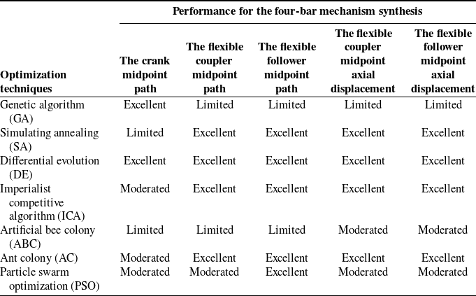
Author contributions
Mohamed Amine Ben Abdallah and Imed Khemili conceived and designed the study. Mohamed Amine Ben Abdallah conducted data gathering and analyses of the results and wrote the article. Imed Khemili, Nizar Aifaoui, and Med Amine Laribi reviewed the first draft of the manuscript.
Financial support
This research received no specific grant from any funding agency, commercial, or not-for-profit sectors.
Competing interests
The authors declare that there is no competing interests.
Appendix A

Figure A1. Histograms of the objective function computed in 100 runs of the slider velocity synthesis.
Table AI. Classification of the bibliographic references.
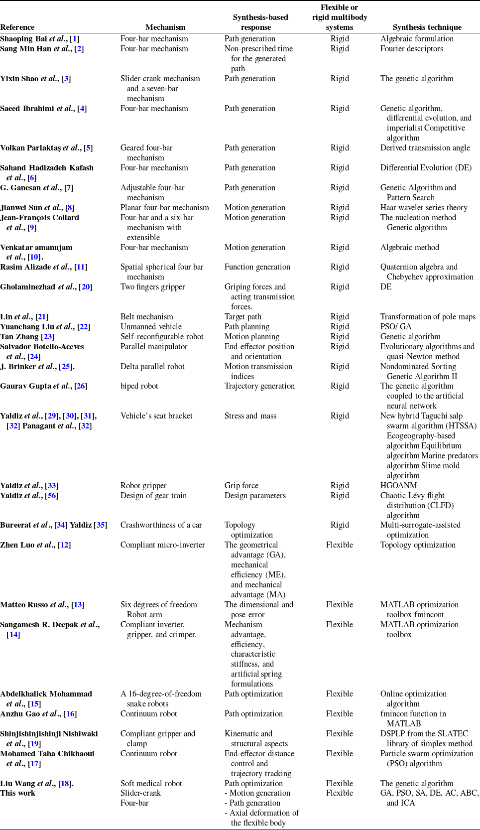

Figure A2. The automatic interaction between optimization module and dynamic analysis module for the Computer-Aided Design for Multibody Systems.
Table AII. The obtained mechanism design variables based on the slider velocity synthesis.


Figure A3. Histograms of the objective function computed in 100 runs of the axial displacement synthesis.
Table AIII. The obtained mechanism design variables based on the flexible connecting rod midpoint axial displacement.
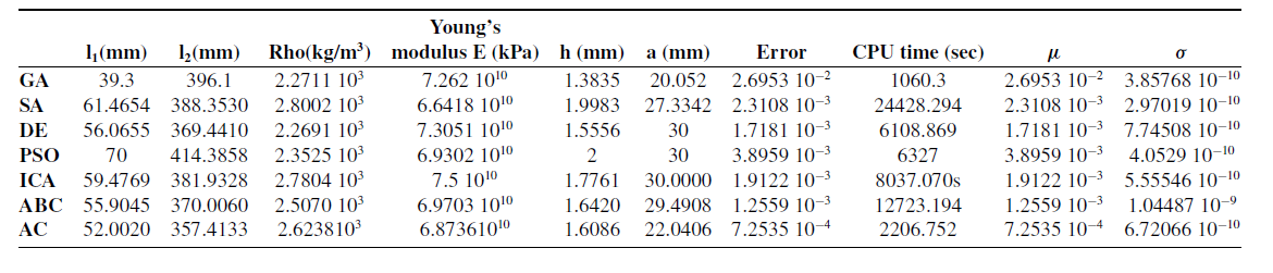

Figure A4. Histograms of the objective function computed in 100 runs of the combined synthesis.
Table AIV. The obtained mechanism design variables based on the combined synthesis.
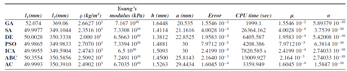
Table AV. The obtained results for the flexible four-bar mechanism based on the combined synthesis.

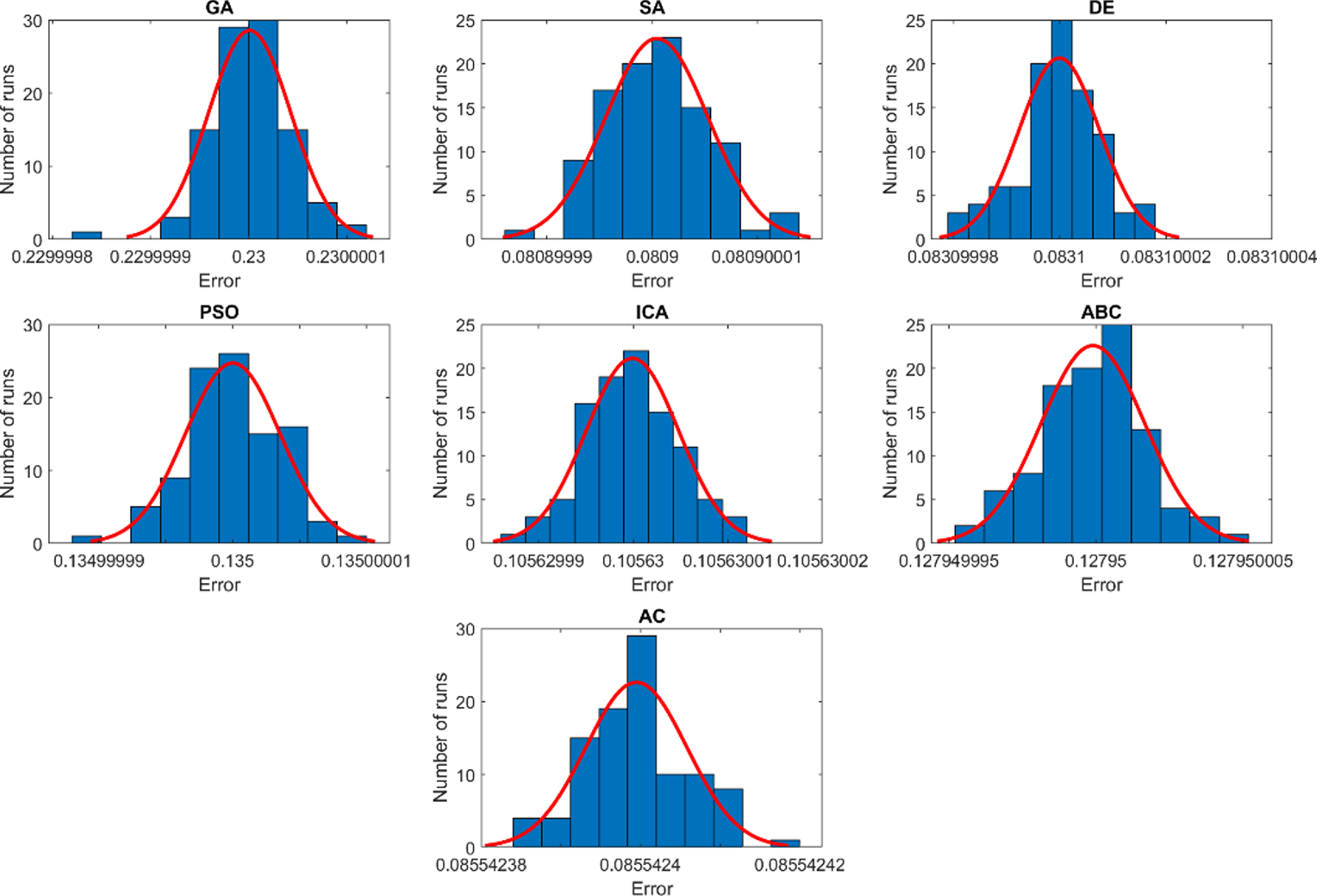
Figure A5. Histograms of the objective function computed in 100 runs for the flexible four-bar mechanism based on the combined synthesis.
Appendix B. Glossary.

Appendix C. List of abbreviations


 Open access