


1. Introduction
Gait trajectory prediction is a long-term research topic in human–machine interaction. Formally, gait trajectory prediction predicts the lower limb movement data based on certain types of sensor information collected currently (the movement data can be spatial position, angle, speed, and acceleration). It is an actual application of time-series forecasting techniques. Good gait prediction results can provide a necessary basis for the fields of lower limb exoskeleton control and human behavior prediction.
At time t, $X^{t} = \left \{ x_{1}^{t},\ldots,x_{L_{x}}^{t} | x_{i}^{t} \in R^{d_{x}} \right \}$
represents the input sensor data,
$X^{t} = \left \{ x_{1}^{t},\ldots,x_{L_{x}}^{t} | x_{i}^{t} \in R^{d_{x}} \right \}$
represents the input sensor data, $Y^{t} = \left \{ y_{1}^{t},\ldots,y_{L_{y}}^{t} | y_{i}^{t} \in R^{d_{y}} \right \}$
represents the output forecast data, where
$Y^{t} = \left \{ y_{1}^{t},\ldots,y_{L_{y}}^{t} | y_{i}^{t} \in R^{d_{y}} \right \}$
represents the output forecast data, where $L_y$
and
$L_y$
and $L_x$
are the lengths of the predicted sequence and the input sequence, respectively, and
$L_x$
are the lengths of the predicted sequence and the input sequence, respectively, and $d_y$
and
$d_y$
and $d_x$
are the dimensions of the predicted sequence and the input sequence, respectively.
$d_x$
are the dimensions of the predicted sequence and the input sequence, respectively.
At present, the deep neural network is the primary method used to predict the gait trajectory, but there are three primary deficiencies in the current research:
-
1. At present, most of the neural network models used for gait prediction only predict the gait trajectory of dozens or even only a few time frames in the future. A too-short prediction window will result in a significant time interval of the predicted trajectory or a short prediction time, which limits the application of the prediction results. For example, short-term gait prediction cannot effectively assist the control of the lower extremity exoskeleton because of motor output delay.
-
2. Currently, almost no neural network models with high accuracy used for gait prediction are interpretable. Although these models can somewhat predict the future gait trajectory, they are black boxes. The non-interpretable neural network model used for gait prediction cannot provide a further reference for gait research.
Long-term series forecasting refers to time-series forecasting with an enormous value of $L_{y}$
. There is no clear threshold to define long-term series forecasting, but the value of
$L_{y}$
. There is no clear threshold to define long-term series forecasting, but the value of $L_{y}$
generally needs to be in the hundreds (Fig. 1).
$L_{y}$
generally needs to be in the hundreds (Fig. 1).
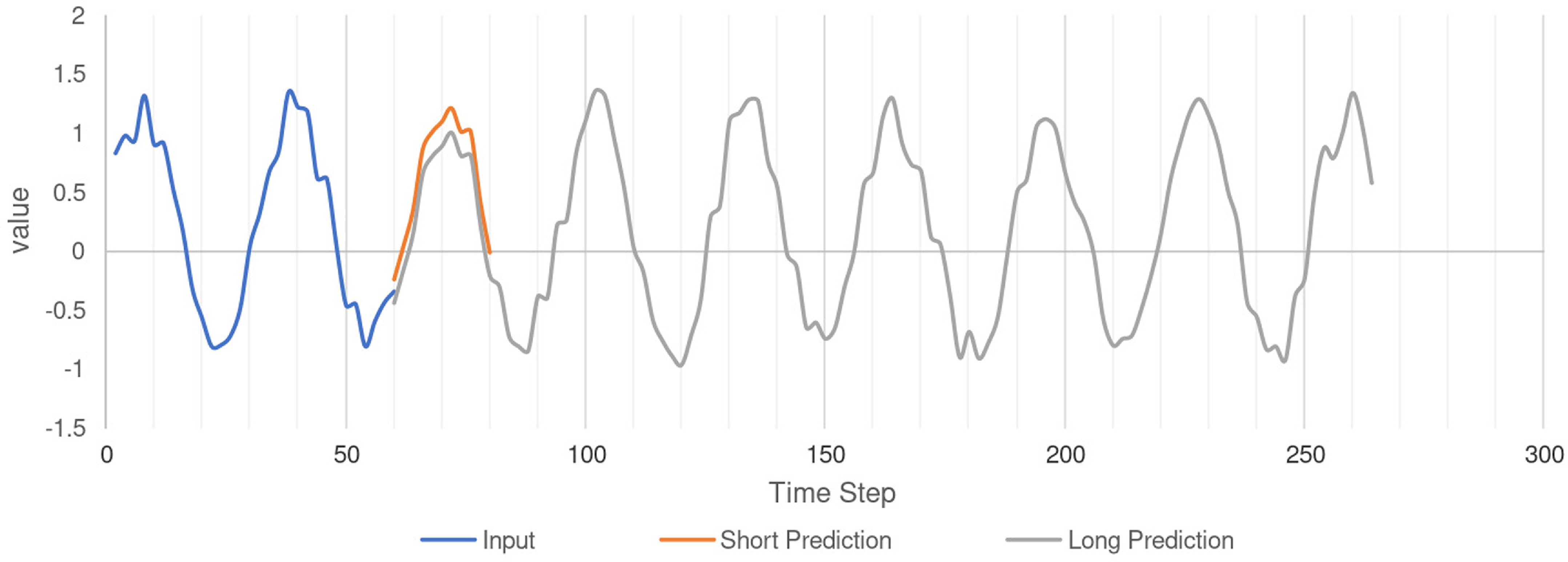
Figure 1. Long-term series forecasting.
Based on the above insights, we propose the Interpretable-Concatenation former (IC-former) model, which can interpretably predict long-term gait trajectories by quantifying the importance of data from different segments of the input sequence. The model is built according to the encoder–decoder structure using the dot-product attention mechanism. The IC-former model generatively outputs long-term forecast sequences, which avoids errors caused by cyclic calculations like the RNN model and speeds up calculations. The interpretive network can help people understand the model’s logic, formulate control strategies, and assist in medical diagnosis. The framework structure of the IC-former model is shown in Fig. 2. The main contributions of this paper are as follows:
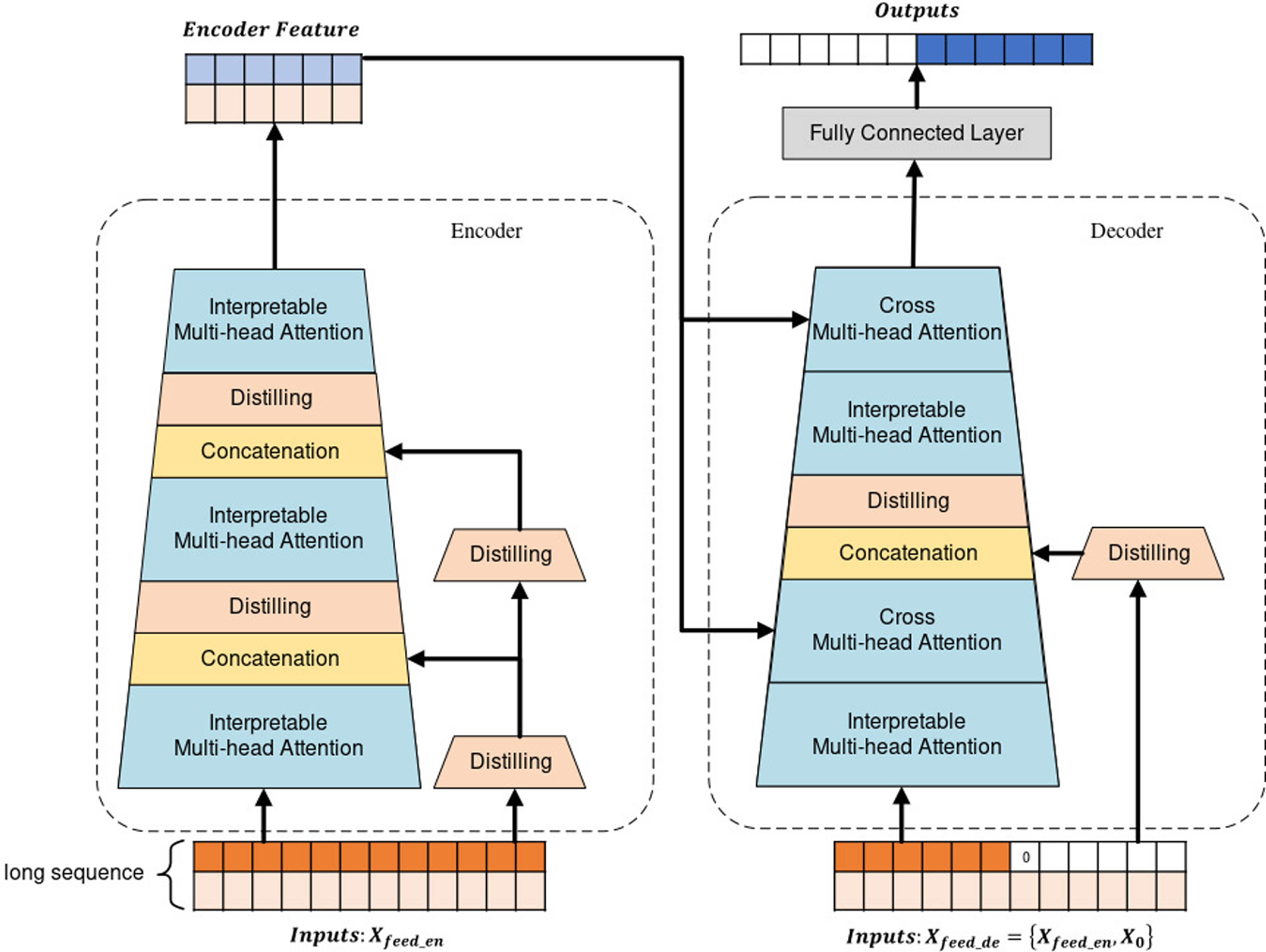
Figure 2. Interpretable Multi-head Attention is an interpretable dot-product attention layer proposed by us, whose attention value can measure the importance of the input. The distilling layers are 1D convolutional layers, halving the data length and efficiently extracting context-related features. The Concatenation operation merges the data features of parallel channels to add features with explicit meaning to the main channel. The encoder receives a long sequence and then feeds it into two parallel channels. The main channel contains Interpretable Multi-head Attention, through which the IC-former model extracts the main feature. The other channel is the auxiliary channel, which has distilling layers that preserve the mathematical meaning of the input. There are two differences between the decoder and the encoder. The first difference is that the decoder receives a long sequence of inputs, and pads target elements with zeros. Another difference is that the decoder contains Cross Multi-head Attention to combine the extracted features from the encoder and decoder. Finally, the decoder immediately predicts output elements in a generative style.
-
1. The proposed IC-former model can accurately predict long-term gait trajectories. It can generate long-term prediction sequences based on one-time input, reducing the cumulative calculation error. The model provides a good reference for formulating lower extremity exoskeleton control strategies and predicting human behavior.
-
2. Unlike previous black boxes, the proposed IC-former is an interpretive network relying on the dot-product attention mechanism, which can locate the critical parts of the gait trajectory.
-
3. The prediction accuracy of the IC-former is higher than that of a series of time-series prediction models widely used in gait trajectory prediction. In the case of the same length of the input sequence, the scale of the IC-former is smaller than that of the Informer model, which is more suitable for application on mobile computing platforms.
2. Related work
2.1. Gait trajectory prediction
Traditional gait prediction methods represented by controlled oscillators can deal with some simple fixed-period gait prediction problems. Adaptive oscillators can predict cyclic and quasi-cyclic gait sequences., but they cannot predict rapidly changing gaits in time. The traditional gait prediction method has a noticeable delay in predicting rapidly changing gait. This shortcoming limits the application of the traditional method [Reference Xue, Wang, Zhang and Zhang1, Reference Seo, Kim, Park, Cho, Lee, Choi, Lim, Lee and Shim2].
The data-based deep learning method can directly output the trajectory in the future based on the sensor data without an iterative update of parameters, which solves the delay problem. Tanghe et al. and Kang et al. predicted the gait phase [Reference Tanghe, De Groote, Lefeber, De Schutter and Aertbeliën3, Reference Kang, Kunapuli and Young4] based on the deep neural network, but their models had high requirements for the type and quantity of sensors, and the workload of processing data was heavy. High requirements limit the real-world application of their method. It is significant to reduce the type and quantity of sensors as much as possible to reduce the cost of gait prediction.
As an important method for processing sequence information, the long short-term memory (LSTM) model is widely used to predict gait trajectory [Reference Wang, Li, Wang, Yu, Liao and Arifoglu5, Reference Zaroug, Garofolini, Lai, Mudie and Begg6, Reference Zaroug, Lai, Mudie and Begg7, Reference Su and Gutierrez-Farewik8, Reference Liu, Wu, Wang and Chen9]. These models can only predict gait trajectories within a limited time frame. When predicting long-term gait trajectories, the LSTM model they adopted is slow and has a large cumulative error caused by the loop structure of the LSTM model itself.
Karakish et al. and Kang et al. used a CNN-based deep neural network to predict gait [Reference Karakish, Fouz and ELsawaf10, Reference Kang, Molinaro, Duggal, Chen, Kunapuli and Young11], which is faster than the LSTM model. However, the model proposed by Karakish et al. can only predict the gait trajectory in a short time, and the model proposed by Kang et al. relies on user-specific basis data.
The gait trajectory prediction models mentioned above are difficult to predict long-term gait trajectory, and none of them consider the issue of model interpretability. They cannot judge the input’s importance or explain the model’s data basis. The above models only predict gait as a black box and cannot support in-depth gait research.
2.2. Long-term series forecasting
Currently, in the time-series forecasting field, one challenging work is improving the performance of long sequence time-series forecasting (LSTF). Predicting long-period gait is more difficult than predicting short-period gait. It can explore the deep-level characteristics of gait data and help people design more optimal control strategies.
Before the Transformer structure was developed, recurrent neural network (RNN) models dominated time-series forecasting [Reference Cao, Li and Li12, Reference Sagheer and Kotb13, Reference Sagheer and Kotb14]. Hochreiter et al. propose a LSTM model for solving the gradient vanishing issues [Reference Hochreiter and Schmidhuber15]. Although the LSTM model is excellent, the low computational efficiency brought about by its cyclic structure and the difficulty of feature extraction when dealing with long sequences limit its application.
Since the Transformer model was proposed in the field of natural language processing [Reference Vaswani, Shazeer, Parmar, Uszkoreit, Jones, Gomez, Kaiser and Polosukhin16], its ability to process sequence data has been applied to predict time series [Reference Zerveas, Jayaraman, Patel, Bhamidipaty and Eickhoff17, Reference Xu, Dai, Liu, Gao, Lin, Qi and Xiong18]. Although the Transformer model has brought many breakthroughs, it is expensive to use the self-attention mechanism directly in LSTF because of its L-quadratic memory and computation consumption on L-length inputs/outputs. Many improvements are proposed to solve this problem [Reference Kitaev, Kaiser and Levskaya19, Reference Wang, Li, Khabsa, Fang and Ma20]. Li et al. present LogSparse Transformer which the memory cost of the self-attention mechanism is only $O\left ({L*\left ({log(L)} \right )^{2}} \right )$
[Reference Li, Jin, Xuan, Zhou, Chen, Wang and Yan21]. Beltagy et al. introduce an attention mechanism called Longformer that scales linearly with sequence length, reducing its complexity to
$O\left ({L*\left ({log(L)} \right )^{2}} \right )$
[Reference Li, Jin, Xuan, Zhou, Chen, Wang and Yan21]. Beltagy et al. introduce an attention mechanism called Longformer that scales linearly with sequence length, reducing its complexity to $O\left ({L*log(L)} \right )$
[Reference Beltagy, Peters and Cohan22]. A representative example of all relevant improvements is the Informer model proposed by Zhou et al., which predicts the output more quickly and accurately with less memory and computation consumption than previous methods [Reference Zhou, Zhang, Peng, Zhang, Li, Xiong and Zhang23]. The Informer model has one essential breakthrough: the ProbSparse self-attention mechanism.
$O\left ({L*log(L)} \right )$
[Reference Beltagy, Peters and Cohan22]. A representative example of all relevant improvements is the Informer model proposed by Zhou et al., which predicts the output more quickly and accurately with less memory and computation consumption than previous methods [Reference Zhou, Zhang, Peng, Zhang, Li, Xiong and Zhang23]. The Informer model has one essential breakthrough: the ProbSparse self-attention mechanism.
The above time-series forecasting models significantly reduced the model size and improved forecasting accuracy. However, none is interpretable. Prediction accuracy also needs to be improved.
2.3. Model interpretability
The current methods of interpreting neural networks are mainly divided into gradient-based methods and methods based on adjusting input values [Reference Chen, Song, Wainwright and Jordan24]. The attention mechanism of a neural network multiplies the input with nonzero weights that sum to 1. The attention weight of a variable perceptually represents the importance of the variable. Research on the interpretation of neural networks proves that the value of the attention of the Transformer structure is indeed positively correlated with the importance of variables [Reference Jain and Wallace25, Reference Vig and Belinkov26, Reference Vashishth, Upadhyay, Tomar and Faruqui27]. Many interpretable neural network models for time-series forecasting have been proposed. Oreshkin et al. proposed an interpretable time-series forecasting model named N-BEATS, but it can only predict the time series of a dozen time frames in the future, which cannot meet the needs of long-term series forecasting [Reference Oreshkin, Carpov, Chapados and Bengio28]. Lim et al. proposed Temporal Fusion Transformers, a time-series prediction model that combines LSTM and Transformer structures. The LSTM framework it uses limits its application to predicting long-term series [Reference Lim, Arık, Loeff and Pfister29]. In summary, studying interpretable neural network models for long-term series forecasting is meaningful.
3. Interpretable-Concatenation former
The Transformer model based on the dot-product attention mechanism can effectively extract the data features of sequence information. However, to improve efficiency and accuracy, the Transformer model breaks the mathematical meaning of the input variables. The breaking mathematical meaning makes the Transformer model an uninterpretable black box. A critical issue is how to preserve the mathematical meaning of the input variables with high accuracy and efficiency. Studying this problem is of great significance to studying the interpretability of neural network models, especially Transformer models.
Driven by the above ideas, we propose Interpretable Multi-head Attention, which adjusts the traditional Transformer structure to retain the clear mathematical meaning of the input and ensures that only the weight-adjusted input determines the output. Therefore, the weight calculated by Interpretable Multi-head Attention can measure the importance of the mathematical meaning represented by different input fragments. Further, we propose the IC-former model based on Interpretable Multi-head Attention. IC-former is a deep neural network model of the encoder–decoder structure. IC-former can measure the importance of inputs of different lengths at different locations on both local and global scales with high predicting accuracy. The IC-former model generatively outputs long-term forecast sequences, which makes the model calculation fast and eliminates cumulative errors. The IC-former model is shown in Fig. 3.

Figure 3. 1: Distilling layer; 2: Concatenation operation; 3: Interpretable Multi-head Attention layer; 4: Cross Multi-head Attention layer; 5: Interpretable-Concatenation former.
3.1. Attention mechanisms
Ashish et al. propose the Transformer based solely on attention mechanisms. The Transformer uses stacked self-attention and point-wise, fully connected layers for both the encoder and decoder to form an encoder–decoder structure.
The core of the attention mechanism is the scaled dot-product attention. Calculating the scaled dot-product attention requires three parameters: queries $(Q)$
, keys
$(Q)$
, keys $(K)$
, and values
$(K)$
, and values $(V)$
, where
$(V)$
, where $Q \in R^{L_{Q}*d}$
,
$Q \in R^{L_{Q}*d}$
, $K \in R^{L_{K}*d}$
,
$K \in R^{L_{K}*d}$
, $V \in R^{L_{V}*d}$
, and d is the input dimension. The formula is Eq. (1):
$V \in R^{L_{V}*d}$
, and d is the input dimension. The formula is Eq. (1):
 \begin{equation} Attention\left ({Q,K,V} \right ) = softmax\left ( \frac{Q*K^{T}}{\sqrt{d}} \right )*V \end{equation}
The Transformer can be trained significantly faster than architectures based on recurrent or convolutional layers and outperforms them for translation tasks. The attention mechanism effectively splits the input space, emphasizing only elements relevant to the task. Transformer structure is widely used in text-based and chart-based tasks because of its robust feature extraction ability to sequences.
3.2. Informer
Dot-product attention mechanisms require calculating each dot-product pair, which makes the computational cost of the attention mechanism increase squarely with the linear increase of the sequence length $\left ( L_{Q}, L_{K} \right )$
. This property makes long-term series forecasting expensive in computation. To solve this problem, Haoyi et al. propose ProbSparse Self-attention and apply it to the Informer model. They propose the Query Sparsity Measurement to find the most critical vectors of queries
$\left ( L_{Q}, L_{K} \right )$
. This property makes long-term series forecasting expensive in computation. To solve this problem, Haoyi et al. propose ProbSparse Self-attention and apply it to the Informer model. They propose the Query Sparsity Measurement to find the most critical vectors of queries $(Q)$
. The formula is Eq. (2), where
$(Q)$
. The formula is Eq. (2), where $L_{K}$
represents the length of
$L_{K}$
represents the length of $K$
,
$K$
, $d$
represents the model dimension, and
$d$
represents the model dimension, and $q_i$
,
$q_i$
, $k_i$
, and
$k_i$
, and $v_i$
are the
$v_i$
are the $i$
th row in
$i$
th row in $Q$
,
$Q$
, $K$
, and
$K$
, and $V$
, respectively:
$V$
, respectively:
 \begin{equation} M\left ({q_{i},K} \right ) = ln{\sum \limits _{j = 1}^{L_{K}}e^{\frac{q_{i}*{k_{j}}^{T}}{\sqrt{d}}}} - \frac{1}{L_{K}}{\sum \limits _{j = 1}^{L_{K}}\frac{q_{i}*{k_{j}}^{T}}{\sqrt{d}}} \end{equation}
Query Sparsity Measurement is Kullback–Leibler divergence between $q_{i}$
and
$q_{i}$
and $K$
. The larger the Query Sparsity Measurement is, the more different
$K$
. The larger the Query Sparsity Measurement is, the more different $q_{i}$
and
$q_{i}$
and $K$
are, and the more critical
$K$
are, and the more critical $q_{i}$
is. Based on the Query Sparsity Measurement, the ProbSparse Self-attention allows each
$q_{i}$
is. Based on the Query Sparsity Measurement, the ProbSparse Self-attention allows each $K$
only to attend to the
$K$
only to attend to the $u$
-dominant
$u$
-dominant $q_{i}$
. The formula is Eq. (3):
$q_{i}$
. The formula is Eq. (3):
 \begin{equation} Attention\left ({Q,K,V} \right ) = softmax\left ( \frac{\overline{Q}*K^{T}}{\sqrt{d}} \right )*V \end{equation} $\overline{Q}$
is a sparse matrix only containing the top-
$\overline{Q}$
is a sparse matrix only containing the top- $u$
vectors of
$u$
vectors of $Q$
measured by the Query Sparsity Measurement.
$Q$
measured by the Query Sparsity Measurement. $u\,=\,c\,\cdot \,ln\,L_{Q}$
where
$u\,=\,c\,\cdot \,ln\,L_{Q}$
where $c$
is a constant sampling factor. Then, the ProbSparse Self-attention only calculates
$c$
is a constant sampling factor. Then, the ProbSparse Self-attention only calculates $O\left ( ln\,L_{Q} \right )$
dot-product for each query-key pair, and the layer memory usage is reduced to
$O\left ( ln\,L_{Q} \right )$
dot-product for each query-key pair, and the layer memory usage is reduced to $O\left ( L_{K}\,ln\,L_{Q} \right )$
. For self-attention
$O\left ( L_{K}\,ln\,L_{Q} \right )$
. For self-attention $ L_{Q} = L_{K} = L$
, so the complexity and space complexity of the ProbSparse self-attention is
$ L_{Q} = L_{K} = L$
, so the complexity and space complexity of the ProbSparse self-attention is $O(L\,ln\,L)$
.
$O(L\,ln\,L)$
.
Informer adopts the self-attention distilling mechanism, adding a convolutional layer on the time dimension between the attention modules. A max-pooling layer with two strides is added to down-sample inputs into its half slice. The distilling mechanism reduces memory usage to $O\left ( (2\, - \epsilon )L\,log\,L \right )$
while ensuring computational accuracy.
$O\left ( (2\, - \epsilon )L\,log\,L \right )$
while ensuring computational accuracy.
3.3. Distilling layer
The distilling layer is a 1D convolutional layer whose output sequence’s length is half the length of the input sequence. The distilling layer reduces the sequence length, memory consumption, and computational complexity. It is also possible to further reduce the sequence length to a quarter or less, which needs to be determined according to the prediction accuracy and scale of the model. Finding the sequence segment with the most information is crucial for interpreting the gait trajectory prediction model. In this paper, we focus on methods to measure the importance of the temporal dimension. So we choose a one-dimensional convolutional network instead of a two-dimensional convolutional network:
 \begin{equation}{C_{dis}}_{\frac{L}{2} \times d} ={Conv1d}_{C}\left ( C_{L \times d} \right )\,\,\,\,\,\,\,\,C_{L \times d} \in \left \{{Q,K,V} \right \} \end{equation}
The distilling layer in the IC-former model has three important functions:
-
1. The distilling layers reduce the length of the input to half, significantly reducing the model size. Reducing model size is especially important when the input and predicted sequences are long.
-
2. The distilling layers effectively extract context-related features, which helps to improve the prediction accuracy of the model.
-
3. The distilling layers retain the mathematical meaning of the input. The convolutional network’s local calculation characteristics make the model’s calculation process easier for humans to understand.
3.4. Concatenation operation
The Concatenation operation is an operation that splices two pieces of data together in the time dimension. It is worth noting that there are Concatenation operations inside and outside the attention layer of the IC-former model. Concatenation operations play different roles inside and outside the attention layer:
 \begin{equation} A_{cat} = \mathbf{C}\mathbf{o}\mathbf{n}\mathbf{c}\mathbf{a}\mathbf{t}\mathbf{e}\mathbf{n}\mathbf{a}\mathbf{t}\mathbf{i}\mathbf{o}\mathbf{n}\left \{ \left ({Input_A,Input_B} \right )\!,\mathbf{d}\mathbf{i}\mathbf{m} = \mathbf{t}\mathbf{i}\mathbf{m}\mathbf{e} \right \} \end{equation}
The function of the Concatenation operation inside the attention layer is to splice the process variable queries (Q) with the original attention. It enables queries (Q) to continue participating in subsequent calculations as primary features instead of being discarded directly, breaking the original barriers between data. Concatenation operation outside the attention layer splices the auxiliary and main channels in the time dimension to obtain the concatenated information. The attention calculated for the concatenated information represents the relative importance of each input segment.
3.5. Interpretable Multi-head Attention
Although the traditional Transformer structure has proved its powerful feature extraction ability, it destroys the mathematical meaning of the data. The Transformer model cannot measure the data’s importance because of the following two reasons: 1: The queries $(Q)$
, keys
$(Q)$
, keys $(K)$
, and values
$(K)$
, and values $(V)$
in the traditional Transformer structure are obtained by the fully connected layer. But the fully connected layer directly destroys its mathematical meaning. 2: The traditional Transformer structure adds the output of dot-product attention with its original input at the element level, which keeps the original data features. However, it also causes the original data features to continue participating in the subsequent calculation process without being adjusted by the attention weight. The addition at the element level also confuses the mathematical meaning of the data.
$(V)$
in the traditional Transformer structure are obtained by the fully connected layer. But the fully connected layer directly destroys its mathematical meaning. 2: The traditional Transformer structure adds the output of dot-product attention with its original input at the element level, which keeps the original data features. However, it also causes the original data features to continue participating in the subsequent calculation process without being adjusted by the attention weight. The addition at the element level also confuses the mathematical meaning of the data.
In response to these two points, we made adjustments and proposed Interpretable Multi-head Attention. There are two main improvements of Interpretable Multi-head Attention:
-
1. Get queries $(Q)$
, keys
$(K)$
, and values
$(V)$
through the distilling layer, which has three advantages. The characteristics of the local calculation of the convolutional network ensure that the mathematical meaning of the obtained queries
$(Q)$
, keys
$(K)$
, and values
$(V)$
is clear and can be intuitively understood by humans. The convolutional network is suitable and efficient for processing sequence information. The data length of queries
$(Q)$
, keys
$(K)$
, and values
$(V)$
obtained by the distilling layer is half of the input, reducing the model’s memory usage.
$(Q)$
, keys
$(K)$
, and values
$(V)$
through the distilling layer, which has three advantages. The characteristics of the local calculation of the convolutional network ensure that the mathematical meaning of the obtained queries
$(Q)$
, keys
$(K)$
, and values
$(V)$
is clear and can be intuitively understood by humans. The convolutional network is suitable and efficient for processing sequence information. The data length of queries
$(Q)$
, keys
$(K)$
, and values
$(V)$
obtained by the distilling layer is half of the input, reducing the model’s memory usage. -
2. Interpretable Multi-head Attention no longer adds the original input to the output of the attention mechanism at the element level, which ensures that all the data features of the model are obtained based on the weight-adjusted data.


Each column of the attention weight matrix represents the importance of the data corresponding to each row of values $(V)$
. The weight matrix of the attention mechanism calculated by queries
$(V)$
. The weight matrix of the attention mechanism calculated by queries $(Q)$
and keys
$(Q)$
and keys $(K)$
is represented by W, and the elements of each matrix are represented by lowercase letters. L is the length of the input sequence, and d is the model dimension:
$(K)$
is represented by W, and the elements of each matrix are represented by lowercase letters. L is the length of the input sequence, and d is the model dimension:
 \begin{equation} W\, = \,Q\,*\,K = \left[\begin{array}{c@{\quad}c@{\quad}c} w_{1,1} & \cdots & w_{1,L} \\[5pt] \vdots & \ddots & \vdots \\[5pt] w_{L,1} & \cdots & w_{L,L} \end{array}\right] \end{equation}
 \begin{align} A &= \,W\,*\,V = \left[\begin{array}{c@{\quad}c@{\quad}c} w_{1,1} & \cdots & w_{1,L} \\[5pt] \vdots & \ddots & \vdots \\[5pt] w_{L,1} & \cdots & w_{L,L} \end{array}\right]\ast \left[\begin{array}{c@{\quad}c@{\quad}c} v_{1,1} & \cdots & v_{1,d} \\[5pt] \vdots & \ddots & \vdots \\[5pt] v_{L,1} & \cdots & v_{L,d} \end{array}\right]\nonumber \\[5pt] &= \left[\begin{array}{c@{\quad}c@{\quad}c} {w_{1,1}*v_{1,1} + \ldots + w_{1,L}*v_{L,1}} & \cdots &{w_{1,1}*v_{1,d} + \ldots + w_{1,L}*v_{L,d}} \\[5pt] \vdots & \ddots & \vdots \\[5pt] {w_{L,1}*v_{1,1} + \ldots + w_{L,L}*v_{L,1}} & \cdots & w_{L,1}*v_{1,d} + \ldots + w_{L,L}*v_{L,d} \end{array}\right] \end{align}
The multi-head attention mechanism divides the data’s model dimension into multiple modules, which does not destroy the mathematical meaning of the 1D convolutional layer. The attention of the whole model dimension is the summing of all multi-head attention. Let H denote the total number of heads, and h represents the hth head:
 \begin{equation} W^{h}\, = \,Q^{h}\,*\,K^{h} = \left[\begin{array}{c@{\quad}c@{\quad}c} {w_{1,1}}^{h} & \cdots &{w_{1,L}}^{h} \\[5pt] \vdots & \ddots & \vdots \\[5pt] {w_{L,1}}^{h} & \cdots &{w_{L,L}}^{h} \end{array} \right]\end{equation}
 \begin{equation} \begin{split} A^{h}\, = \,W^{h}\,*\,V^{h}\, = \begin{bmatrix}{w_{1,1}}^{h}\;\;\;\;\; & \cdots\;\;\;\;\; &{w_{1,L}}^{h} \\[5pt] \vdots\;\;\;\;\; & \ddots\;\;\;\;\; & \vdots \\[5pt] {w_{L,1}}^{h}\;\;\;\;\; & \cdots\;\;\;\;\; &{w_{L,L}}^{h} \\[5pt] \end{bmatrix}*\begin{bmatrix}{v_{1,1}}^{h}\;\;\;\;\; & \cdots\;\;\;\;\; &{v_{1,d/H}}^{h} \\[5pt] \vdots\;\;\;\;\; & \ddots\;\;\;\;\; & \vdots \\[5pt] {v_{L,1}}^{h}\;\;\;\;\; & \cdots\;\;\;\;\; &{v_{L,d/H}}^{h} \\[5pt] \end{bmatrix} \\[5pt] = \,\begin{bmatrix}{{w_{1,1}}^{h}*{v_{1,1}}^{h} + \ldots +{w_{1,L}}^{h}*{v_{L,1}}^{h}}\;\;\;\;\; & \cdots\;\;\;\;\; &{{w_{1,1}}^{h}*{v_{1,d/H}}^{h} + \ldots +{w_{1,L}}^{h}*{v_{L,d/H}}^{h}} \\[5pt] \vdots\;\;\;\;\; & \ddots\;\;\;\;\; & \vdots \\[5pt] {{w_{L,1}}^{h}*{v_{1,1}}^{h} + \ldots +{w_{L,L}}^{h}*{v_{L,1}}^{h}}\;\;\;\;\; & \cdots\;\;\;\;\; &{{w_{L,1}}^{h}*{v_{1,d/H}}^{h} + \ldots +{w_{L,L}}^{h}*{v_{L,d/H}}^{h}} \\[5pt] \end{bmatrix} \end{split} \end{equation}
 \begin{equation} W\, = \,{\sum \limits _{h = 1}^{h = H}W^{h}} \end{equation}
To further reduce the computational complexity and memory consumption, we use the ProbSparse attention proposed in [Reference Zhou, Zhang, Peng, Zhang, Li, Xiong and Zhang23] to replace the traditional dot-product attention.
3.6. Cross Multi-head Attention
The basic structure of Cross Multi-head Attention is similar to that of Interpretable Multi-head Attention. They both use the distilling layer and Concatenation operations. There are only two differences between them. In the Cross Multi-Head Attention, keys $ (k)$
and values
$ (k)$
and values $ (v)$
are calculated by the encoder feature and queries
$ (v)$
are calculated by the encoder feature and queries $ (q)$
are calculated by the decoder feature. Cross Multi-head Attention retains the addition of the input and output of the attention mechanism at the element level. Cross Multi-head Attention effectively fuses the features of the encoder and decoder.
$ (q)$
are calculated by the decoder feature. Cross Multi-head Attention retains the addition of the input and output of the attention mechanism at the element level. Cross Multi-head Attention effectively fuses the features of the encoder and decoder.
3.7. Encoder and decoder
The IC-former model is of an encoder–decoder structure. The encoder and decoder are obtained by repeatedly stacking the basic modules mentioned above according to the relationship shown in Fig. 3. The number of stacked modules can be flexibly adjusted based on data volume and model size.
We denote the length of the input sequence by L. The larger the value of L, the greater the consumption. This shortcoming is especially serious for dot-product attention because of L-quadratic memory and computation consumption on L-length inputs/outputs. To alleviate this problem, we use distilling layers in the attention layer and the encoder and decoder further to reduce the memory and computation consumption of the model.
The encoder and the decoder have two channels: main and auxiliary channels. The main channel measures the importance of the input sequence. The auxiliary channel provides the input with a precise mathematical meaning. Because the auxiliary channel only contains distilling layers, the data it processes retain a clear mathematical meaning. A Concatenation operation between the encoder and decoder concatenates the uninterpretable main channel and the interpretable auxiliary channel to obtain spliced features. The spliced features are input to the next module’s Interpretable Multi-head Attention module, and each fragment’s importance is measured. The attention of the interpretable auxiliary channel represents the relative richness of information in each sequence segment. The importance of the interpretable auxiliary channel features is also global, indicating the relative information abundance of each sequence segment in the model.
After the sequence passes through the stacked distilling layers in the auxiliary channel, the sequence length is shortened layer by layer. The granularity of the sequence continues to increase, which means that the length of the original input sequence represented by each vector increases accordingly. IC-former compares the relative importance of each fragment at different granularities. Measuring the local and global importance of sequence fragments reveals the data basis of the neural network model.
The structure of the decoder and the encoder is similar. The main difference is that the decoder has a Cross Multi-head Attention module, which fuses the features of the encoder and decoder. The input to the encoder is the entire input sequence. The input to the decoder is a combined sequence obtained by concatenating the input sequence and a zero sequence with the same length as the output sequence. The final decoder feature is input to a fully connected layer to obtain the final prediction output.
4. Experiment
4.1. Accuracy test
4.1.1. Datasets
We conduct experiments on datasets consistent with the Informer model to verify the prediction accuracy of our proposed IC-former model, in which the ETT dataset is collected by Zhou et al., and ECL and Weather are public benchmark datasets.
ETT (Electricity Transformer Temperature): ETT is a key indicator of the long-term deployment of electricity. The dataset records 2 years of data collected from two counties in China. To study the effect of granularity on the LSTF problem, the dataset contains 1-hour-level sub-datasets ETTh1 and ETTh2 and 15-minute-level sub-dataset ETTm1. Each data point has a target value, “oil temperature,” and six power load characteristics. Training/validation/testing is 12/4/4 months.
ECL (Electricity Consuming Load): It collects electricity usage (Kwh) from 321 customers. Like Zhou et al., we transformed the dataset into hourly consumption for 2 years. Training/validation/testing is 15/3/4 months
Weather: The dataset contains local climate data for nearly 1,600 locations in the United States, with data points collected every hour for 4 years from 2010 to 2013. Each data point has a “wet bulb” target value and 11 climate features. Training/validation/testing is 28/10/10 months.
4.1.2. Experimental details
Baselines: Zhou et al. tested Informer [Reference Zhou, Zhang, Peng, Zhang, Li, Xiong and Zhang30], ARIMA [Reference Ariyo, Adewumi and Ayo31], Prophet [Reference Taylor and Letham32], LSTMa [Reference Bahdanau, Cho and Bengio33], LSTnet [Reference Lai, Chang, Yang and Liu34], and DeepAR [Reference Salinas, Flunkert, Gasthaus and Januschowski35] on the above-mentioned datasets. We cite Zhou et al.’s experimental results to compare with those obtained by our proposed IC-former on the above datasets.
Although our proposed model can effectively multivariate and univariate forecasting, we focus on univariate forecasting. We believe predicting gait trajectory should depend on as few sensors as possible. Fewer sensors mean fewer hardware requirements, which can significantly reduce the application threshold of algorithms. In the part of experiments, the IC-former model contains a three-layer encoder and a two-layer decoder. In the other part of the experiments, the IC-former model includes a two-layer encoder and a one-layer decoder. The IC-former model is optimized with Adam optimizer, and its learning rate starts from 0.0001, decaying two times smaller every two epochs, and the total epochs are 20. We set the batch size to 32.
We used two evaluation metrics, $MSE$
and
$MSE$
and $MAE$
, on each prediction window (averaging for multivariate prediction) and rolled the whole set with
$MAE$
, on each prediction window (averaging for multivariate prediction) and rolled the whole set with $stride = 1$
:
$stride = 1$
:
 \begin{equation*} MSE=\frac {1}{n}\sum _{i=1}^{n}\left (y-\hat {y}\right )^2 \end{equation*}
 \begin{equation*} MAE=\frac {1}{n}\sum _{i=1}^{n}\left |y-\hat {y}\right | \end{equation*}
The prediction window sizes in ETTH, ECL, and Weather are $\left \{1d,2d,7d,14d,30d,40d\right \}$
. The prediction window size in ETTm is
$\left \{1d,2d,7d,14d,30d,40d\right \}$
. The prediction window size in ETTm is $\left \{6h,12h,24h,72h,168h\right \}$
. Our computing platform (Nvidia 3090 24 GB GPU) is a little worse than the platform (Nvidia V100 32 GB GPU) used in the paper [Reference Zhou, Zhang, Peng, Zhang, Li, Xiong and Zhang30], but we still completed all prediction tasks, which shows that our model is adequate.
$\left \{6h,12h,24h,72h,168h\right \}$
. Our computing platform (Nvidia 3090 24 GB GPU) is a little worse than the platform (Nvidia V100 32 GB GPU) used in the paper [Reference Zhou, Zhang, Peng, Zhang, Li, Xiong and Zhang30], but we still completed all prediction tasks, which shows that our model is adequate.
4.2. Gait trajectory prediction
4.2.1. Datasets
We fix the sensor on the outer thigh of the tester with a strap. The sensor integrates an inertial measurement unit to measure three-axis acceleration and angular velocity. After complementary filtering, the participant’s leg posture is obtained, and the data are transferred to the computer. The locomotion mode recognition experiments are conducted with seven healthy subjects (one female, six males; $25.2 \pm 2$
years old;
$25.2 \pm 2$
years old; $172.0 \pm 5$
cm height;
$172.0 \pm 5$
cm height; $70.10 \pm 20$
kg weight). All the participants gave their consent before taking part in the study. The experimental protocol is approved by the Institute Review Board of Tsinghua University (No. 20220222).
$70.10 \pm 20$
kg weight). All the participants gave their consent before taking part in the study. The experimental protocol is approved by the Institute Review Board of Tsinghua University (No. 20220222).
We collected two sets of data from seven participants named BaseData and GeneralizationData. BaseData is the thigh flexion angle sequences recorded by six participants who performed slow walking, fast walking, sitting down, and standing up. GeneralizationData is the thigh flexion angle sequence of the seventh experimenter who performed going upstairs and going downstairs. We collect BaseData as the train data and GeneralizationData as the test data to test the generalization ability of our model. All data are min-max scaled to be between 0 and 1 for better results. Normalization makes the model converge faster.
To obtain a well-trained model, we performed data augmentation on the BaseData. Specifically, we perform cubic fitting on the trajectory curves in the BaseData to obtain trajectory functions. The obtained trajectory functions are sparsely and densely sampled to obtain variable frequency trajectory curves to supplement the original BaseData.
4.2.2. Hyperparameter tuning
In the experiment of gait trajectory prediction, the IC-former model contains a two-layer encoder and a one-layer decoder. The IC-former model is optimized with Adam optimizer, and its learning rate is 0.001. The batch size is 200. An aggressive initialization strategy is adopted for the model used for gait trajectory prediction. To test the accuracy of the IC-former model in predicting long-term gait trajectories, we use the gait trajectory of 512 time frames as the input to predict the gait trajectory of 512 time frames in the future. The rest of the model parameter settings are the same as the prediction accuracy experiments.
5. Results and analysis
5.1. Accuracy
We summarize the experimental results on the four datasets in Table I. The best results in each test are marked in bold. IC-former* represents models with classical attention mechanisms corresponding to IC-former. Except for the results of the IC-former model and the IC-former* model, the metrics are directly quoted from the paper [Reference Zhou, Zhang, Peng, Zhang, Li, Xiong and Zhang30].
Table I. Univariate long sequence time-series forecasting results on four datasets. Each column is the error for different prediction lengths for each dataset. The minimum error is marked in bold, and the rightmost column is the number of times each model performed best. Except for the results of IC-former and IC-former*, the error is directly quoted from the paper [Reference Zhou, Zhang, Peng, Zhang, Li, Xiong and Zhang30].
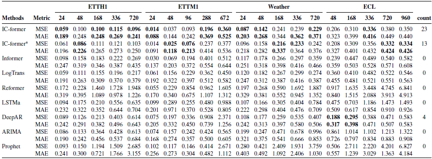
In this experiment, each model predicts time series from univariate input data. From the experimental results, we conclude the following points: IC-former gets the best results by 36. IC-former gets better results from a global perspective; Compared with Informer, the total MSE error of IC-former is reduced by 34.7%, and the total MAE error is reduced by 23.9%. Compared with Informer, the single-experiment MSE error of IC-former is reduced by at most 64.2%, and the single-experiment MAE error is reduced by at most 44.5% (at TEEH1-720).
This experiment proves that the accuracy of our proposed IC-former model in predicting a single variable is better than that of the classical sequence prediction algorithms involved in the comparison. The high accuracy provides a basis for our research on explaining neural network models.
5.2. Attention mechanism
To explore the impact of the classic attention mechanism and ProbSparse self-attention on the IC-former model, we replaced the ProbSparse self-attention in IC-former with the classic attention mechanism. IC-former* represents models with classical attention mechanisms corresponding to IC-former. It can be seen from the experimental results that although the computational cost of the classical attention mechanism is high, the accuracy improvement brought by it is relatively limited, and even most of the results are not as good as ProbSparse self-attention.
The results reflect the high efficiency of ProbSparse self-attention and prove that our proposed IC-former can effectively cooperate with various attention mechanisms, especially ProbSparse self-attention, to achieve good results.
5.3. Gait trajectory prediction
Take the data-augmented BaseData as the training set to train our proposed IC-former model. Then use GeneralizationData as the test set to test the trained model. There are four completely different gait types in GeneralizationData: stopping, going upstairs, turning around, and going downstairs. We performed tests for each of the four gaits separately.
The experimental results are shown in Fig. 4. It is worth mentioning that the four predicted gaits are not involved in the training set at all, and all of them are real data. For different gaits, the prediction accuracy of the IC-former model is satisfactory. We plotted the prediction curves for all four gait types, as shown in Fig. 5. The left curve is the input data, and the right is the predicted and real data. The prediction of the IC-former model is not only satisfactory in terms of error but also accurately predicts critical quantities as peaks and valleys of the gait trajectory for a long period.
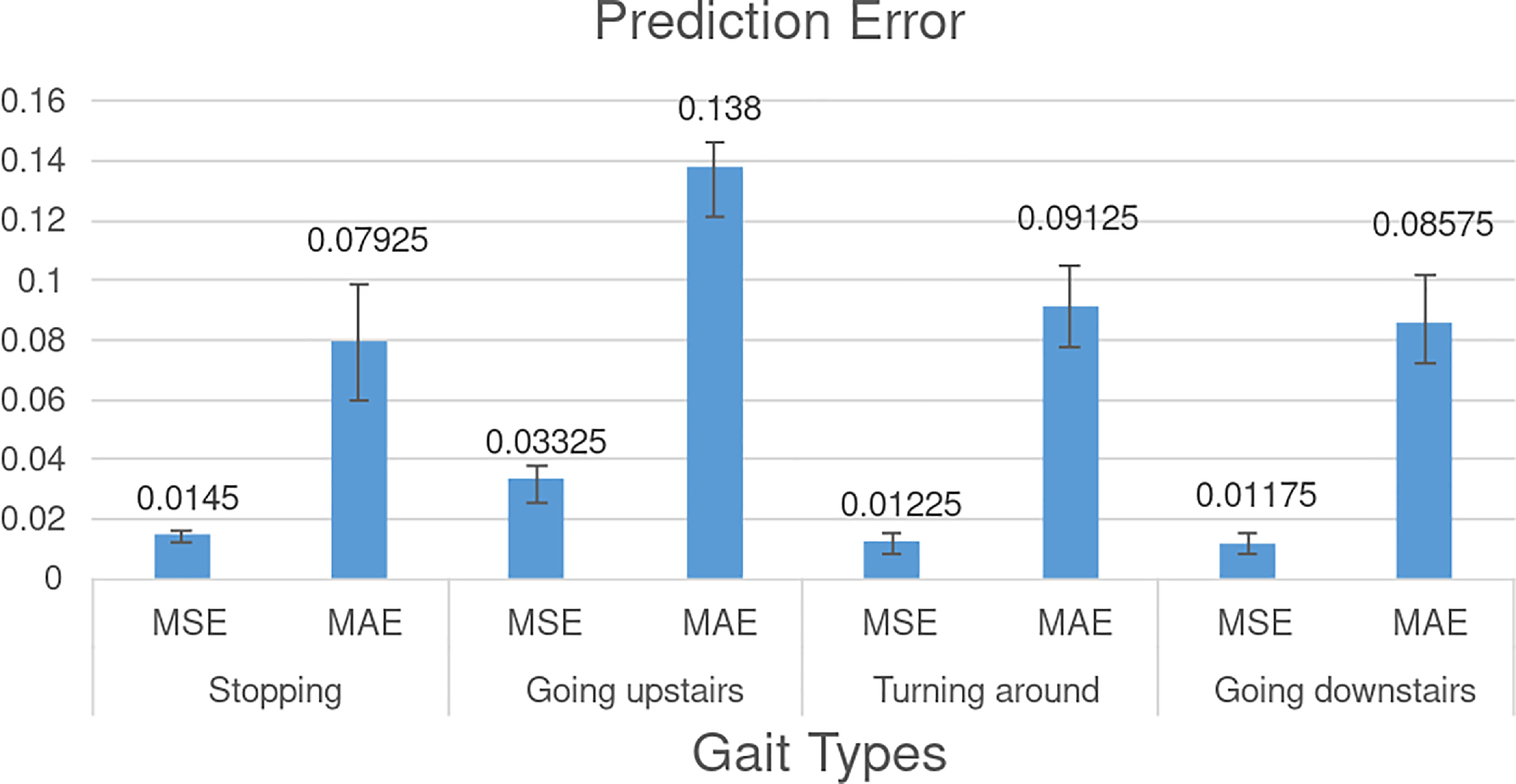
Figure 4. Gait trajectory prediction error. The value of the y-axis in the picture represents the value of the normalized gait angle.
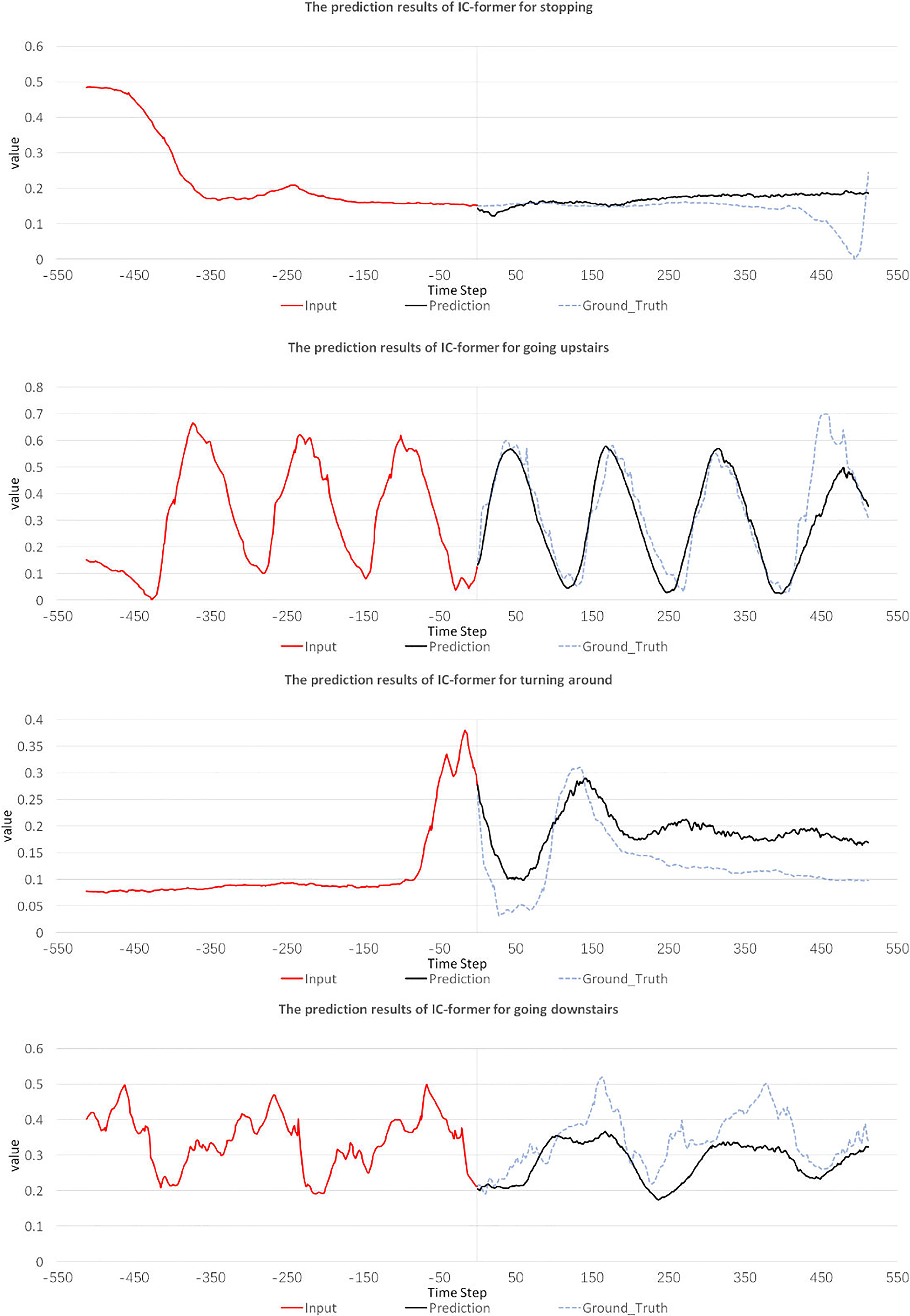
Figure 5. Predicted trajectories of the IC-former model for different gait types. The value of the y-axis in the picture represents the value of the normalized gait angle.
We trained the Informer model under the same parameters initialization method, learning rate, and other conditions as the IC-former model. The Informer model failed to predict gait trajectories in 13 randomly initialized experiments. Some prediction results of the Informer model are shown in Fig. 6. The IC-former model was trained successfully in 4 out of 13 randomly initialized experiments. The IC-former model is more accurate than the Informer model and is easier to train with stronger generalization ability.
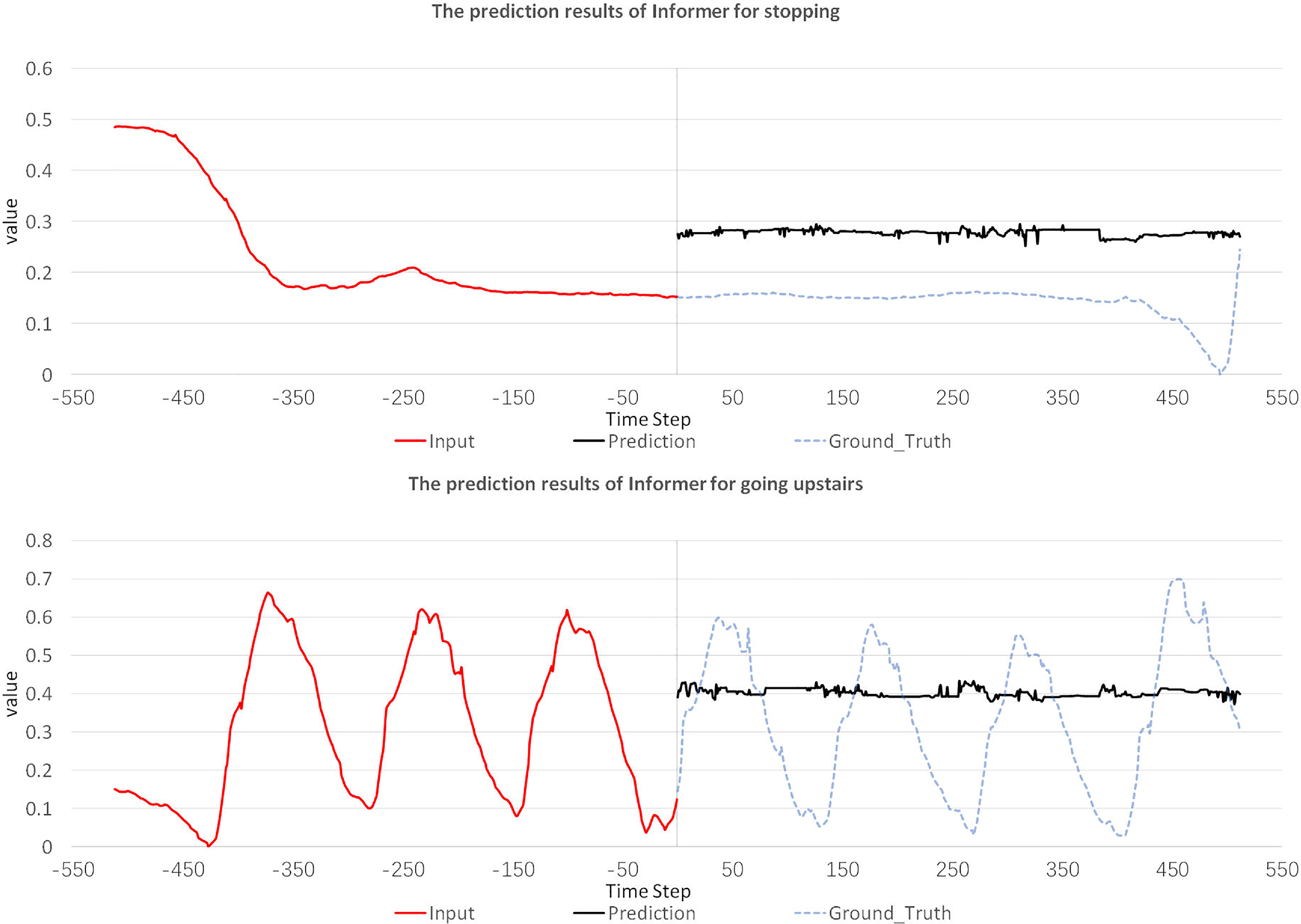
Figure 6. Predicted trajectories of the Informer model for different gait types. The value of the y-axis in the picture represents the value of the normalized gait angle.
5.4. Interpretability
In the experiment of gait trajectory prediction, the IC-former model contains a two-layer encoder and a one-layer decoder. There are three Interpretable Multi-head Attention layers. Each Interpretable Multi-head Attention layer has eight head attentions. We analyze the attention of the Interpretable Multi-head Attention layer of the IC-former model when predicting the turning gait trajectory to interpret the model.
The first is the Interpretable Multi-head Attention layer located in the first layer of the encoder. In this experiment, the encoder input of the IC-former model is a 512-length gait trajectory sequence. After a distilling layer, the data length is 256. Therefore, the size of the attention matrix of the Interpretable Multi-head Attention layer located in the first layer of the encoder is 256*256. Each number represents a segment of the original sequence of length 2.
We show the eight-head attention in Fig. 7. The distributions of the eight-head attention are quite different because different head attention extracts different features. The multi-head attention mechanism ensures the diversification of attention and feature, enhancing the robustness.

Figure 7. Head attention of the first layer of the encoder.
As shown in Fig. 8, we sum all head attention to getting total attention. When predicting the turn gait trajectory, the attention of the first layer of the encoder is focused on the end of the sequence, which is consistent with the characteristics of the turn gait trajectory.

Figure 8. The total attention of the first layer of the encoder.
We add each line of attention to get a vector of size 1*256, and the value of this vector represents the importance of the corresponding sequence segment. We draw the input–output trajectory image with the highlighted background representing the attention. From Fig. 9, we can intuitively see that attention is focused on the two peaks at the end of the trace. This shows that the two peak data contain the most abundant information for predicting trajectories.

Figure 9. Predicted trajectories of the IC-former model for turning around with the attention of the first layer of the encoder. The left curve with the heat map in the background is the input data, and the right is the output data. The higher the brightness of the heat map, the greater the weight of the corresponding input data.
The attention distribution of the second layer of the encoder is relatively uniform, and attention is concentrated on the first half of the input sequence (Fig. 10). The concentration indicates that the model extracts features from the first half of the input trajectory to fuse with features previously extracted from the second half.

Figure 10. Predicted trajectories of the IC-former model for turning around with the attention of the second layer of the encoder. The left curve with the heat map in the background is the input data, and the right is the output data. The higher the brightness of the heat map, the greater the weight of the corresponding input data.
The input to the first layer of the decoder is composed of two parts: the first part is the input gait 512-length trajectory sequence and the second part is the 512-length all-zero blank sequence. The length of the input becomes 512 through a distillation layer. The size of the attention matrix of the first layer of the decoder is 512*512. The attention distribution of the first layer of the decoder is relatively scattered, and the attention is automatically all focused on the first half with practical meaning, which is consistent with the actual nature of the input (Fig. 11).

Figure 11. Predicted trajectories of the IC-former model for turning around with attention of the first layer of the decoder. The left curve with the heat map in the background is the input data, and the right is the output data. The higher the brightness of the heat map, the greater the weight of the corresponding input data.
The above are local attention images of each layer. We splice the attention of all layers into one matrix as the global attention matrix. We plot the input–output trajectory images under global attention, as shown in Fig. 12. The attention of the second layer of the encoder is smaller than that of the other two layers, meaning the second layer obtains little information from the original input. But this does not mean that the auxiliary channel is unnecessary because, according to our experiments, the existence of the auxiliary channel does improve the model’s prediction accuracy.

Figure 12. Predicted trajectories of the IC-former model for turning around with global attention. The highlighted background representing attention is divided into three layers: from bottom to top the first layer of the encoder, the second layer of the encoder, and the first layer of the decoder.
We plot the global attention images of the same IC-former model when predicting the remaining three gaits (Figs. 13, 14, 15). Attention is mainly distributed at the input sequence’s back or front end for aperiodic gaits. For cyclic gaits, the attention is mainly distributed in the last cycle, and the peak part of the last cycle is the most important.
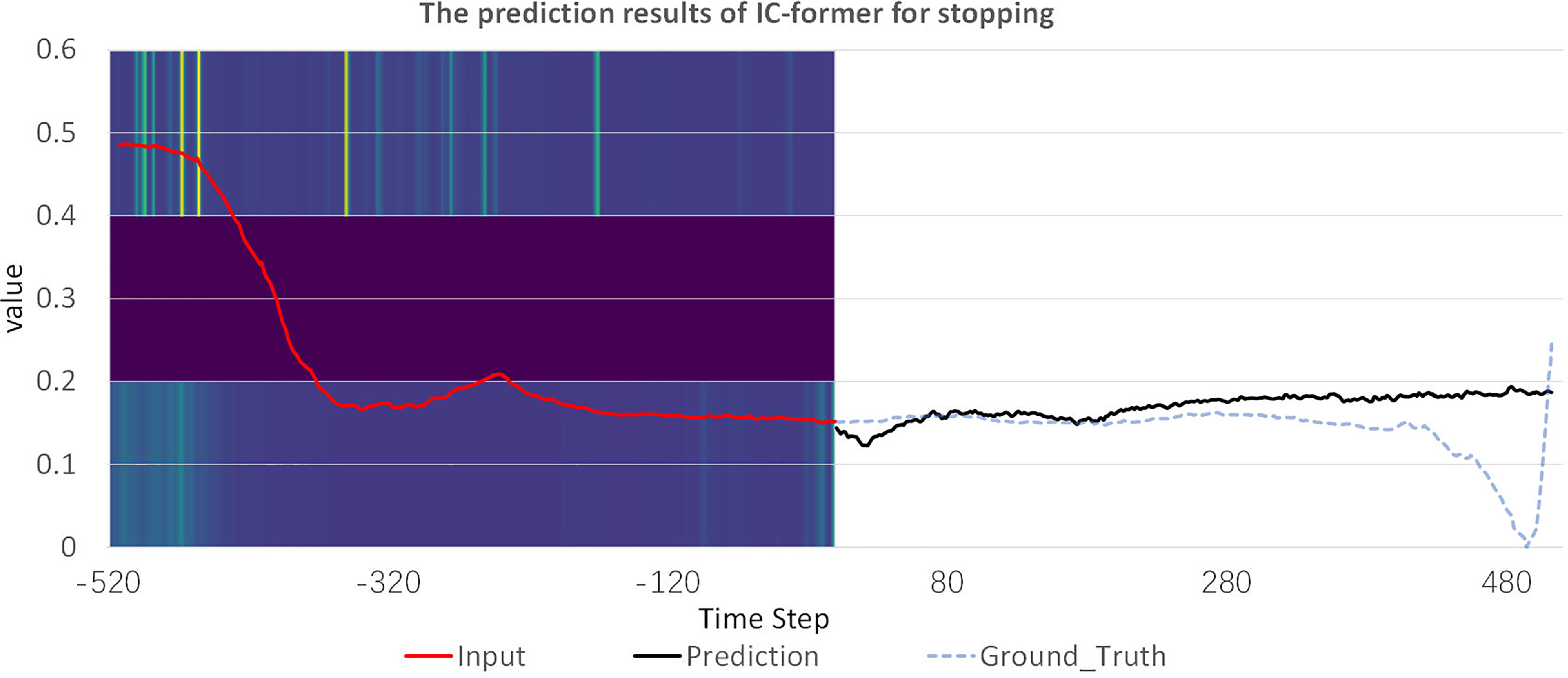
Figure 13. Predicted trajectories of the IC-former model for stopping with all attention.

Figure 14. Predicted trajectories of the IC-former model for going upstairs with all attention.

Figure 15. Predicted trajectories of the IC-former model for going downstairs with all attention.
The attention distribution of the IC-former model has two things in common when predicting different gait types.
-
1. The attention of the input sequence of the second layer of the encoder is very low, which means that the input does not provide enough features for the model.
-
2. The attention distribution of the decoder is very similar when predicting different gait types. We argue that this attention distribution is determined by the ensemble of gait data, which reflects the most informative trajectory segment overall. This attention distribution provides a good point for us to study gait data.
To further analyze and explain the IC-former for predicting gait trajectories, we plot the prediction results of another trained model for four gaits, as shown in Fig. 16.

Figure 16. Predicted trajectories of another IC-former model for going downstairs with all attention.
The attention distributions of the two models are very similar. Both set high weights for the peaks of the gait trajectory. The distribution of attention is obtained based on inherent properties, such as data and model structure, rather than randomly. The IC-former effectively reveals the data basis of the neural network model. The difference between the two attention distributions is that the former is more concentrated and plays the role of the attention mechanism better.
For public evaluation, we analyze the data interpretability of a prediction result within the ECL dataset, as shown in Fig. 17. The same as when predicting the gait trajectory, the model accurately selects the key peak data to predict the future trend of the curve.

Figure 17. Predicted trajectories of the IC-former model for ECL with attention of the first layer of the encoder.
6. Conclusion
This paper proposes the Interpretable Multi-head Attention layer and the IC-former model. The Interpretable Multi-head Attention layer preserves the input data’s mathematical meaning while enhancing the ability to extract features. The IC-former model can predict long-term sequence data with high precision and measure the input data’s importance to explain the data basis of the prediction results. We tested the IC- former model on multiple datasets. The results show that the former model exceeds the prediction accuracy of many existing sequence prediction models and successfully marks important data fragments.
Based on the IC-former model, we predict long-term gait trajectories and explain the prediction results by quantifying the importance of data at different positions in the input sequence. Important input sequence segments for predicting gait trajectories contain the richest gait information, and finding them accurately is of great significance for intent perception and gait diagnosis.
Competing interests
The authors declare no competing interests exist.
Financial support
This work was supported by the National Natural Science Foundation of China [grant numbers U21B6002].
Ethical approval
The experimental protocol is approved by the Institute Review Board of Tsinghua University (No. 20220222). All the participants gave their consent before taking part in the study.
Author contributions
Jie Yin, Ming Zhang, and Tao Zhang conceived and designed the study. Meng Chen, Chongfeng Zhang, and Tao Xue conducted data gathering. Jie Yin and Meng Chen performed statistical analyses. Jie Yin, Ming Zhang, and Tao Zhang wrote the article.


