


1. Introduction
The aim of this paper is to examine the impact of the Lagrangian mean flow, or equivalently the vorticity of the fluid, on the geometry of surface waves, their phase speed, as well as their stability properties. We find that for weakly nonlinear waves on a second-order Lagrangian mean flow, the free surface geometry does not depend on the Lagrangian mean flow to third order in the wave slope. The phase speed is modified by the Lagrangian mean flow at second order, which impacts (and can annihilate) the growth rates of the modulation instability. These results imply that instruments that use the dispersion relationship of waves, e.g. radars or optical imagery systems, measure the Lagrangian mean currents.
Currents modulate the geometry, kinematics and dynamics of deep-water surface gravity waves. The behaviour of linear inviscid waves on a shear flow has typically been examined in the Eulerian reference frame; the literature is large and spans multiple decades, e.g. Peregrine (Reference Peregrine1976), Jonsson (Reference Jonsson1990), Shrira (Reference Shrira1993), Thomas & Klopman (Reference Thomas and Klopman1997), Ellingsen & Li (Reference Ellingsen and Li2017) and numerous others. However, if the Lagrangian frame is instead used as the point of reference, the explicit role of Lagrangian drift, or equivalently the vorticity of the system, clarifies the origins of several defining characteristics of irrotational and rotational surface gravity waves.
The inverse problem – inferring information about the underlying currents from the wave field – is a central aim of remote sensing instruments. Starting with the pioneering work of Stewart & Joy (Reference Stewart and Joy1974) and continuing to this day (e.g. Smeltzer et al. Reference Smeltzer, Æsøy, Ådnøy and Ellingsen2019), researchers have tried to constrain the underlying structure of currents from measurements of the wave field. However, even in the seminal paper of Stewart & Joy (Reference Stewart and Joy1974) there is confusion about the impact of the Lagrangian mean flow on the wave phase speed. Specifically, Stewart & Joy (Reference Stewart and Joy1974) point out that a substitution of the Stokes drift as a current into their theory yields the finite amplitude Stokes correction to the phase speed. However, their theory is Eulerian and hence substituting a Lagrangian mean flow for their mean Eulerian current is inconsistent. Therefore, the correct conclusion was reached via an erroneous argument, resulting in some lingering confusion as to how the Lagrangian mean is connected to the phase speed of water waves as well as the free surface geometry. Here, we clarify these points and show, in particular, that the phase speed is affected by the Lagrangian, not the Eulerian, mean current, thus answering a long-standing question in remote sensing of currents (Chavanne Reference Chavanne2018): measured Doppler shifts of surface waves do indeed include the Stokes drift.
A formulation for permanent progressive deep-water waves on a horizontally homogeneous steady shear flow is presented. The governing equations are conservation of mass and conservation of vorticity. The conservation of mass does not specify how particles are to be labelled in a fluid, and this gauge choice (Salmon Reference Salmon2020) offers tremendous freedom in how one approaches problems in this reference frame. At the free surface we require the pressure to vanish while we assume that the waves are in deep-water and hence their induced velocity vanishes at large depths. This leads to a series of coupled equations for the coefficients of the physical locations of particles  $(a,b)$ at $(x(a,b), y(a,b))$, which are much more complicated than their Eulerian counterparts (Clamond Reference Clamond2007) as these series no longer represent analytic functions and hence cannot be related at the surface via the Hilbert transform. We derive the dynamic (pressure) boundary condition in the Lagrangian frame for permanent progressive waves which allows us to relate the Lagrangian mean flow and the phase speed of waves. Additionally, we present new general relationships between the Lagrangian mean flow and the vorticity of the waves.
As an illustration, we consider the response of the surface wave field to a weak, possibly vanishing, Lagrangian mean flow. The finite amplitude correction to the Stokes drift is shown to result in a Doppler-like shift to the frequency of these waves, which explains the curious conclusion of Stewart & Joy (Reference Stewart and Joy1974). The finite amplitude Stokes correction to phase speed sets the growth rate of the Benjamin–Feir instability (BFI) (Benjamin & Feir Reference Benjamin and Feir1967; Zakharov Reference Zakharov1968) and hence in turn there is a connection between the Lagrangian mean flow (which sets the phase speed) and the strength of this instability, as was originally noted in Abrashkin & Pelinovsky (Reference Abrashkin and Pelinovsky2017). Here, we explicitly present the growth rate of the most unstable mode and the range of unstable wavenumbers as a function of the Lagrangian mean flow.
To highlight the striking connection between the Lagrangian mean flow and the instability of finite amplitude waves, a laboratory demonstration is presented. We consider two cases, one with approximately no vertical shear (similar to Melville Reference Melville1982), and another with an imposed shear profile that nearly cancels the Stokes drift of irrotational waves. Radically different long-time behaviour is observed in the two cases. In particular, we find the BFI is largely attenuated due to the presence of the imposed shear, with wave properties closely resembling those of Gerstner more so than Stokes. Note, a full discussion of the laboratory experiments will be presented elsewhere (manuscript in preparation).
2. Governing equations
Consider inviscid deep-water surface gravity waves. The Euler equations in Lagrangian coordinates are (Lamb Reference Lamb1932; Bennett Reference Bennett2006)
 $$\begin{gather} \mathcal{J}\ddot{x}+p_ay_b-p_by_a=0, \end{gather}$$
 $$\begin{gather}\mathcal{J}\ddot{y}+p_bx_a-p_ax_b+\mathcal{J}g=0, \end{gather}$$
where  $(x,y)$ are the particle locations with the undisturbed free surface at $y=0$, $(a,b)$ are particle labels, $p$ is the kinematic fluid pressure, $g$ is the acceleration due to gravity, and $\mathcal {J}$ is defined as
 \begin{equation} \mathcal{J}=\frac{\partial(x,y)}{\partial(a,b)} \equiv x_ay_b-x_by_a = \left[ \frac{\rho(a,b)}{\rho(x,y)} \right]^{{-}1}, \end{equation}
for  $\rho$ the fluid density and subscripts denoting partial derivatives. The continuity equation may be written
 \begin{equation} u_x+v_y=\frac{\partial (\dot{x},y)}{\partial(x,y)}-\frac{\partial (\dot{y},x)}{\partial(x,y)}=\left(\frac{\partial (\dot{x},y)}{\partial(a,b)}-\frac{\partial (\dot{y},x)}{\partial(a,b)}\right)\frac{\partial(a,b)}{\partial(x,y)} =\frac{1}{\mathcal{J}}\frac{{\rm d}\mathcal{J}}{{\rm d}t}= 0, \end{equation}
where  $u=\dot {x}, v=\dot {y}$ with dots representing differentiation with respect to time. This implies
 \begin{equation} \frac{{\rm d}\mathcal{J}}{{\rm d}t}=0. \end{equation}
In order for the mapping to be invertible we also require that  $\mathcal {J}$ does not change sign.
The vorticity is defined as
 \begin{equation} \varGamma=v_x-u_y=\frac{\partial (v,y)}{\partial(x,y)}+\frac{\partial (u,x)}{\partial(x,y)}=\frac{1}{\mathcal{J}}\left(\dot{x}_ax_b-\dot{x}_bx_a+\dot{y}_ay_b-\dot{y}_by_a\right). \end{equation}
Equations (2.1) and (2.2) imply that vorticity is conserved, that is  $\dot {\varGamma }=0$. For irrotational flows $\varGamma =0$. Furthermore, through this discussion we assume $\varGamma \to 0$ as $b\to -\infty$.
The pressure  $p$ must vanish at the free surface, which we choose to occur at $b=0$ so that $p=0$ at $b=0$. Finally, we take the bottom to be the limit as $b\to -\infty$, so that $\dot {y}\to 0$ at $b\to -\infty$.
2.1. Series expansions
We consider permanent progressive monochromatic waves progressing with velocity  $c$, so that we assume the map between $(x,y)$ and $(a,b)$ takes the form
 \begin{equation} x=a+U(b)t +\sum_{n=1}^{\infty} x_n(b) \sin \theta_n; \quad y=b+y_0(b) +\sum_{n=1}^{\infty} y_n(b) \cos \theta_n, \end{equation}
where  $\theta _n = nk(a-(c-U(b))t)$, $k$ is the wavenumber and $U$ is the Lagrangian mean flow. We are considering the intrinsic frequency here, as this eliminates secular terms (Buldakov, Taylor & Taylor Reference Buldakov, Taylor and Taylor2006; Clamond Reference Clamond2007). There is some question as to the convergence of these Lagrangian expansions, which have been formally studied for Gerstner waves (Henry Reference Henry2008; Constantin Reference Constantin2011). This is discussed in Clamond (Reference Clamond2007), where it is shown numerically that there is series convergence even for the highest wave, although the convergence rates are slow. A full discussion of this point is outside of the scope of this manuscript, but here we assume that the expansions given by (2.7a,b) converge. Note, Clamond (Reference Clamond2007) assumed that $k=k(b)$ while here we take $k$ as a constant. This changes the values of wave amplitude that give particular values of $ak$, but all physical quantities remain the same.
The mean surface level,  $y_0(0)\equiv \langle y \rangle |_{b=0}$ (here $\langle \dots \rangle =(2{\rm \pi} / k)^{-1}\int _0^{2{\rm \pi} / k}(\dots )\,\mathrm {d}a$ is phase averaging), is found by inserting (2.7a,b) into (2.3) and phase averaging to find
 \begin{equation} y_0(b)={-}\frac{1}{2}\sum k n x_n y_n+\int_{-\infty}^b (\langle \mathcal{J}\rangle-1) \,\mathrm{d} \beta+y_0^0, \end{equation}
where  $y^0_0$ is a constant of integration that is determined by the proper choice of the Bernoulli head, ensuring that $\langle yx_a|_{b=0} \rangle = 0.$ Note, it is understood here and henceforth that an integration variable $\beta$ replaces $b$ in the integrands, and $\sum$ implies summing $n$ from $1$ to $\infty$.
The Lagrangian drift arises as a kinematic constraint that requires the vorticity to be time independent, so that from the mean component of the vorticity we find
 \begin{equation} U = \frac{\dfrac{c}{2}\displaystyle\sum n^2k^2 (x_n^2+y_n^2)-\gamma}{1+\dfrac{1}{2}\displaystyle\sum n^2k^2(x_n^2+y_n^2)}, \end{equation}
where  $\gamma \equiv \langle \int _{-\infty }^{b} \varGamma \mathcal {J} \,\mathrm {d} \beta \rangle$. This equation implies that if the vertical behaviour is simple in $(x_n,y_n)$, e.g. of exponential decay form, it will not be simple in $U$, and vice versa.
From (2.9) we also see that the vorticity and Lagrangian mean flow are intimately related. If we prescribe the vorticity, this then constrains the form of the drift, and vice versa. This will be made clearer in the asymptotic example considered below.
2.2. Free surface pressure condition
Next, we can find other relationships between  $y_0$, $U$ and $c$ by solving for the pressure. That is, multiplying (2.1) by $x_b$ and (2.2) by $y_b$, we find
 \begin{equation} p_b+gy_b+\ddot{y}y_b+\ddot{x}x_b=0. \end{equation}
Next, by differentiating the series expansions for  $(x,y)$ we find $\ddot {y}=-(c-U)\dot {y}_a,$ and $\ddot {x}=-(c-U)\dot {x}_a$ so that
 \begin{equation} p_b+gy_b-(c-U)\left(\dot{y}_ay_b+\dot{x}_ax_b\right)=0. \end{equation}
We can rewrite the expression in the final parentheses using the definition of the vorticity, (2.6), to find
 \begin{equation} p_b+gy_b-(c-U)\left(\varGamma\mathcal{J}+\dot{x}_bx_a+\dot{y}_by_a\right)=0. \end{equation}
We can relate space and time derivatives via  $x_a = 1+((U-\dot{x})/(c-U))$ and $y_a=-\dot {y}/(c-U),$ so that (2.12) may be written as
 $$\begin{gather} \left[p+gy+\tfrac{1}{2} (\dot{x}-c)^2+\tfrac{1}{2} \dot{y}^2\right]_b -(c-U)\mathcal{J}\varGamma =0 \end{gather}$$
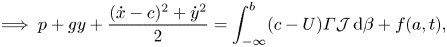 $$\begin{gather}\implies p+gy+\frac{(\dot{x}-c)^2+\dot{y}^2}{2}=\int_{-\infty}^b (c-U)\varGamma\mathcal{J} \,\mathrm{d} \beta +f(a,t), \end{gather}$$
where  $f(a,t)$ is a constant of integration which must be ${c^2}/{2}$ so that $\langle p(b=0)\rangle =0$. When $\varGamma =0$ we return a recognizable form of Bernoulli's equation for irrotational permanent progressive waves.
The dynamic boundary condition requires  $\langle p\rangle$ = 0 at $b=0$, so that we can find an expression for the phase velocity in terms of $y_0$ and $U$ at the surface (note the constant of integration for $y_0$ must be correct to employ this – e.g. for Gerstner waves $y^0_0$ is not zero and is given explicitly in the next section), which yields
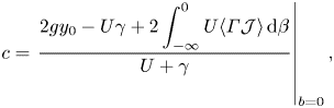 \begin{equation} c=\left.\frac{2gy_0-U\gamma+2\displaystyle\int\nolimits^0_{-\infty} U\langle \varGamma\mathcal{J}\rangle \,\mathrm{d} \beta}{U+\gamma}\right|_{b=0}, \end{equation}
where we have used the fact that  $\langle \dot {x}^2+\dot {y}^2 \rangle = U^2+(c-U)^2\sum n^2k^2(x_n^2+y_n^2)/2=c(\gamma +U)-U\gamma$, which is found by solving for $\sum k^2n^2(x_n^2+y_n^2)$ in (2.9). Equation (2.15) reduces in limiting scenarios. First, when $\varGamma =0$, $c={2gy_0}/{U}|_{b=0},$ while for $U= 0$ we have $c={2gy_0}/{\gamma }|_{b=0}.$
Notice in (2.15) that  $c$ is determined by the Lagrangian, not Eulerian, current. Even with zero Eulerian current, $c$ obtains a Doppler-like shift due to Stokes drift. We can then answer the question of Chavanne (Reference Chavanne2018): the observed Doppler shift of waves do indeed include the Stokes drift as well as the Eulerian current.
In the classical approach to examining Stokes waves in an Eulerian framework, the condition that  $p=0$ at the free surface, together with the analyticity of the velocity potential and stream function, is enough to reduce the problem to a boundary value system which may be solved algebraically (Schwartz Reference Schwartz1974; Balk Reference Balk1996). In the Lagrangian frame it is clear that the velocity potential and stream function do not satisfy the Cauchy–Riemann equations and hence are not analytic. In general, the series expansions for $z = x+\mathrm {i} y$ depend on both $s=a+\mathrm {i} b$ and $\bar {s} = a-\mathrm {i} b$. A simple example is given by Gerstner's wave, which takes the form $kz = ks + \mathrm {i} \epsilon \exp ({\mathrm {i} k\bar {s} -\mathrm {i}k ct})$ for $\epsilon$ a wave slope and $c$ a phase velocity (Lamb Reference Lamb1932, § 251). We see immediately that $z_{\bar {s}}\neq 0$ and hence $z$ is not analytic. A more general approach is then needed to examine solutions to this system of equations. This will be pursued elsewhere and instead for the rest of the present study we illustrate the physical implications of the Lagrangian drift by considering asymptotic solutions in limiting cases.
3. Weakly nonlinear waves on a weak shear flow
As our starting point we take Gerstner's (Lamb Reference Lamb1932, § 251) remarkable, exact surface wave solution
 \begin{equation} kx = ka -\epsilon \sin (k(a-c t)) e^{k b}; \quad ky = \tfrac{1}{2}\epsilon^2 + kb +\epsilon \cos (k(a-c t))e^{kb}, \end{equation}
where  $\epsilon$ is the wave slope. These waves have no mean Lagrangian transport – their particle trajectories are circles. Since $U(b)=0$, (2.15) implies $c=\sqrt {g/k}$, independent of $\epsilon$. As discussed in Clamond (Reference Clamond2007), the mean water level is $k^{-1}\epsilon ^2/2$; although not usually written explicitly, this term is crucial to properly compute $c$. Note, Gerstner waves are finite amplitude exact solutions which possess interesting stability properties of their own (Leblanc Reference Leblanc2004; Ionescu-Kruse Reference Ionescu-Kruse2018).
The determinant of the Jacobian of the mapping from physical space to label space is  $\mathcal {J} = 1 -\epsilon ^2 e^{2kb}$ while the vorticity may be found through the relation $\varGamma \mathcal {J} = 2ck\epsilon ^2 e^{2kb}$.
To transform these Lagrangian solutions to the Eulerian frame we must find  $a=a(x)$. This inversion is not possible in closed form, as it essentially reduces to solving Kepler's equation and so we must invert this relationship iteratively at each order of $\epsilon$.
Defining  $\eta$ as $\eta = y(a(x),b=0,t)= y(x,t),$ then to $O(\epsilon ^3),$ where $\epsilon \ll 1$, we find
 \begin{equation} ka = kx+\epsilon \sin \theta_0 +\frac{\epsilon^2 }{2}\sin 2\theta_0 -\frac{\epsilon^3}{8} \left(\sin\theta_0-3\sin 3\theta_0\right), \end{equation}
at  $b=0$ so that
 \begin{equation} k\eta = \left(\epsilon - \frac{3\epsilon^3}{8}\right) \cos \theta_0 +\frac{\epsilon^2}{2}\cos 2\theta_0 +\frac{3\epsilon^3}{8} \cos 3\theta_0+\dots, \end{equation}
where  $\theta _0 = k(x-c_0t)$ and $c_0 = \sqrt {g/k}.$ Note, there is a second-order correction to the mean surface level in the Lagrangian frame, but there is no correction to $O(\epsilon ^3)$ in the Eulerian frame (Longuet-Higgins Reference Longuet-Higgins1986).
We can also find the horizontal and vertical Eulerian velocities  $(u,v)$ to $O(\epsilon ^3)$. This involves finding $a=a(x,y)$ and $b=b(x,y)$ to third order, which gives
 $$\begin{gather} k a(x,y) = kx+\left(\epsilon+\frac{\epsilon^3}{2}(1-e^{2ky})\right) \sin\theta_0 e^{ky}, \end{gather}$$
 $$\begin{gather}kb(x,y) = ky-\left(\epsilon +\frac{\epsilon^3}{2}({-}1+3e^{2ky}) \right)\cos \theta_0 e^{ky} +\epsilon^2\left(-\frac{1}{2}+e^{2ky}\right) . \end{gather}$$
 Inserting these into (3.1a,b), the Eulerian velocity fields  $(u,v)=(\dot {x},\dot {y})$ are given by
 $$\begin{gather} u(x,y,t) = c_0 \left(\epsilon+\frac{\epsilon^3}{2}\left({-}1+3e^{2ky}\right)\right) \cos \theta_0 e^{ky} - c\epsilon^2 e^{2ky}; \end{gather}$$
 $$\begin{gather}v(x,y,t) = c_0 \left(\epsilon -\frac{\epsilon^3}{2}\left(1-e^{2ky}\right)\right) \sin \theta_0e^{ky}, \end{gather}$$
so that we see that Gerstner waves require there to be a non-zero horizontal Eulerian mean flow at second order that is equal and opposite to the Stokes drift.
3.1. Third-order weakly rotational and irrotational waves
Next we find the third-order expansions for Stokes waves by expanding the Gerstner waves solutions to include  $O(\epsilon ^2)$ Lagrangian mean flows, $\epsilon ^2 U(b)$ (see also the related discussions in Abrashkin & Pelinovsky Reference Abrashkin and Pelinovsky2017, Reference Abrashkin and Pelinovsky2018). Going through the algebra, we find
 \begin{gather} kx = ka + kU(b)t - \left(\epsilon e^{kb}+\frac{\epsilon^3}{k} F'(b)\right)\sin \theta_L; \quad ky = kb + \frac{1}{2}\epsilon^2 +\left(\epsilon e^b +\epsilon^3 F(b)\right)\cos \theta_L, \end{gather}
where  $\theta _L = k(a-(c- \epsilon ^2 U)t)$ and $F \equiv ({2k}/{c})e^{-kb}\int _{-\infty }^b e^{2k\beta } U(\beta ) \,\mathrm {d} \beta.$ Note, the phase now has dependence on $b$ and $c$ is unknown at this stage.
The mean water level  $y_0$ is $O(\epsilon ^2)$ in the Lagrangian reference frame, compared with $O(\epsilon ^3)$ in the Eulerian frame (Longuet-Higgins Reference Longuet-Higgins1986).
Insertion into (2.3) and (2.6) gives Jacobian  $\mathcal {J} = 1-\epsilon ^2 e^{2kb},$ and vorticity
 \begin{equation} \varGamma = \epsilon^2(2kce^{2kb}-U'(b)). \end{equation}
When  $U=c e^{2kb}$, the flow is thus irrotational and we return the well-known expansions for Stokes waves to third order in $\epsilon$.
Equation (3.9) is of central importance – it relates the vorticity of the system to gradients of the Lagrangian mean flow. At this order, the right-hand side of (3.9) is the curl operator, so we return a main result from generalized Lagrangian mean theory (Bühler Reference Bühler2014), namely that the vorticity of the system is given by the difference of the curl of the pseudomomentum and the Lagrangian mean flow. A similar equation arises when one allows for finite bandwidth effects and offers a clear motivation for the long wave response, or Bretherton flow, of a wave packet (Salmon Reference Salmon2020; Pizzo & Salmon Reference Pizzo and Salmon2021).
Additionally, the phase velocity  $c$ is found to be
 \begin{equation} c = c_0 \left(1+\epsilon^2 F(0)\right) = c_0 \left(1 + \epsilon^2 \left(\frac{2k}{c_0}\int_{-\infty}^0 e^{2k\beta}U(\beta) \,\mathrm{d} \beta\right)\right). \end{equation}
When  $U=0$, we return the expansions for the Gerstner wave while for an irrotational wave, $U=c_0 e^{2kb}$ and we return the phase velocity with the Stokes correction, i.e. $\frac {1}{2}\epsilon ^2$. Note, unlike Stewart & Joy (Reference Stewart and Joy1974), we have used a consistent argument to return this result.
Inversion methods for inferring the underlying currents from the wave field rely on measuring deviations of the wave phase velocity from that in quiescent waters. The phase velocity deviation in (3.10) implies that such inversion methods are sensitive to the Lagrangian mean flow. A comprehensive analysis would involve considering a broadband wave spectrum with contributions to the Stokes drift from many wavenumbers, which is outside the scope of the present work.
As we did for the Gerstner wave in (3.3), we can map (3.8a,b), under the constraint that the flow is irrotational, to the Eulerian frame, finding
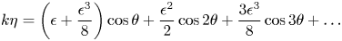 \begin{equation} k\eta = \left(\epsilon + \frac{\epsilon^3}{8}\right) \cos \theta +\frac{\epsilon^2}{2} \cos 2\theta +\frac{3\epsilon^3}{8} \cos 3\theta+\dots\end{equation}
where  $\theta = k(x-ct)$ and $c= c_0 (1+\frac {1}{2}\epsilon ^2)$ follows from (3.10).
When comparing (3.11) and (3.3), we see immediately that the second harmonic of  $\eta$ is the same for Gerstner and Stokes waves, and hence is not related to the Lagrangian mean flow. If we define a new small parameter $\mu = \epsilon -(\epsilon^3/2)$ then $k\eta = (\mu-(3\mu^3/8))\cos \theta +(\mu^2/2)\cos2\theta +(3\mu^3/8)\cos 3\theta$, which implies that Stokes waves and Gerstner waves have identical free surface geometries to third order (Clamond Reference Clamond2007).
Additionally, we can find the velocity in the Eulerian frame. Again, we need to write down the depth-dependent mappings:
 $$\begin{gather} ka(x,y) = kx-c_0k\epsilon^2 t e^{2ky}+\left(\epsilon +\frac{\epsilon^3}{2}\left({-}1+4e^{2ky}\right) \right) \sin \theta e^{ky}+2\epsilon^3 c_0 k t \cos \theta e^{3ky}, \end{gather}$$
 $$\begin{gather}kb(x,y) = ky+\epsilon^2\left(-\frac{1}{2}+e^{2ky}\right)-\left(\epsilon+\frac{\epsilon^3}{2}\left({-}1+4e^{2ky}\right) \right) \cos\theta e^{ky}. \end{gather}$$
Substituting these relationships into the velocity field for this case of irrotational flow, we find
 \begin{equation} u = \epsilon c \cos\theta e^{ky}; \quad v = \epsilon c \sin\theta e^{k y}, \end{equation}
which agrees with the classical result for third-order Stokes waves.
Although not considered here, one may also examine mixed Eulerian–Lagrangian maps in the spirit of Virasoro (Reference Virasoro1981). This may have applications to the interpretation of current measurements from uncrewed mobile platforms like the Liquid Robotics Wave Glider (Grare et al. Reference Grare, Statom, Pizzo and Lenain2021).
3.2. Modulation instability
The form of the phase velocity is enough to provide a heuristic derivation of the nonlinear Schrödinger equation (NLSE) on a weak Lagrangian shear flow (Abrashkin & Pelinovsky Reference Abrashkin and Pelinovsky2017), following the classical geometrical optics approach (Benjamin & Feir Reference Benjamin and Feir1967; Yuen & Lake Reference Yuen and Lake1982; Abrashkin & Pelinovsky Reference Abrashkin and Pelinovsky2018). Whereas previous, Eulerian derivations of the NLSE in the presence of shear have favoured the special case of constant vorticity which permits potential theory (Baumstein Reference Baumstein1998; Thomas, Kharif & Manna Reference Thomas, Kharif and Manna2012); the Lagrangian framework handles arbitrary  $U(b)$ more readily.
Here, we take  $\epsilon = \epsilon _0 A$ for some complex valued dimensionless amplitude $A$ of ${O}(1)$, and we drop the subscript on $\epsilon$ for clarity of presentation. We regard the reference system where the constant of integration for U in (3.9) is zero, and define
 \begin{equation} \mathcal{V} \equiv 2\frac{k}{c}\epsilon^2 \int_{-\infty}^0e^{2k\beta} U(\beta) \,\mathrm{d} \beta, \end{equation}
which implies the dispersion relationship is given by  $\omega = \omega _0 (1+ \mathcal {V})$ with $\omega _0=k_0c_0=\sqrt {gk_0}$ with $k_0$ the wavenumber of the unmodulated regular wave.
Following Abrashkin & Pelinovsky (Reference Abrashkin and Pelinovsky2018), we take a geometrical optics approach and let  $\omega = \omega _0+ \mathrm {i} \epsilon \partial _t$ and $k = k_0 -\mathrm {i}\epsilon \partial _x ,$ where we have expanded about a carrier wave with frequency $\omega _0$ and wavenumber $k_0$. Multiplying the dispersion relationship by $A$, we find that to $O(\epsilon ^3)$
 \begin{equation} \mathrm{i} A_{\tau}- {\tfrac{1}{8}} A_{\chi \chi}-2A\mathcal{V} = 0, \end{equation}
where  $\tau = \epsilon ^2 \omega _0 t$ and $\chi =\epsilon k_0(x-c_{g0} t )$ where the group velocity is $c_{g0}={\textstyle \frac 12} c_0$ .
A solution to this NLSE, (3.16), is  $A=a_0 \exp ({-2\mathrm {i}\mathcal {V}\tau })$, and we define $k_0K$ and $\omega _0\varOmega$ as the wavenumber and frequency of a perturbation to this solution, respectively. Taking a perturbation of this solution of the form $A= (a_0+\delta _+\exp ({\mathrm {i} (\varOmega \tau +K\chi )})+\delta _-\exp ({\mathrm {i} (\varOmega \tau - K\chi )}))\exp ({-2\mathrm {i} \mathcal {V}\tau })$, we find that to lowest order in $(\delta _+,\delta _- )$ the system obeys
 \begin{equation} \begin{pmatrix}
2\mathcal{V}-(K^2/8)-\varOmega & 2\mathcal{V}\\ 2\mathcal{V}
& 2\mathcal{V}-(K^2/8)+\varOmega \end{pmatrix}
\begin{pmatrix} \delta_+\\ \delta_- \end{pmatrix} =
\begin{pmatrix} 0 \\ 0 \end{pmatrix}.
\end{equation}
\begin{equation} \begin{pmatrix}
2\mathcal{V}-(K^2/8)-\varOmega & 2\mathcal{V}\\ 2\mathcal{V}
& 2\mathcal{V}-(K^2/8)+\varOmega \end{pmatrix}
\begin{pmatrix} \delta_+\\ \delta_- \end{pmatrix} =
\begin{pmatrix} 0 \\ 0 \end{pmatrix}.
\end{equation}
Non-trivial solutions exist when the determinant of the matrix is zero, which implies  $\varOmega ^2 = \frac {1}{8}((K^2/8)-4\mathcal{V})K^2$.
The system is unstable when  $\mathcal {V}>0$ and
 \begin{equation} 0< K<4\sqrt{2\mathcal{V}}, \end{equation}
while the most unstable wavenumber occurs when  $K=4\sqrt {\mathcal {V}}$ with growth rate
 \begin{equation} |\varOmega_{max}| = 2 \mathcal{V}. \end{equation}
The relations (3.18) and (3.19), although implicit in Abrashkin & Pelinovsky (Reference Abrashkin and Pelinovsky2018), were not presented there. We see that the growth rate of the instability may be strongly modified (i.e. it is zero for Gerstner waves) and the range of wavenumbers that are unstable can vary considerably as a function of the drift.
We now discuss a laboratory demonstration of this deep result.
4. Laboratory demonstration of the impact of the Lagrangian mean flow on the Benjamin–Feir instability
The laboratory demonstration discussed below was conducted in the recirculating water channel at Norwegian University of Science and Technology. See Jooss et al. (Reference Jooss, Li, Bracchi and Hearst2021) for further details. The test section is  $11.2$ m long, $1.8$ m wide and is outfitted with a plunger wave maker at the outlet, generating waves propagating upstream on the flow. At the inlet the incoming flow of depth $0.5$ m is controlled by an active grid which allows us to tailor the vertical shear. The active grid consists of horizontal and vertical bars spaced by $10$ cm with square wings attached, each wing measuring $10$ cm along the diagonal. Each bar is controlled by a stepper motor. The five submerged horizontal grid bars were actuated in a flapping motion relative to the position of least flow blockage. We use the flapping to design two flow profiles. For an approximately depth-uniform mean flow, all bars were flapped through an angle of ${\pm }45^\circ$. A second profile with near-surface vertical shear approximately cancelling the Stokes drift profile was created by keeping the shallowest bar fixed in a position of least blockage while the deeper bars were flapped through an angle of ${\pm }60^\circ$. The vertical grid bars were always fixed in the position of least blockage. In the centre of the channel eight wave gauges, at locations $\{1.703, 1.914, 3.719, 3.924, 5.722, 5.929, 7.719, 7.928\}$ metres from the wave maker measured the free surface displacement. Laser Doppler velocimetry ( $60$ mm FiberFlow probe, Dantec Dynamics) was used to measure the near-surface current profiles.
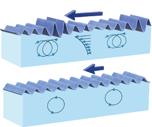
Figure 1 illustrates how the Lagrangian mean flow can alter the BFI growth rates. In particular, when the induced flow has negligible shear, as plotted in figure 1(a), we see the strong groupiness in the wave field, signifying the flux of energy from the finite amplitude carrier waves to the sidebands, which is clear from the spectral plot shown in figure 1(c). The waves have slope  $0.17$ (–) and wavenumber $6.0\ ({\rm rad}\ {\rm m}^{-1})$. Strikingly, when an Eulerian mean shear current is generated that approximately cancels the Stokes drift (such that the Lagrangian drift $U\approx 0$), the BFI is strongly suppressed. This is evident by the time series, which shows only weak modulations of the wave amplitude. Correspondingly, we find a far weaker sideband and low-frequency response. The sideband growth is strongly asymmetric, which is not accounted for in the theory. However, the higher frequency sideband is much closer to the carrier wave frequency than in the case of minimal shear, in agreement with (3.18). Note, the waves in figure 1(b) more closely resemble those of Gerstner than those of Stokes. This discussion is meant to serve as a demonstration of the ideas presented in this manuscript, particularly in § 3.2. The BFI weakening from constant mean shear was observed by (Steer et al. (Reference Steer, Borthwick, Stagonas, Buldakov and van den Bremer2020), see also Simmen & Saffman Reference Simmen and Saffman1985; Baumstein Reference Baumstein1998; Thomas et al. Reference Thomas, Kharif and Manna2012); a tailored profile based on the Lagrangian theory enabled this arguably even more striking demonstration. A detailed quantitative analysis, beyond the scope of this manuscript, is currently in preparation.

Figure 1. The evolution of finite amplitude surface gravity waves in a wave channel with two imposed shear currents – one that is approximately uniform (a,b) and one whose shear acts to approximately cancel the Stokes drift so that the Lagrangian current  $U\approx 0$ (c,d). Steepness and wavenumbers are (a) $0.176$ and $6.01\ ({\rm rad}\ {\rm m}^{-1})$ and (c) $0.174$ and $6.06\ ({\rm rad}\ {\rm m}^{-1})$. Eulerian (Lagrangian) currents are shown with solid (dashed) lines in (b,d) and wave spectra in (e).
5. Conclusions
In this paper we have presented a novel formulation for permanent progressive waves on a horizontally uniform time-independent Lagrangian mean. We related fundamental properties of the waves, viz. their vorticity and phase velocity, with the Lagrangian mean flow. We then presented the explicit connection between the Lagrangian mean flow and wave geometry, kinematics and dynamics for the scenario when the Lagrangian mean flow was weak. This included explicit expressions for the dependence of the Benjamin–Feir instability growth rate (Abrashkin & Pelinovsky Reference Abrashkin and Pelinovsky2017, Reference Abrashkin and Pelinovsky2018), as well as the range of unstable perturbation wavenumbers and frequencies, on the Lagrangian mean flow. To illustrate these points, we presented results from a recent laboratory demonstration that highlight the striking dependence of finite amplitude wave behaviour on the underlying shear flow.
Our theoretical results imply that the nonlinear source term in the wave action evolution equation (Hasselmann Reference Hasselmann1973; Phillips Reference Phillips1985) should have growth rates that depend on the shear in the underlying flow. In particular, (3.19) shows how the growth rate depends on both the wave slope and the underlying Lagrangian mean flow. If there are external currents, then this can potentially modify the instability growth rates and hence the wave action flux (Longuet-Higgins Reference Longuet-Higgins1976). As the upper ocean is sheared, a better understanding of the implications of this work for weak wave turbulence are of particular interest and of significant potential impact to the wave modelling community.
Finally, our results can be used to infer information about sub-surface currents based on observations of the surface wave field. We emphasize that it is the Lagrangian, not the Eulerian, current which can be measured remotely from wave dispersion alone. Specifically, the explicit mappings between Lagrangian and Eulerian reference frames for the Stokes and Gerstner waves highlight that the Lagrangian mean does not modulate free surface geometry to third order. Instead the higher order corrections arise due to the nonlinear mapping between the frames. However, the Lagrangian mean flow does show up as a Doppler-like shift to the wave frequency. A comprehensive discussion of a set of laboratory experiments on wave geometry, kinematics and dynamics for waves on a shear flow is in preparation.
Acknowledgements
N.P. thanks R. Salmon for many useful discussions on these topics, which directly motivated the present investigation.
Funding
N.P. and L.L. were partially supported by NSF grant OCE-2219752 and NASA grant 80NSSC19K1688. S.Å.E. was supported by Research Council of Norway grant 325114.
Declaration of interests
The authors report no conflict of interest.


 Open access