2 Data and notation

Following the notation in Wahl et al. (Reference Wahl, Lindholm and Verrall2019), let $N_{ij}$ denote the number of claims that occurred in accident year i, $i=1,...,m$ and were reported j, $j=1,\ldots, d$ years after occurring, and let $X_{ijk}$ denote the sum of all incremental payments from claims that incurred in year i, were reported j years after that and paid k, $k=1,...,\kappa$ years after being reported, where $\kappa$ is the maximum payment delay. While it is possible to use different maximum delays for reporting claims and payments, respectively, only $d=\kappa=m-1$ will be considered in this paper. For more on this, see, for example, Verrall et al. (Reference Verrall, Nielsen and Jessen2010), Wahl et al. (Reference Wahl, Lindholm and Verrall2019).

Further, let $N^{\textrm{open}}_{ijk}$ denote the number of claims that incurred in accident year i, were reported j years thereafter that are open at the end of the k:th year thereafter, that is open at the end of year $i + j + k$ . Thus, $N^{\textrm{open}}_{ijk} \leq N_{ij}$ for all $k=0,...,m-1$ . Let $N^{\textrm{stay-open}}_{ijk}$ and $N^{\textrm{re-open}}_{ijk}$ denote the number of open claims that were and were not open in the previous year, respectively. Note that

\begin{equation*}N^{\textrm{open}}_{ijk} =N^{\textrm{re-open}}_{ijk}+N^{\textrm{stay-open}}_{ijk}.\end{equation*}

Consider a setting where one has access to data from the perspective of the first day of the $m+1$ :th year. That means that all data $N_{ij}$ such that $i+j \leq m$ and all data $X_{ijk}$ , $N^{\textrm{open}}_{ijk}$ , $N^{\textrm{re-open}}_{ijk}$ , $N^{\textrm{stay-open}}_{ijk}$ such that $i+j+k \leq m$ is available, which can be formalised using the index set

\begin{equation*}\mathcal{A}_0 = \left\{(i, j, k):\, i + j + k \le m \right\},\end{equation*}

as the data sets

\begin{align*}\mathcal{X}_0 &= \left\{X_{ijk} :\, (i,j,k) \in \mathcal{A}_0 \right\},\\[3pt] \mathcal{N}^{+}_0 &= \left\{N_{ij},N^{\textrm{re-open}}_{ijk},N^{\textrm{stay-open}}_{ijk} :\,(i,j,k) \in \mathcal{A}_0 \right\}.\end{align*}

In certain cases, we might not have access to how many of the open claims stem from re-openings or not, and in those cases $\mathcal{N}_0^+$ will have to be replaced by the less granular set

\begin{equation*}\mathcal{N}_0 = \left\{N_{ij},N^{\textrm{open}}_{ijk} :\,(i,j,k) \in \mathcal{A}_0 \right\}.\end{equation*}

3 Explicit modelling of closings and re-openings of claims – the CRMO model

The aim of the current paper is to introduce an extension of the CRM that was introduced in Wahl et al. (Reference Wahl, Lindholm and Verrall2019), which allows for closing and re-opening of claims, including multiple re-openings and closings per claim. This new model will be abbreviated CRMO, where “O” stands for “openness dynamics”.

Following Wahl et al. (Reference Wahl, Lindholm and Verrall2019), we let $N_{ij}$ follow an over-dispersed Poisson distribution with intensity parameter $\nu_{ij}$ and over-dispersion parameter $\phi$ , that is

(3.1) \begin{equation}\begin{split}\mathbb{E}\left[ N_{ij}\right] & = \nu_{ij}, \\[3pt] \textrm{Var}\left(N_{ij}\right)& = \phi\mathbb{E}\left[ N_{ij}\right].\end{split}\end{equation}

Further, note that $N^{\textrm{open}}_{ijk}$ can be expressed as a sum of boolean variables,

\begin{equation*} N^{\textrm{open}}_{ijk} = \sum \limits_{l=1}^{N_{ij}} N^{\textrm{open}}_{ijkl},\end{equation*}

where $N^{\textrm{open}}_{ijkl}=1$ if claim l of claims incurred in year i and reported j years after that is open at the end of the k:th year thereafter. Conditioned on $N^{\textrm{open}}_{i,j,k-1,l}$ , this can be viewed as a Bernoulli variable, with staying-open probability $p_{ijk}$ and re-opening probability $q_{ijk}$ such that for $k=1,...,m$ ,

\begin{equation*}N^{\textrm{open}}_{ijkl}\mid N^{\textrm{open}}_{i,j,k-1,l}= \left\{\begin{array}{cll} 1, & \textrm{with probability $p_{ijk}$}, & \textrm{if } N^{\textrm{open}}_{i,j,k-1,l}=1 \\ \\[-7pt] 0, & \textrm{with probability $1-p_{ijk}$}, & \textrm{if } N^{\textrm{open}}_{i,j,k-1,l}=1 \\ \\[-7pt] 1, & \textrm{with probability $q_{ijk}$}, & \textrm{if } N^{\textrm{open}}_{i,j,k-1,l}=0 \\ \\[-7pt] 0, & \textrm{with probability $1-q_{ijk}$}, & \textrm{if } N^{\textrm{open}}_{i,j,k-1,l}=0 \\\end{array} \right. , \end{equation*}

where $p_{ijk}, q_{ijk} \in [0, 1]$ . This means that $N^{\textrm{open}}_{ijk}$ will be the sum of two sums of i.i.d. Bernoulli variables

\begin{equation*}N^{\textrm{open}}_{ijk} =N^{\textrm{stay-open}}_{ijk}+ N^{\textrm{re-open}}_{ijk}, \end{equation*}

where

\begin{equation*}N^{\textrm{stay-open}}_{ijk} = \sum \limits_{l:N^{\textrm{open}}_{i,j,k-1,l}=1} N^{\textrm{open}}_{i,j,k,l}\end{equation*}

and

\begin{equation*}N^{\textrm{re-open}}_{ijk} = \sum \limits_{l:N^{\textrm{open}}_{i,j,k-1,l}=0} N^{\textrm{open}}_{i,j,k,l}.\end{equation*}

For $k=0$ , there can be no re-openings, and the distribution of the openness-booleans can instead be expressed as

\begin{equation*}N^{\textrm{open}}_{i,j,0,l}= \begin{cases} 1, & \textrm{with probability $p_{ij0}$} \\ \\[-7pt] 0, & \textrm{with probability $1-p_{ij0}$}\end{cases},\end{equation*}

where $p_{ij0} \in [0, 1]$ and

\begin{equation*} N^{\textrm{stay-open}}_{ij0} = N^{\textrm{open}}_{ij0} = \sum \limits_{l=1}^{N_{ij}} N^{\textrm{open}}_{i,j,0,l}.\end{equation*}

Thus, this construction yields the following conditional distributions

\begin{align*}N^{\textrm{stay-open}}_{ijk}\mid N^{\textrm{open}}_{i,j,k-1} \sim \textrm{Bin}\left(N^{\textrm{open}}_{i,j,k-1},p_{ijk}\right),\\ \\[-7pt] N^{\textrm{re-open}}_{ijk}\mid N_{ij}, N^{\textrm{open}}_{i,j,k-1} \sim \textrm{Bin}\left(N_{ij}-N^{\textrm{open}}_{i,j,k-1},q_{ijk}\right).\end{align*}

and

\begin{equation*}N^{\textrm{open}}_{ij0}\mid N_{ij} \sim \textrm{Bin}\left(N_{ij},p_{ij0}\right).\end{equation*}

Continuing, every open claim is assumed to produce a number of payments following a conditional Poisson distribution. That is, let $N_{ijk}^{\textrm{paid}}$ denote the number of claims that incurred in accident year i, were reported j years thereafter, and that are paid during the k:th year thereafter, whose conditional distribution is given by

(3.2) \begin{align} N_{ijk}^{\textrm{paid}}\mid N _{i,j,k-1}^{\textrm{open}} \sim \textrm{Po}\left(\lambda_{ijk} N _{i,j,k-1}^{\textrm{open}}\right)\end{align}

for $k \geq 1$ where $\lambda_{ijk} \ge 0$ . Hence, the $\lambda_{ijk}$ :s denote the average number of payments during year k stemming from a claim that incurred in accident year i, was reported j years after that and was open at the end of year $i + j + k-1$ . For $k = 0$ , the number of payments depends on the number of reported claims as

\begin{equation*}N_{ij0}^{\textrm{paid}}\mid N _{ij} \sim \textrm{Po}\left(\lambda_{ij0} N _{ij}\right).\end{equation*}

This means that the interpretation of $\lambda_{ij0}$ differs slightly from that of other $\lambda_{ijk}$ , as it is the expected number of payments made for a claim during the remaining calendar year after being reported.

Concerning paid amounts, let $Y_{ijkl}$ be the size of the l:th payment of the $N^{\textrm{paid}}_{ijk}$ payments and assume that all individual payments are independent over l with moments

\begin{align*}\mathbb{E}\left[ Y_{ijkl}\right] = \mu_{ijk} {\ \ge 0},\\ \\[-7pt] \textrm{Var}\left( Y_{ijkl} \right) = \sigma^2_{ijk} {\ \ge 0}.\end{align*}

Thus, finally, incremental payments $X_{ijk}$ can be written as

\begin{equation*} X_{ijk} = \sum\limits_{l=1}^{N^{\textrm{paid}}_{ijk}} Y_{ijkl}.\end{equation*}

4 Moments

In order to be able to obtain a reserve predictor, we need to first obtain an expression for the expected value of the outstanding payments. Further, since the model structure is defined in terms of (i, j, k)-tuples, it is possible to obtain separate IBNR and RBNS reserves. Moreover, the simple model structure will allow us to obtain recursive expressions for (co)variances, which can be used in (semi-)analytical approximations of the reserve MSEP. Furthermore, due to the sequential structure defining the dynamics of the number of claim payments as a function of time, given by (3.2), it is clear that it is not meaningful to condition on more granular information than that contained in $\mathcal{N}_0$ . That is, the least granular information that does not loose information is given by (i, j, k)-level knowledge of the $N_{ijk}^{\textrm{open}}$ :s, and when calculating first and second moments, the final expressions will not require (explicit) knowledge of $N^{\textrm{stay-open}}_{ijk}$ or $N^{\textrm{re-open}}_{ijk}$ .

The derivation of moments will make use of the standard sum representation of outstanding payments, with RBNS and IBNR reserves defined by

\begin{equation*} R = R^{\mathcal{R}} + R^{\mathcal{I}},\end{equation*}

where

(4.1) \begin{align} R^{\mathcal{R}} = \sum\limits_{i=1}^m R_i^{\mathcal{R}}, \;\;\;\; R^{\mathcal{I}} = \sum\limits_{i=1}^m R_i^{\mathcal{I}}\end{align}

and

(4.2) \begin{align} R_i^{\mathcal{R}} = \sum \limits_{j=1}^{m-i}R_{ij}, \;\;\;\; R_i^{\mathcal{I}} = \sum \limits_{j=I-i+1}^{m-1}R_{ij},\end{align}

where $R_{ij}$ is the sum of all outstanding payments from claims stemming from accident year i with a reporting delay of j, that is,

(4.3) \begin{align} R_{ij} = \sum \limits_{k=m-i-j+1}^{m-1} X_{ijk}.\end{align}

Here one can note that the $R_{ij}$ :s are independent. This is, however, not in general the case for the $X_{ijk}$ :s. Further, let $\boldsymbol{\theta}$ be defined as in Remark 1, and let the theoretical reserve predictor be denoted by

\begin{equation*}h\left(\boldsymbol{\theta};\ \mathcal{N}_0\right) \,{:\!=}\, \mathbb{E}\left[R\mid \mathcal{N}_0\right](\boldsymbol{\theta}),\end{equation*}

while the corresponding RBNS and IBNR estimators are denoted by

\begin{equation*}h^{\mathcal{R}}\left(\boldsymbol{\theta};\ \mathcal{N}_0\right) \,{:\!=}\, \mathbb{E}\left[R^{\mathcal{R}}\mid \mathcal{N}_0\right](\boldsymbol{\theta}), \;\;\;\;h^{\mathcal{I}}\left(\boldsymbol{\theta};\ \mathcal{N}_0\right) \,{:\!=}\, \mathbb{E}\left[R^{\mathcal{I}}\mid \mathcal{N}_0\right] = \mathbb{E}\left[R^{\mathcal{I}}\right](\boldsymbol{\theta}).\end{equation*}

The standard computable (plug-in) reserve predictors are, hence, given by

\begin{equation*} \widehat{R} \,{:\!=}\, h\left(\widehat{\boldsymbol{\theta}};\ \mathcal{N}_0\right)\end{equation*}

and analogously for the RBNS and IBNR reserves. Similar estimators can be constructed for individual $R_i$ and $R_{ij}$ . The derivation of moments for outstanding payments closely follows those given in Wahl et al. (Reference Wahl, Lindholm and Verrall2019) and are based on suitable repeated conditionings that are either omitted or merely outlined.

4.1 Expected values

The expected value of $R_{ij}$ is

\begin{equation*} \mathbb{E}\left[R_{ij}\mid\mathcal{N}_0\right] = \sum\limits_{k=m-i-j+1}^{m-1} \mathbb{E}\left[X_{ijk}\mid\mathcal{N}_0\right],\end{equation*}

where the expected value of the payments is obtained by repeated conditioning, and where the split into RBNS and IBNR follows from the indexation given by (4.2) and (4.3). In more detail, it follows that

(4.4) \begin{align} \mathbb{E}\left[X_{ijk}\mid\mathcal{N}_0\right] = \mu_{ijk}\lambda_{ijk} \mathbb{E}\left[ N^{\textrm{open}}_{i,j,k-1}\mid\mathcal{N}_0 \right]\end{align}

for $k = 1,...,m-1$ , and

\begin{equation*} \mathbb{E}\left[X_{ij0}\mid\mathcal{N}_0\right] =\mu_{ij0}\lambda_{ij0}\mathbb{E}\left[N_{ij}\mid\mathcal{N}_0\right],\end{equation*}

where the expected value of the number of open claims is most conveniently expressed recursively as

(4.5) \begin{align} &\mathbb{E}\left[N^{\textrm{open}}_{ijk}\mid\mathcal{N}_0\right] \nonumber\\[3pt] &\quad =\begin{cases} N^{\textrm{open}}_{ijk}, & (i,j,k) \in \mathcal{A}_0 \\ \\[-7pt] \left(p_{ijk}-q_{ijk}\right)\mathbb{E}\left[N^{\textrm{open}}_{i,j,k-1}\mid\mathcal{N}_0\right] + q_{ijk} \mathbb{E}\left[N_{ij}\mid\mathcal{N}_0\right] , & (i,j,k) \notin \mathcal{A}_0 \\\end{cases} ,\end{align}

for $k = 1,...,m-1$ , and

\begin{equation*} \mathbb{E}\left[ N^{\textrm{open}}_{ij0}\mid\mathcal{N}_0 \right] = p_{ij0} \mathbb{E}\left[ N_{ij}\mid\mathcal{N}_0 \right],\end{equation*}

where

\begin{equation*}\mathbb{E}\left[N_{ij}\mid\mathcal{N}_0\right]=\begin{cases} N_{ij}, & (i,j,0) \in \mathcal{A}_0 \\ \\[-7pt] \nu_{ij}, & (i,j,0) \notin \mathcal{A}_0 \\\end{cases}.\end{equation*}

Remark 2

1. (a) In agreement with Verrall et al. (Reference Verrall, Nielsen and Jessen2010) and Wahl et al. (Reference Wahl, Lindholm and Verrall2019), it is seen that (4.4) can be re-written in terms of $\psi_{ijk} = \mu_{ijk}\lambda_{ijk}$ , which is a parametrisation that will be used when discussing estimation in Section 5.

2. (b) By using the reduced model where $p_{ijk} = q_{ijk}$ discussed in Remark 1(b), it is seen that the expected values not in $\mathcal{A}_0$ reduce to only depending on $N_{ij}$ :s, as it should.

4.2 (Co)variances

Compared with the situation in Verrall et al. (Reference Verrall, Nielsen and Jessen2010) and Wahl et al. (Reference Wahl, Lindholm and Verrall2019), the payments $X_{ijk}$ are no longer independent for equal i and j (unless all $p_{ijk} \equiv 1$ , when the model coincides with the CRM), and the variance of outstanding payments must be calculated in full according to

(4.6) \begin{align} \textrm{Var}\left(R_{ij}\mid\mathcal{N}_0 \right) = \sum\limits_{k=m-i-j+1}^{m-1}\left\{ \textrm{Var}\left( X_{ijk} \mid\mathcal{N}_0\right) + 2\sum \limits_{l=k+1}^{m-1}\textrm{Cov}\left(X_{ijk},X_{ijl}\mid\mathcal{N}_0\right) \right\},\end{align}

where the split into RBNS and IBNR follows from the indexation given by (4.2) and (4.3). Still, the components of (4.6) can be represented recursively according to

(4.7) \begin{align}\textrm{Var}\left(X_{ijk}\mid\mathcal{N}_0\right) & =\mu_{ijk}^2\lambda_{ijk}^2\textrm{Var}\left(N^{\textrm{open}}_{i,j,k-1}\mid\mathcal{N}_0\right) \nonumber\\[3pt] &\quad +\left(\mu_{ijk}^2+\sigma^2_{ijk}\right)\lambda_{ijk}\mathbb{E}\left[N^{\textrm{open}}_{i,j,k-1}\mid\mathcal{N}_0\right]\end{align}

for $k = 1,...,m-1$ , and

\begin{equation*}\begin{split}\textrm{Var}\left(X_{ij0}\mid\mathcal{N}_0\right) & =\mu_{ij0}^2\lambda_{ij0}^2\textrm{Var}\left(N_{ij}\mid\mathcal{N}_0\right) \\[3pt] &\quad +\left(\mu_{ij0}^2+\sigma^2_{ij0}\right)\lambda_{ij0}\mathbb{E}\left[N_{ij}\mid\mathcal{N}_0\right].\end{split}\end{equation*}

For $(i,j,k) \in \mathcal{A}_0$ ,

\begin{equation*}\textrm{Var}\left(N^{\textrm{open}}_{ijk}\mid\mathcal{N}_0\right) = 0,\end{equation*}

and for $(i,j,k) \notin \mathcal{A}_0$ ,

(4.8) \begin{align}\textrm{Var}\left(N^{\textrm{open}}_{ijk}\mid\mathcal{N}_0\right) = & \left(p_{ijk}-q_{ijk}\right)^2\textrm{Var}\left(N^{\textrm{open}}_{i,j,k-1}\mid\mathcal{N}_0\right) \nonumber\\[3pt] &\quad +\left(p_{ijk}\left(1-p_{ijk}\right)-q_{ijk}\left(1-q_{ijk}\right)\right)\mathbb{E}\left[N^{\textrm{open}}_{i,j,k-1}\mid\mathcal{N}_0\right] \nonumber\\[3pt] &\quad + q_{ijk}\left(1-q_{ijk}\right)\mathbb{E}\left[N_{ij}\mid\mathcal{N}_0\right] \nonumber\\[3pt] &\quad + q_{ijk}^2 \textrm{Var}\left(N_{ij}\mid\mathcal{N}_0\right) \nonumber\\[3pt] &\quad + 2\left(p_{ijk}-q_{ijk}\right)q_{ijk}\textrm{Cov}\left(N^{\textrm{open}}_{i,j,k-1},N_{ij}\mid\mathcal{N}_0\right)\end{align}

for $k=1,...,m-1$ and

\begin{equation*}\begin{split}\textrm{Var}\left(N^{\textrm{open}}_{ij0}\mid\mathcal{N}_0\right) &= p_{ij0}\left(1-p_{ij0}\right)\mathbb{E}\left[N_{ij}\mid\mathcal{N}_0\right] \\&\quad + p_{ij0}^2 \textrm{Var}\left(N_{ij}\mid\mathcal{N}_0\right).\end{split}\end{equation*}

where

\begin{equation*}\begin{split}\textrm{Cov}\left(N^{\textrm{open}}_{ijk},N_{ij}\mid\mathcal{N}_0\right)= & \left(p_{ijk}-q_{ijk}\right)\textrm{Cov}\left(N_{ij},N^{\textrm{open}}_{i,j,k-1}\mid\mathcal{N}_0\right) \\&\quad +q_{ijk}\textrm{Var}\left(N_{ij}\mid\mathcal{N}_0\right)\end{split}\end{equation*}

for $k=1,...,m-1$ and

\begin{equation*}\textrm{Cov}\left(N^{\textrm{open}}_{ij0},N_{ij}\mid\mathcal{N}_0\right)= p_{ij0}\textrm{Var}\left(N_{ij}\mid\mathcal{N}_0\right).\end{equation*}

Also,

\begin{equation*}\textrm{Var}\left(N_{ij}\mid\mathcal{N}_0\right)=\begin{cases} 0, & (i,j,0) \in \mathcal{A}_0 \\ \\[-7pt] \phi \nu_{ij}, & (i,j,0) \notin \mathcal{A}_0 \\\end{cases}.\end{equation*}

As for the covariance terms of the payments, it holds that

\begin{equation*}\textrm{Cov}\left(X_{ijk},X_{ijl}\mid\mathcal{N}_0\right) =\mu_{ijk}\mu_{ijl}\lambda_{ijk}\lambda_{ijl}\textrm{Cov}\left(N^{\textrm{open}}_{i,j,k-1},N^{\textrm{open}}_{i,j,l-1}\mid\mathcal{N}_0\right),\end{equation*}

when $k=1,...l-1$ and

\begin{equation*}\textrm{Cov}\left(X_{ij0},X_{ijl}\mid\mathcal{N}_0\right) =\mu_{ij0}\mu_{ijl}\lambda_{ij0}\lambda_{ijl}\textrm{Cov}\left(N_{ij},N^{\textrm{open}}_{i,j,l-1}\mid\mathcal{N}_0\right).\end{equation*}

Here,

\begin{equation*}\begin{split}\textrm{Cov}\left(N^{\textrm{open}}_{ijk},N^{\textrm{open}}_{ijl}\mid\mathcal{N}_0\right) &= \left(p_{ijl}-q_{ijl}\right)\textrm{Cov}\left(N^{\textrm{open}}_{ijk},N^{\textrm{open}}_{i,j,l-1}\mid\mathcal{N}_0\right) \\[3pt]&\quad + q_{ijl}\textrm{Cov}\left(N^{\textrm{open}}_{ijk},N_{ij}\mid\mathcal{N}_0\right)\end{split}\end{equation*}

for $k=0,...,l-1$ . The derivation of the above (co)variances is again given by straightforward repeated conditioning.

Remark 3

1. (a) By inspecting the expressions for the (co)variances, it is clear that the corresponding quantities for the CRM are retrieved by setting all $p_{ijk} \,{:\!=}\, 1$ . That is, $N_{ij} \equiv N^{\textrm{open}}_{ij,k}$ , for all k, and those covariance terms that are not immediately cancelled will be turned into variance terms.

2. (b) For the model discussed in Remark 1(b) where $p_{ijk} = q_{ijk}$ , the moments are simplified considerably, and all explicit dependencies between $N^{\textrm{open}}_{ijk}$ :s are replaced with variances only depending on $N_{ij}$ :s.

3. (c) Note that $\operatorname{Var}(X_{ijk} \mid \mathcal{N}_0) = \varphi_{ijk}\mathbb{E}[X_{ijk} \mid \mathcal{N}_0]$ for all $(i,j,k) \in \mathcal{A}_0$ , where $\varphi_{ijk}$ is a function of $\boldsymbol{\theta}$ , hence satisfying the ODP moment assumption. Moreover, $\textrm{Cov}(X_{ijk}, X_{i,j,l} \mid \mathcal{N}_0) = 0$ for all $k \neq l$ and $(i,j,k), (i,j,l) \in \mathcal{A}_0$ , and, in particular, it holds that all $X_{ijk}, X_{i,j,l}$ where $k \neq l$ and $(i,j,k), (i,j,l) \in \mathcal{A}_0$ are conditionally independent, given $\mathcal{N}_0$ .

4. (d) Analogously to the discussion in Remark 2 it is seen that (co)variance-expressions can be simplified by introducing $\psi_{ijk} \,{:\!=}\, \mu_{ijk}\lambda_{ijk}$ .

5 Estimation

The CRMO as introduced in Section 3 is very flexible and in practice we need to make assumptions concerning the parametrisation of this model. Concerning the claim occurrence part of the model, a natural way to proceed is to use the over-dispersed chain-ladder parametrisation, that is,

(5.1) \begin{align} \nu_{ij} = e^{\alpha_i+\beta_j},\end{align}

which corresponds to a standard over-dispersed Poisson GLM. Following this approach, $\phi$ can be estimated, as in, for example, Martinez-Miranda et al. (Reference Martinez-Miranda, Nielsen, Nielsen and Verrall2011), Eq. (11), according to

\begin{equation*}\widehat{\phi} = \frac{1}{\frac{m(m+1)}{2}-(1+2(m-1))}\sum \limits_{(i,j) \in \mathcal{A}_0} \frac{\left(N_{ij}-\widehat{\nu}_{ij}\right)^2}{\widehat{\nu}_{ij}}.\end{equation*}

Furthermore, recall that the motivation for using a quasi-likelihood approach for modelling the parameters defining the distribution of $N_{ij}$ , that is, $\nu_{ij}$ and $\phi$ , relies on that all $N_{ij}$ are independent and that

\begin{equation*} \operatorname{Var}(N_{ij}) = \phi\mathbb{E}[N_{ij}] = \phi\nu_{ij},\end{equation*}

and that by using the parametrisation (5.1), it is sufficient to only have observations on $\mathcal{A}_0$ and still be able to predict future claim occurrences. In Wahl et al. (Reference Wahl, Lindholm and Verrall2019), this was exploited for the payment part of the process as well, by observing that the CRM results in that

(5.2) \begin{align} \operatorname{Var}(X_{ijk}^{{CRM}} \mid \mathcal{N}_0) = \widetilde\varphi \mathbb{E}[X^{{CRM}}_{ijk} \mid \mathcal{N}_0] = \widetilde\varphi \widetilde\psi_{ijk}N_{ij},\end{align}

where $\widetilde\psi_{i,jk}, \widetilde\varphi > 0$ , and where all $X_{ijk}^{{CRM}}$ independent.

In the current setting, for the CRMO, this relationship holds true as well, but only conditionally independent for all $(i, j, k) \in \mathcal{A}_0$ . That is,

(5.4) \begin{align} \operatorname{Var}(X_{ijk} \mid \mathcal{N}_0) = \varphi \mathbb{E}[X_{ijk} \mid \mathcal{N}_0] = \varphi \psi_{ijk} N^{\textrm{open}}_{i,j,k-1}, \quad (i, j, k) \in \mathcal{A}_0,\end{align}

where $\psi_{ijk} = \mu_{ijk}\lambda_{ijk}$ , and where

\begin{equation*} \varphi = \frac{\mu_{ijk}^2+\sigma^2_{ijk}}{\mu_{ijk}}\end{equation*}

which follows directly from (4.4) and (4.7) for all $X_{ijk}$ where $(i, j, k) \in \mathcal{A}_0$ , and recall from Remark 3 that these $X_{ijk}$ are conditionally independent. Moreover, as for the CRM, the functional form describing the $\psi_{ijk}$ :s should be possible to estimate based on data in $\mathcal{A}_0$ alone and that the functional form should still allow for predictions into the future. Furthermore, concerning the estimation of $\varphi$ , this can be done analogously as for the CRM based on $X_{ijk}$ -level data by using

(5.5) \begin{align}\widehat\varphi = \frac{1}{\frac{m(m+1)(m+2)}{6}-\left(1+3(m-1)\right)}\sum \limits_{(i,j,k) \in \mathcal{A}_0}\frac{\left(X_{ijk}-\widehat{\psi}_{ijk}N_{i,j,k-1}^{\textrm{open}}\right)^2}{\widehat{\psi}_{ijk}N_{i,j,k-1}^{\textrm{open}}}.\end{align}

Thus, the $\psi_{ijk}$ :s and the over-dispersion parameter $\varphi$ can be estimated using a quasi-Poisson likelihood. Consistency of these parameter estimators follows the arguments from Wahl et al. (Reference Wahl, Lindholm and Verrall2019), Prop. 2 for the CRM.

What remains now is to estimate the probabilities defining the dynamics for closing and re-opening of claims. In the ideal situation, one has access to the additional information $N^{\textrm{stay-open}}_{ijk}$ and $N^{\textrm{re-open}}_{ijk}$ , and given this information, the probabilities $p_{ijk}$ and $q_{ijk}$ are estimated using standard binomial likelihoods. This approach guarantees consistency of the parameter estimators. In Section 6, we use GLM:s with canonical link functions. Although this modelling approach is simple, it requires a lot of data, data which are not needed for reserve prediction, see also the discussion in the first paragraph of Section 4. Another way to estimate the $p_{ijk}$ :s and $q_{ijk}$ :s is to only use $N_{ijk}^{\textrm{open}}$ -data and make the (artificial) assumption $p_{ijk}=q_{ijk}=\pi_{ijk}$ for all (i, j, k). While it is unlikely that the probability of a claim re-opening is equal to that of a claim staying open, the parameter $\pi_{ijk}$ can instead be interpreted as the probability of a claim being open k years after being reported in (i, j). Moreover, the $\pi_{ijk}$ :s can then be estimated using, for example, standard GLM:s with canonical link functions, since the number of open claims will then be (conditionally) likelihood equivalent with

(5.6) \begin{equation} N_{ijk}^{\textrm{open}} \mid N_{ij} \sim \operatorname{Bin}\left(N_{ij},\pi_{ijk}\right).\end{equation}

As commented on in Section 4, the moment expressions for $N_{ijk}^{\textrm{open}}$ will also be vastly simplified for this more restrictive model.

An alternative to estimate model parameters only based on $N_{ijk}^{\textrm{open}}$ data is to treat the $N^{\textrm{stay-open}}_{ijk}$ :s and $N^{\textrm{re-open}}_{ijk}$ :s as missing values. This situation is straightforward to approach using the EM-algorithm, even though this approach tends to be sensitive to initial values, since the sum-of-Binomial structure will, when using more flexible parametrisations, likely lead to identification problems for the probabilities, resulting in many local maxima for the joint likelihood. Even if this approach may produce reasonable reserve predictions, this will have implications on the variance structure.

5.1 Comments on consistency of normalised reserves

Based on the constructive arguments that underpin both the CRM and the CRMO in terms of individual claim dynamics, it is natural to explicitly introduce accident year specific exposures $w_i$ that corresponds to the number of contracts for accident year i. That is, assume that $N_{ij} \sim \operatorname{ODP}(\nu_{ij}, \phi)$ where

\begin{align*} \nu_{ij} \,{:\!=}\, w_i \alpha_i\beta_j = w_i \overline n_{ij}(\boldsymbol{\theta}),\end{align*}

where $\overline n_{ij}(\boldsymbol{\theta}) \,{:\!=}\, \alpha_i\beta_j$ , and note that $N_{ij}$ can be expressed as

(5.7) \begin{align} N_{ij} \stackrel{d}{=} \sum_{l = 1}^{w_i} \widetilde N_{ijl},\end{align}

where all $\widetilde N_{ijl}$ are i.i.d. $\operatorname{ODP}(\alpha_i \beta_j, \phi)$ . Hence, since the $\widehat R_{ij}$ s will be proportional to the corresponding $N_{ij}$ s (or expectations thereof), $\widehat R_{ij} / w_i$ can be thought of as the approximate reserve from a single contract. Thus, consistency of $\widehat R_{ij} / w_i$ has a natural interpretation and is also treated in, for example, Huang et al. (Reference Huang, Qiu and Wu2015, Reference Huang, Wu and Zhou2016).

Further, note that when letting $w_i \to \infty$ the dimension of $\widehat{\boldsymbol{\theta}}$ is fixed. Moreover, if we assume that the parametrisation of $\boldsymbol{\theta}$ is estimable based on $\mathcal{X}$ and $\mathcal{N}_0^+$ data (or assuming that $p_{ijk} = q_{ijk}$ , see also Remark 1), by the arguments in Wahl et al. (Reference Wahl, Lindholm and Verrall2019), Proposition 2(ii), it follows that $\widehat{\boldsymbol{\theta}} \to \boldsymbol{\theta}$ in probability as $w_i \to \infty$ . Next, given that the reserves can be split into an IBNR and a RBNS part, the consistency of $\widehat{\boldsymbol{\theta}}$ immediately yields that $\widehat R_{ij}^\mathcal{I} / w_i$ as $w_i \to \infty$ . Continuing with the RBNS reserves, from Section 4 for (i, j, k) such that $X_{ijk}$ corresponds to an RBNS payment, it holds that $N_{ij}$ and $N_{i,j,m-i-j}^\textrm{open}$ are $\mathcal{N}_0$ measurable, which gives us that

(5.8) \begin{align} h_{ijk}(\boldsymbol{\theta};\ \mathcal{N}_0) \,{:\!=}\,& \mathbb{E}[X_{ijk} \mid \mathcal{N}_0](\boldsymbol{\theta})\nonumber\\[3pt] \,{:\!=}\,& \mathbb{E}[N_{i,j,k-1}^\textrm{open} \mid \mathcal{N}_0](\boldsymbol{\theta}) \psi_{ijk}\nonumber\\[3pt] =& \psi_{ijk}N_{i,j,m-i-j}^\textrm{open} \prod\limits_{l = m-i-j +1}^{k-1}\left(p_{ijl}-q_{ijl}\right)\nonumber \\[3pt] & + \psi_{ijk}N_{ij}\sum \limits_{l=m-i-j+1}^{k-1}q_{ijl} \prod\limits_{n=l+1}^{k-1} \left(p_{ijn}-q_{ijn}\right)\end{align}

by repeated conditioning using (4.5), and analogous calculations yields

(5.9) \begin{align} \mathbb{E}[h_{ijk}(\boldsymbol{\theta};\ \mathcal{N}_0)] &= \mathbb{E}[N_{ij}]\left(\sum \limits_{l=1}^{k-1}q_{ijl} \prod\limits_{n=l+1}^{k-1} \left(p_{ijn}-q_{ijn}\right)+p_{ij0}\prod\limits_{l=1}^{k-1}\left(p_{ijl}-q_{ijl}\right)\right)\psi_{ijk} \nonumber\\[3pt] &= w_i \overline n_{ij}(\boldsymbol{\theta})\left(\sum \limits_{l=1}^{k-1}q_{ijl} \prod\limits_{n=l+1}^{k-1} \left(p_{ijn}-q_{ijn}\right)+p_{ij0}\prod\limits_{l=1}^{k-1}\left(p_{ijl}-q_{ijl}\right)\right)\psi_{ijk} \nonumber\\[3pt] &= w_i \overline x_{ijk}(\boldsymbol{\theta}), \end{align}

where

\begin{equation*} \overline x_{ijk} \,{:\!=}\, \overline n_{ij}(\boldsymbol{\theta})\left(\sum \limits_{l=1}^{k-1}q_{ijl} \prod\limits_{n=l+1}^{k-1} \left(p_{ijn}-q_{ijn}\right)+p_{ij0}\prod\limits_{l=1}^{k-1}\left(p_{ijl}-q_{ijl}\right)\right)\psi_{ijk}.\end{equation*}

Further, by also noting that both the expected value and variance of (5.8) conditional on $N_{ij}$ are proportional to $N_{ij}$ gives us that

\begin{equation*} \operatorname{Var}(\mathbb{E}[h_{ijk}(\boldsymbol{\theta};\ \mathcal{N}_0)]) \propto w_i,\end{equation*}

where “ $\propto$ ” corresponds to equality up to scaling factors (being functions only of $\boldsymbol{\theta}$ ) in front of leading terms, that is

\begin{equation*} \operatorname{Var}(\mathbb{E}[h_{ijk}(\boldsymbol{\theta};\ \mathcal{N}_0)]) = w_i v_{ijk}(\boldsymbol{\theta}) < \infty, \ \text{for}\ w_i < \infty,\end{equation*}

where $v_{ijk}(\boldsymbol{\theta})$ is a function expressed in terms of the parameter vector $\boldsymbol{\theta}$ . Consequently, it holds that

\begin{equation*} \mathbb{P}(|\frac{1}{w_i}h_{ijk}(\boldsymbol{\theta};\ \mathcal{N}_0) - \overline x_{ijk}| > \epsilon) \le \frac{v_{ijk}(\boldsymbol{\theta})}{\epsilon^2 w_i} \to 0\ \text{as}\ w_i \to \infty,\end{equation*}

that is $h_{ijk}(\boldsymbol{\theta};\ \mathcal{N}_0) / w_i \to \overline x_{ijk}(\boldsymbol{\theta})$ in probability as $w_i \to \infty$ .

Further, by estimating the parameters $\boldsymbol{\theta}$ using $\mathcal{N}_0^+$ and combining with the above it follows that

\begin{equation*} \frac{1}{w_i}h_{ijk}(\widehat{\boldsymbol{\theta}};\ \mathcal{N}_0) \stackrel{p}{\to} \overline x_{ijk}\ \text{as}\ w_i \to \infty,\end{equation*}

due to the continuous mapping theorem, and, hence,

\begin{equation*} \frac{1}{w_i}\widehat R_{ij}^{\mathcal{R}} \,{:\!=}\, \frac{1}{w_i} \sum_{k = m - i -j + 1}^{m - 1} h_{ijk}(\widehat{\boldsymbol{\theta}};\ \mathcal{N}_0) \stackrel{p}{\to} \sum_{k = m - i -j + 1}^{m - 1}\overline x_{ijk}(\boldsymbol{\theta}) \ \text{as}\ w_i \to \infty,\end{equation*}

which follows from elementary operations of convergence in probability (Cramér-Slutsky). For more details and alternative proofs, see, for example, Wahl et al. (Reference Wahl, Lindholm and Verrall2019).

Remark 5 Note that the overall consistency of $\widehat R_{ij} / w_i$ as $w_i \to \infty$ is a mixture of QMLE consistency of $\widehat{\boldsymbol{\theta}}$ and the trivial $N_{ij} / w_i$ consistency. One can, however, note that $N_{ij} / w_i$ in light of (5.7) can be thought of as the QMLE of $\overline n_{ij}(\boldsymbol{\theta})$ based on the i.i.d. individual claim counts $\widetilde N_{ijl}$ , $l = 1, \ldots, w_i$ . Further, the interpretation of the above is that by increasing the number of underlying contracts in the portfolio, we expect that the relative reserve in each cell will converge, without letting the dimension of the observed data tend to infinity. Consequently, for sufficiently large portfolios, the influence of conditioning on actually observed claim counts instead of using conditional expected counts will diminish, which partly motivates the reasonability of using chain-ladder technique models, see Martinez-Miranda et al. (2012, Thm. 1).

5.2 Comparison with the CRM

As already discussed in Remarks 1, 2, and 3, the CRM, as presented in Wahl et al. (Reference Wahl, Lindholm and Verrall2019), is a special case of the model introduced in the current paper, corresponding to $p_{ijk}=1$ for all combinations of i, j, k. Further, the expected value of a payment conditioned on the number of reported claims for the CRM can be expressed as

\begin{equation*}\mathbb{E}\left[X_{ijk}\mid N_{ij}\right] = \widetilde{\psi}_{i, j, k}N_{ij},\end{equation*}

for some parametrisation $\widetilde{\psi}_{i, j, k}$ , if we restrict our attention to $(i,j,k) \in \mathcal{A}_0$ (otherwise replace $N_{ij}$ with $\nu_{ij}$ ). By assuming that the true claim dynamics are given by the CRMO, one obtains

(5.10) \begin{align}\mathbb{E}& \left[X_{ijk} \mid N_{ij} \right] \nonumber\\&= \mu_{ijk}\lambda_{ijk}\left(\sum \limits_{l=1}^{k-1}q_{ijl} \prod\limits_{m=l+1}^{k-1} \left(p_{ijm}-q_{ijm}\right)+p_{ij0}\prod\limits_{l=1}^{k-1}\left(p_{ijl}-q_{ijl}\right)\right)N_{ij},\end{align}

which follows from repeated conditioning, see (5.9). Further, in Wahl et al. (Reference Wahl, Lindholm and Verrall2019), Lindholm et al. (Reference Lindholm, Lindskog and Wahl2020) GLM:s of the form

(5.11) \begin{align} \log\widetilde\psi_{ijk} \,{:\!=}\, \alpha_i + \beta_j + \gamma_k,\end{align}

are used whereas in Lindholm et al. (Reference Lindholm, Lindskog and Wahl2020), machine learning algorithms are used in order to learn non-linear representations of $\widetilde{\psi}_{ijk}$ using flexible parametrisations in terms of functional forms $\widetilde \psi(i, j, k; \boldsymbol{\theta})$ . Consequently, given that the CRMO dynamics are the correct ones, the CRM parametrisation (5.11) will likely not produce sufficient flexibility compared with (5.10). This could possibly be achieved by using machine learning techniques as those discussed in Lindholm et al. (Reference Lindholm, Lindskog and Wahl2020).

To conclude this far, theoretically it is possible to equate the conditional expected values of $X_{ijk}$ between the CRM and the CRMO, when conditioning on $N_{ij}$ :s, but the computable predictors of these moments will in general not agree.

Concerning higher moments, the variance of $X_{ijk}$ , $(i,j,k) \in \mathcal{A}_0$ satisfies

(5.12) \begin{align} \operatorname{Var}(X_{ijk} \mid N_{ij}) &= \varphi \psi_{ijk}\mathbb{E}[N^{\textrm{open}}_{i,j,k-1} \mid N_{ij}] + \psi_{ijk}^2 \operatorname{Var}(N^{\textrm{open}}_{i,j,k-1} \mid N_{ij}) \nonumber \\[3pt] &= \varphi \mathbb{E}[X_{ijk} \mid N_{ij}] + \psi_{ijk}^2 \operatorname{Var}(N^{\textrm{open}}_{i,j,k-1} \mid N_{ij}) \nonumber \\[3pt] &= \widetilde \varphi \mathbb{E}[X_{ijk} \mid N_{ij}].\end{align}

Thus, if we assume that the true underlying data generating process follows the CRMO, (5.12) tells us that for $(i,j,k) \in \mathcal{A}_0$ , the ODP moment assumption will hold for the CRM as well. But, the over-dispersion parameter in the CRM, here denoted $\widetilde \varphi$ , will not correspond to the correct parametric relationship, since from (5.12) it is clear that $\widetilde \varphi$ also depends on $p_{ijk}$ :s and $q_{ijk}$ :s, hence not being of the form (5.3). That is, when estimating $\widetilde \varphi$ directly using the CRM based on data generated by the CRMO, unless there are no claim closings or re-openings, the CRM will not be consistent with the data generating process. Moreover, (5.12) also tells us that the variance of the CRMO, when only conditioning on $N_{ij}$ information, will be greater than the corresponding variance of the CRM, when using the true, unobservable, parameters. This is expected, since an additional source of variation has been introduced.

Remark 6 In Wahl et al. (Reference Wahl, Lindholm and Verrall2019), the relationship between the CRM and the VNJ model is discussed w.r.t. computable reserve predictors and their corresponding variances. This comparison was possible due to that the parameter estimates in the VNJ model can be made identical to those for the CRM. This is not the case for the CRMO, and this type of comparison is, hence, omitted.

6 Numerical illustrations

In order to illustrate the usefulness of the model in a reserving setting, the following section tests the models’ reserve prediction accuracy on simulated individual claims data from the algorithm described in Gabrielli and Wüthrich (Reference Gabrielli and Wüthrich2018), which allows us to compare reserve predictions with true simulated outcomes, that are not simulated in accordance with the assumed model structure. In particular, we will use the same simulated data set as used in Gabrielli et al. (Reference Gabrielli, Richman and Wüthrich2020) and Lindholm et al. (Reference Lindholm, Lindskog and Wahl2020), which consists of 6 individual portfolios, or Lines of Business (LoBs), each having roughly 100,000–250,000 individual claims equipped with reporting, payment and claim openness history. By using simulated data on the individual claim level, it is straightforward to aggregate data to obtain $\mathcal{X}_0$ , $\mathcal{N}_0$ and $\mathcal{N}_0^+$ .

Concerning properties of the simulated data, apart from the data exploration already described for this particular simulated data set that can be found in Gabrielli and Wüthrich (Reference Gabrielli and Wüthrich2018), Gabrielli et al. (Reference Gabrielli, Richman and Wüthrich2020), Lindholm et al. (Reference Lindholm, Lindskog and Wahl2020), we briefly want to highlight additional aspects that are of interest for the CRMO.

The CRMO allows for the amount paid in a period to depend not only on accident year and reporting delay but also on payment delay. For the simulated data used in the numerical illustration, it is seen that this type of dependence is present in every LoB, see Figure 1. Further, the CRMO allows for dynamic closings and re-openings of claims. In Figure 2, the average ratio of open claims per reported claim for every year after being reported can be seen for different reporting delays for each respective LoB. As can be seen, the majority of claims close within a few years since reporting. But, interestingly, the average number of open claims are occasionally higher than in the previous development year, which is especially noticeable at $k=2$ years since reporting. This would prove a problem for a model using $q_{ijk}=0$ , that is, assuming no re-openings.

Figure 1:

Average cumulative payment per payment delay for different reporting delays in all LoBs.

Figure 2:

Average ratio of open claims to reported claims for different reporting delays in all LoBs.

Moreover, a closer look into re-openings is provided by Figure 3, which shows the average ratio of open claims that were open at the end of the previous year, $N_{ijk}^{\textrm{stay-open}}/N_{ijk}^{\textrm{open}}$ . From Figure 3, it is seen that re-openings are primarily occurring during the first few years after reporting, but can make up a non-negligible fraction of the open claims and should hence be modelled.

Figure 3:

Average ratio of open claims that were also open in the end of the previous year, $N_{ijk}^{\textrm{stay-open}}/N_{ijk}^{\textrm{open}}$ .

Continuing, the definition of the CRMO is a theoretical construction, and for estimation purposes, we need to make assumptions concerning the form of the regression functions. In this short numerical illustration, the CRMO is fitted to the 6 LoBs (respectively) using the following (canonical) GLM formulations

(6.1) \begin{align} \log \nu_{ij} &= \alpha^{\nu}_i + \beta^{\nu}_j, \end{align}

(6.2) \begin{align} \log \psi_{ijk} &= \alpha^{\psi}_i + \beta^{\psi}_j + \gamma^{\psi}_k, \end{align}

(6.3) \begin{align} \textrm{sigm}^{-1}\left(p_{ijk}\right) &= \alpha^{p}_i + \beta^{p}_j + \gamma^{p}_k, \end{align}

and

(6.4) \begin{align} {\textrm{sigm}}^{-1}\left(q_{ijk}\right) = \alpha^{q}_i + \beta^{q}_j + \gamma^{q}_k, \end{align}

where

\begin{equation*} {\textrm{sigm}}\left(x\right) = \frac{1}{1+e^{-x}}.\end{equation*}

Moreover, the $\nu_{ij}$ :s and the $\psi_{ijk}$ :s will be estimated using quasi-likelihood theory, and it will be assumed that $\varphi_{ijk} \equiv \varphi$ , an assumption that will be discussed further below, also recall Remark 4 in Section 5.

As pointed out in Section 5, for the purpose of reserve prediction, only data in $\mathcal{N}_0$ is needed. Still, $\mathcal{N}_0^+$ is needed for direct estimation when assuming non-zero re-opening probabilities and $p_{ijk} \neq q_{ijk}$ . The model fitted using this data is denoted CRMO⁽¹⁾ in the numerical illustration. The alternative model, only requiring $\mathcal{N}_0$ for parameter estimation by assuming $p_{ijk}=q_{ijk}$ , is denoted CRMO⁽²⁾. Both CRMO⁽¹⁾ and CRMO⁽²⁾ can handle net re-openings, that is, situations where $N^{\textrm{open}}_{ijk} > N^{\textrm{open}}_{i,j,k-1}$ , which is the case with the data being studied here, see Figure 2.

The different CRMO models are also benchmarked against the chain-ladder technique and the CRM using (6.1) and (6.2). In Table 1, the relative reserve residuals, $R / \widehat R - 1$ , for the models are presented. The best performing model for every individual LoB is marked with a box.

Table 1

Reserve predictions together with relative model performance defined as $R / \widehat{R}-1$ , where CRMO⁽¹⁾ is fitted using $\mathcal{N}_0^+$ , that is using detailed openness information, and CRMO⁽²⁾ assumes $p_{ijk}=q_{ijk}$ for all (i, j, k), and estimation is based on $\mathcal{N}_0$ . The smallest absolute residual is marked with a box.

From Table 1, it is seen that the CRMO model outperforms the CL and CRM models on all the data sets. Moreover, the model assuming $p_{ijk}=q_{ijk}$ , CRMO⁽²⁾, outperforms the model fitted to the granular data sets, CRMO⁽¹⁾, on two LoB’s, which could be a result of the full model overfitting to in-sample data.

When taking a closer look into the predicted dynamics of the different CRMO models, it becomes clear that the CRMO⁽²⁾ on average tends to produce better predictions of the total number of open claims than the granular fit, at least for low k. An example of this is given in Figure 4, which illustrates predictions of the ratio of open to reported claims for the last accident year and reporting delay 1 in LoB 1. Since it is the number of open claims that set the basis for the prediction of future payments, it does not matter that the CRMO⁽²⁾ model formulation does not produce more granular claim openness predictions, as its prediction of number of open claims still seems to be sufficiently accurate.

Figure 4:

Ratio of open to reported claims for accident year 12 and reporting delay 1, outcome versus predictions from the models fitted using granular data (CRMO⁽¹⁾) and the model assuming $p_{ijk}=q_{ijk}$ (CRMO⁽²⁾), respectively, in LoB 1. (Note that CRMO⁽²⁾ cannot distinguish between claims that have been re-opened or that have stayed open.)

In order to assess the model accuracy for different combinations of i, j, k, the relative residual, $R/\widehat{R}-1$ , for the CRMO⁽¹⁾-model for aggregated payments stemming from accident years $i=1,...,m$ and reporting plus payment delay $j+k=0,...,m-1$ for LoB 1 is shown in Figure 5. Here one can note a slight tendency towards underestimating the reserves in the lower right triangle (out-of-sample), even though the overall pattern looks very good. Still, the tendency of diagonal effects could be a result of inflation, that is that payments or the number of open claims increases with calendar year $i+j+k$ – something considered in Lindholm et al. (Reference Lindholm, Lindskog and Wahl2020), where the results indicated that taking such effects into account could improve accuracy.

Figure 5:

Average relative model performance defined as $\frac{X_{ijk}}{\widehat{X}_{ijk}}-1$ for the CRMO⁽¹⁾ for different lags in LoB 1, where model parameters are fitted using $\mathcal{N}_0^+$ .

Concerning the assumption of $\varphi_{ijk} \equiv \varphi$ , this does not seem to be a too troublesome assumption for the data being analysed: Let

(6.5) \begin{align}\widehat{\varphi}_{ijk} = \frac{\left(X_{ijk}-\widehat{\psi}_{ijk}N_{i,j,k-1}^{\textrm{open}}\right)^2}{\widehat{\psi}_{ijk}N_{i,j,k-1}^{\textrm{open}} },\end{align}

which can be compared with the overall estimate calculated using (5.5). In Figure 6 (6.5) is compared with (5.5) for LoB 1 for different combinations of i and $j+k$ for the first 5 development years. The reason for only using the first 5 development years is due to the scarcity in payments leading to extreme values for later years, and the fact that 90% of payments stem from the first 5 development years in all LoBs. It is obvious that while the assumption is not completely fulfilled, it here serves as a viable approximation.

Following the algorithm for calculating the conditional mean squared error of prediction as presented in Lindholm et al. (Reference Lindholm, Lindskog and Wahl2020), using 10,000 bootstrap simulations for all LoBs, the (root) MSEP for the model is presented in Table 2. Note that even though the GLM formulations of the CRMO introduce additional parameters compared with the simpler CRM, the (rooted) MSEP values are of the same order as the CRM and often not too far off from the far simpler ODP CL model.

Table 2.

Root mean squared error of prediction.

Figure 6:

Relative overdispersion $\widehat \varphi / \widehat \varphi_{ijk}-1$ calculated using (5.5) and (6.5) for LoB 1, using the CRMO⁽¹⁾.

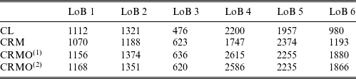
6.1 Comparisons to machine learning techniques and individual claims modelling

As mentioned in the beginning of Section 6, the simulated data used here are also used in Gabrielli et al. (Reference Gabrielli, Richman and Wüthrich2020), Lindholm et al. (Reference Lindholm, Lindskog and Wahl2020) where machine learning techniques are used to learn a general representation of the $\psi_{ijk}$ :s and $\nu_{ij}$ :s (or corresponding quantities) using feed-forward neural networks (NNs) and gradient boosting machines (GBMs). In Table 4, the CRMO⁽¹⁾ is compared with an NN version and a GBM version of the CRM, see Lindholm et al. (Reference Lindholm, Lindskog and Wahl2020) for details concerning the NN and GBM models. From Table 4 it is seen that by using the CRMO with canonical link-functions and the parametrisations (6.1)–(6.4), not using any interactions, the CRMO results are not too far off from those obtained using more flexible machine learning techniques.

Further, the present modelling approach builds on that from, for example, Verrall et al. (Reference Verrall, Nielsen and Jessen2010), Wahl et al. (Reference Wahl, Lindholm and Verrall2019), which makes use of that the underlying stochastic processes allows for preserving various desirable properties when aggregating claim payments and claim counts. Another approach is to instead consider individual claims modelling directly, which naturally allows for closing of claims. One such model that has been evaluated on publicly available data generated using the procedure from Gabrielli and Wüthrich (Reference Gabrielli and Wüthrich2018) is the semi-Markov model introduced in Bettonville et al. (Reference Bettonville, d’Oultremont, Denuit, Trufin and Van Oirbeek2020), which allows for claim closings, but no re-openings. The data used in Bettonville et al. (Reference Bettonville, d’Oultremont, Denuit, Trufin and Van Oirbeek2020) differ from the previously used six LoBs, here a single LoB with approximately 50,000 claims is used, but we refer to Bettonville et al. (Reference Bettonville, d’Oultremont, Denuit, Trufin and Van Oirbeek2020) for more details. The results for the model from Bettonville et al. (Reference Bettonville, d’Oultremont, Denuit, Trufin and Van Oirbeek2020) are given in Table 3 together with the CRMO⁽¹⁾ model.

Table 3

Reserve predictions together with relative model performance for data and model used in Bettonville et al. (Reference Bettonville, d’Oultremont, Denuit, Trufin and Van Oirbeek2020). CRMO⁽¹⁾ is fitted using $\mathcal{N}_0$ and $\mathcal{X}_0$ data, while CRMO^(*) uses out-of-sample payment data for parameter estimation, but uses observed counts from $\mathcal{N}_0$ for prediction.

Table 4.

Reserve predictions together with relative model performance defined as $\frac{R}{\widehat{R}}-1$ for the model fitted to $\mathcal{N}_0^+$ (CRMO⁽¹⁾), as compared to CRM models fitted using gradient boosting machines (GBMs) and neural networks (NNs) from Lindholm et al. (Reference Lindholm, Lindskog and Wahl2020). The smallest absolute residual is marked with a box. The GBM and NN results are found in 4 in Lindholm et al. (Reference Lindholm, Lindskog and Wahl2020), together with detailed model descriptions.

It is here seen that both models perform rather poorly (including standard chain-ladder), but as commented on in Bettonville et al. (Reference Bettonville, d’Oultremont, Denuit, Trufin and Van Oirbeek2020), a closer inspection of the data reveals a number of large outliers. Without going into details concerning outliers, by instead of estimating $\boldsymbol{\theta}$ based on future data, but making predictions based on the observed number of open claims, the CRMO performance is greatly improved. This model is denoted CRMO^(*) in Table 3, and the results for CRMO^(*) indicate that the underlying model structure of the CRMO is sufficiently flexible and accurate in this situation as well. It should, however, be stressed that the result for CRMO^(*) is not to be compared to the Bettonville et al. (Reference Bettonville, d’Oultremont, Denuit, Trufin and Van Oirbeek2020) model results, since the former is fitted to out-of-sample data and the latter is not. This model is merely included to illustrate that the underlying model structure is reasonable, even though the parameter estimates in this application are poor. A final comment concerns the fact that we use a rather large number of parameters in the above GLM formulation of the CRMO. In practice, it would be reasonable to try to reduce the number of parameters by using regularisation techniques.

7 Concluding remarks

The CRMO model is a generalisation of the CRM presented in Wahl et al. (Reference Wahl, Lindholm and Verrall2019), allowing for individual claim openness dynamics, but which can be estimated using aggregated payment and count data. Further, the constructive nature of the modelling allows for explicit and interpretable RBNS and IBNR reserve calculations. In the present paper, estimation of different GLM formulations of the model based on data availability and re-opening assumptions is presented and tested.

The model performs well in the numerical illustrations, with reserve residuals that outperform both the standard CL model and the generalised CRM model. It is also seen that for several simulated LoBs the CRMO performance is on par with machine learning versions of the CRM presented in Lindholm et al. (Reference Lindholm, Lindskog and Wahl2020), see Table 4. A benefit with the CRMO in this comparison is that the CRMO is transparent, that is the structure is completely known, while the machine learning techniques will always contain “black box” elements. Still, similarly as in Lindholm et al. (Reference Lindholm, Lindskog and Wahl2020), it is straightforward to combine the CRMO with NNs or GBMs directly if using $\mathcal{N}_0^+$ data or by using $\mathcal{N}_0$ data together with $p_{ijk} = q_{ijk} $ . For the situation where $p_{ijk} \neq q_{ijk}$ and only $\mathcal{N}_0$ data are available bespoke loss functions are needed, which makes a machine learning technique implementation somewhat more involved.

In order to assess the CRMO model strength compared to other models considering claim openness, a small numerical comparison was made using the data from Bettonville et al. (Reference Bettonville, d’Oultremont, Denuit, Trufin and Van Oirbeek2020). However, the CRMO model fell short to the model presented in Bettonville et al. (Reference Bettonville, d’Oultremont, Denuit, Trufin and Van Oirbeek2020), due to that the realised payment and openness structure in the out-of-sample data was too far off from the data used for parameter estimation. Still, by estimating parameters based on out-of-sample data, something not possible to do in practice, but producing RBNS and IBNR predictions using the actual observed counts, the reserve predictions became close to perfect, see CRMO(^*) in Table 3. This artificial construction can be seen as an indication of that the underlying model structure for claim openness is reasonable even for this data.