


1. Introduction
A solid sphere sedimenting under gravity through a fluid is one of the most important problems in fluid mechanics. Apart from serving as a simplified case of a general family of immersed body flows, the motion of particles through a fluid finds applications in flow and mixing in porous media (Kurzthaler et al. Reference Kurzthaler, Mandal, Bhattacharjee, Löwen, Datta and Stone2021), blood flows (Freund Reference Freund2014), drug delivery (Geng et al. Reference Geng, Dalhaimer, Cai, Tsai, Tewari, Minko and Discher2007), stability of suspensions (Kegel & van Blaaderen Reference Kegel and van Blaaderen2000), and rheology (Bird, Armstrong & Hassager Reference Bird, Armstrong and Hassager1987a). The flow field around the sphere provides an interesting mix of shearing and extensional kinematics. The upstream stagnation point generates biaxial extension and divergence of streamlines around the sphere. There are regions of transient shear flow around the sphere where the shear rate increases between the upstream pole and the equator and subsequently decreases towards the downstream pole. At the downstream stagnation point, the fluid experiences high uniaxial extensional rates, accompanied by long residence times (see figure 1 for upstream/downstream region definition).

Figure 1. Schematic representation of a solid sphere falling in a circular cross-section tube filled with a viscoelastic fluid. The sphere moves downwards and displaces fluid upwards. The fluid flows from the bottom of the tube to the top. Thus the regions below and above the sphere are referred to as upstream and downstream, respectively.
Since the seminal work of Sir George G. Stokes in 1851 (Stokes Reference Stokes1851), it is well-known that the flow profile around an isolated, slowly sedimenting sphere in a Newtonian fluid exhibits both fore-and-aft and axial symmetry. For Newtonian fluids, these symmetries break as the particle settling velocity is increased, and inertia comes into play (Natarajan & Acrivos Reference Natarajan and Acrivos1993). For viscoelastic fluids, the situation is fundamentally different. Viscoelastic fluids usually possess microstructures composed of macromolecules, such as synthetic polymer chains, DNA/RNA and/or proteins. Even for slow flows, where inertia is negligible, flow-induced microscale events (e.g. macromolecular interactions, chain unravelling and stretch) give rise to macroscopic elasticity and nonlinear flow phenomena during the sphere sedimentation (McKinley Reference McKinley, De Kee and Chhabra2002; Chhabra Reference Chhabra2006; D'Avino & Maffettone Reference D'Avino and Maffettone2015; Zenit & Feng Reference Zenit and Feng2018). These phenomena include the development of a slowly decaying high-velocity region downstream of the sphere, the so-called extended wake (Arigo et al. Reference Arigo, Rajagopalan, Shapley and McKinley1995; Fabris, Muller & Liepmann Reference Fabris, Muller and Liepmann1999), or the appearance of a negative wake, where the fluid behind the sphere flows in the upward direction, against gravity, away from the falling sphere (Bisgaard Reference Bisgaard1983; Arigo & McKinley Reference Arigo and McKinley1998). The magnitude and type of elastic wake depends on the macromolecular extensibility (Harlen Reference Harlen2002). The sphere usually reaches a terminal settling velocity (Arigo et al. Reference Arigo, Rajagopalan, Shapley and McKinley1995; Solomon & Muller Reference Solomon and Muller1996; Arigo & McKinley Reference Arigo and McKinley1998; Fabris et al. Reference Fabris, Muller and Liepmann1999). Few cases with oscillatory settling velocities have been reported (Jayaraman & Belmonte Reference Jayaraman and Belmonte2003; Chen & Rothstein Reference Chen and Rothstein2004). Nevertheless, existing experimental, theoretical and computational works suggest that the flow remains axisymmetric, regardless of different flow conditions and viscoelastic properties of the fluids.
Given the symmetry-breaking patterns that arise beyond a critical flow rate in flows of viscoelastic fluids in planar geometries (Arratia et al. Reference Arratia, Thomas, Diorio and Gollub2006; Poole, Alves & Oliveira Reference Poole, Alves and Oliveira2007; Haward et al. Reference Haward, Kitajima, Toda-Peters, Takahashi and Shen2019; Varchanis et al. Reference Varchanis, Hopkins, Shen, Tsamopoulos and Haward2020a, Reference Varchanis, Haward, Hopkins, Tsamopoulos and Shen2022a) and the axisymmetry breaking in bubbles rising in viscoelastic fluids (Hassager Reference Hassager1979; Moschopoulos et al. Reference Moschopoulos, Spyridakis, Dimakopoulos and Tsamopoulos2024), one would expect axisymmetry around a falling sphere to break with increasing elasticity of the fluid. However, in the absence of quantitative data, this assumption cannot be verified. High-resolution three-dimensional velocity (e.g. particle image velocimetry) and stress field (e.g. flow-induced birefringence) measurements are difficult to obtain due to challenges in flow visualizations. Existing analytical attempts refer to axisymmetric and weakly elastic flows (Housiadas & Tanner Reference Housiadas and Tanner2016). Thus a numerical solution of the governing equations is necessary. However, the strong tensile stresses that develop downstream of the moving sphere cause loss of numerical convergence and trigger the well-known high Weissenberg number problem (Alves, Oliveira & Pinho Reference Alves, Oliveira and Pinho2021). Moreover, three-dimensional viscoelastic flow simulations require extraordinary computational cost and time to obtain accurate solutions. Consequently, computational works are restricted to axisymmetric simulations (Jin, Phan-Thien & Tanner Reference Jin, Phan-Thien and Tanner1991; Lunsmann et al. Reference Lunsmann, Genieser, Armstrong and Brown1993; Rasmussen & Hassager Reference Rasmussen and Hassager1993; Owens & Phillips Reference Owens and Phillips1996) or low settling velocities (Knechtges Reference Knechtges2015), and have never captured non-axisymmetric flow profiles and elastic instabilities around the falling sphere.
2. Problem formulation
In this work, we present a simple model that captures the essential physics during the settling of a solid sphere (density  $\rho _s$, radius $R_s$) through a cylindrical tube (radius $R_t$) filled with an incompressible viscoelastic fluid (density $\rho _f$, relaxation time $\lambda$, polymer viscosity $\eta _p$, solvent viscosity $\eta _s$, and total viscosity $\eta = \eta _p + \eta _s$). We assume steady, three-dimensional flow. The tube height is long compared to $R_s$, allowing the establishment of a steady settling velocity $U_s$ (figure 1). Cartesian coordinates are employed, with the origin placed at the centre of the sphere. This implies a reference frame in which the sphere is stationary, and the tube (along with the fluid far from the sphere) is moving at a uniform velocity $U_s \boldsymbol {e}_z$, where $\boldsymbol {e}_i$ the unit normal vector in the $i$th direction. The gravitational acceleration is given as $-g\boldsymbol {e}_z$. The sphere does not rotate around any axis, and its centre is located on the symmetry axis of the tube. We scale all lengths, velocities and stress components with $R_s$, $U_s$ and $\eta U_s/R_s$, respectively. The Reynolds number ( $Re = \rho _f U_s R_s / \eta$) compares inertial to viscous forces. In typical experiments (Arigo et al. Reference Arigo, Rajagopalan, Shapley and McKinley1995; Solomon & Muller Reference Solomon and Muller1996; Arigo & McKinley Reference Arigo and McKinley1998; Fabris et al. Reference Fabris, Muller and Liepmann1999; Jayaraman & Belmonte Reference Jayaraman and Belmonte2003; Chen & Rothstein Reference Chen and Rothstein2004) with small, high-density spheres ( $R_s < 3\,{\rm mm}$, $\rho _s > 2500\, {\rm kg}\,{\rm m}^{-3}$) and viscous fluids ( $\eta >1$ Pa s), inertia can be neglected ( $Re<0.03$). Hence in simulations we set $Re\equiv 0$. The Weissenberg number ( $Wi = \lambda U_s / R_s$) compares elastic to viscous forces and is directly related to the settling velocity. We also define the solvent to total viscosity ratio $\beta = \eta _s/\eta$, and the geometrical blockage ratio $B_R = R_s^2/R_t^2$. Thus the physical problem is governed by only three parameters, $Wi$,
$Wi$,  $\beta$ and $B_R$.
The fluid rheology is described by the Oldroyd-B model, which reproduces the basic experimentally measured properties of viscoelastic fluids (memory effects, development of normal stresses under shear, extension hardening) with minimal parameters. According to the kinetic theory (Bird et al. Reference Bird, Curtiss, Armstrong and Hassager1987b), macromolecules are modelled as non-interacting, Hookean dumbbells in a Newtonian solvent. Under homogeneous steady shear, the model predicts a constant shear viscosity,  $\eta _{sh} = \eta _0$, for any value of the shear rate (Bird et al. Reference Bird, Armstrong and Hassager1987a). However, under transient shearing, the model predicts shear thinning/thickening effects (Varchanis et al. Reference Varchanis, Tsamopoulos, Shen and Haward2022b). Under homogeneous steady uniaxial extension, the model predicts an extensional viscosity, $\eta _{e} = 3\eta _s + 3\eta _p/[(1-2\lambda \dot \varepsilon )(1+\lambda \dot \varepsilon )]$, which is nearly constant for low extension rates $\dot \varepsilon$, but becomes infinite for $\dot \varepsilon \geq 1/(2\lambda )$ (Bird et al. Reference Bird, Armstrong and Hassager1987a). The solvent to total viscosity ratio $\beta$ is related to the concentration of macromolecules. Fluids with $\beta \rightarrow 0$ correspond to concentrated solutions with transient shear thinning/thickening effects (Varchanis et al. Reference Varchanis, Tsamopoulos, Shen and Haward2022b), while fluids with $\beta \rightarrow 1$ correspond to ultra-dilute solutions with Newtonian-like shear response (Varchanis et al. Reference Varchanis, Tsamopoulos, Shen and Haward2022b). For any $\beta$ value, strong extension hardening takes place around stagnation points as $\dot \varepsilon =1/(2\lambda )$ is approached.
3. Governing equations and boundary conditions
The non-Newtonian flow is described by the incompressible and isothermal Cauchy equations coupled with the Oldroyd-B constitutive equation, which accounts for the contribution of non-Newtonian stresses. Neglecting inertia, the forms of the dimensionless continuity, momentum and constitutive equations are expressed, respectively, as
 \begin{gather} \boldsymbol{\nabla} \boldsymbol{\cdot} \boldsymbol{u} = 0, \end{gather}
 \begin{gather} \boldsymbol{\nabla} \boldsymbol{\cdot} ( - P \boldsymbol{\mathsf{I}} + \boldsymbol{\mathsf{T}} + 2\beta\boldsymbol{\mathsf{D}} ) = \boldsymbol{0} , \end{gather}
 \begin{gather} Wi\,\overset{\triangledown}{\boldsymbol{\mathsf{T}}} + \boldsymbol{\mathsf{T}} = 2(1-\beta) \boldsymbol{\mathsf{D}}, \end{gather}
where  $\boldsymbol {u}$ is the velocity vector, $P$ is thermodynamic pressure, and $2\boldsymbol{\mathsf{D}} = \boldsymbol {\nabla }\boldsymbol {u} + (\boldsymbol {\nabla }\boldsymbol {u})^{\rm T}$ is the deformation rate tensor. The inverted triangle above the stress tensor $\boldsymbol{\mathsf{T}}$ in (3.3) denotes the upper convected derivative, $\overset {\triangledown }{\boldsymbol{\mathsf{T}}} = {\partial \boldsymbol{\mathsf{T}}}/{\partial t} + \boldsymbol {u} \boldsymbol {\cdot } \boldsymbol {\nabla }\boldsymbol{\mathsf{T}} - (\boldsymbol {\nabla }\boldsymbol {u})^{\rm T} \boldsymbol {\cdot } \boldsymbol{\mathsf{T}} - {\boldsymbol{\mathsf{T}}} \boldsymbol {\cdot } \boldsymbol {\nabla }\boldsymbol {u}$. No-slip ( $\boldsymbol {n} \boldsymbol {\cdot } \boldsymbol {u} = 0$) and no-penetration ( $\boldsymbol {t} \boldsymbol {\cdot } \boldsymbol {u} = 0$) conditions are imposed on the sphere surface. Note that $\boldsymbol {n}$ and $\boldsymbol {t}$ denote the normal and tangent unit vectors on the sphere surface, respectively. On the tube wall ( $x^2 + y^2 = R_t^2$) and inflow boundary ( $z = - 25$), we impose $\boldsymbol {u} = [0,0,1]$. Finally, on the outflow boundary ( $z = 25$), we apply the open boundary condition (Papanastasiou, Malamataris & Ellwood Reference Papanastasiou, Malamataris and Ellwood1992). According to the open boundary condition, the fluid velocities and stresses are not imposed at the outflow boundary but are calculated from the weak form of the equations for the velocity unknowns (extrapolated from the bulk). We have verified that the computational domain height ( $H_c=50$) does not affect our predictions in any way.
4. Characterized quantities
The results that follow will be presented in terms of the drag force acting on the sphere  $\boldsymbol{\mathsf{F}}_D$ and the flow asymmetry parameter $I$. The dimensionless drag force exerted on the sphere is defined as
 \begin{equation} \boldsymbol{\mathsf{F}}_D = \int_S \boldsymbol{n} \boldsymbol{\cdot} [ - P \boldsymbol{\mathsf{I}} + \boldsymbol{\mathsf{T}} + 2\beta\boldsymbol{\mathsf{D}} ]\,{\rm d}S , \end{equation}
where  $S$ is the dimensionless area of the sphere surface.
The flow asymmetry parameter is defined as
 \begin{equation} I = \int_V \vert u_\phi \vert \,{\rm d}V, \end{equation}
where  $V$ is the dimensionless volume occupied by the fluid, and $u_\phi = \boldsymbol {u} \boldsymbol {\cdot } \boldsymbol {e}_{\phi }$ is the dimensionless azimuthal velocity. Here, $I=0$ indicates axisymmetric flow; when $I>0$, azimuthal velocities arise and the flow becomes non-axisymmetric.
5. Computational method
The governing equations (3.1)–(3.3) are discretized and solved using the Petrov–Galerkin stabilized finite element method for viscoelastic flows (PEGAFEM-V) (Varchanis et al. Reference Varchanis, Syrakos, Dimakopoulos and Tsamopoulos2019, Reference Varchanis, Syrakos, Dimakopoulos and Tsamopoulos2020b; Varchanis & Tsamopoulos Reference Varchanis and Tsamopoulos2022). The positive definiteness of the conformation tensor  $\boldsymbol{\mathsf{C}}=Wi\,\boldsymbol{\mathsf{T}}/(1-\beta )+\boldsymbol{\mathsf{I}}$ is enforced by a symmetric square root reformulation of (3.3) (Balci et al. Reference Balci, Thomases, Renardy and Doering2011). All flow variables ( $\boldsymbol {u}, P, \sqrt {\boldsymbol{\mathsf{C}}}$) are interpolated by linear polynomials, and the computational mesh is composed of structured tetrahedral elements. The three-dimensional mesh is created by revolution of a two-dimensional mesh (quadrilateral elements) around the $z$-axis and appropriate tetrahedralization of the resulting hexahedral and prismatic elements. This handling guarantees that the mesh is always axisymmetric (figure 2a). Moreover, the mesh is highly refined around the downstream stagnation point (figure 2b). A mesh convergence study is given in figure 2(c). Additional mesh convergence and validation studies can be found in Appendices A and B. Mesh M2 (see table 1) was used in all direct steady-state simulations presented in the main text.

Figure 2. (a,b) Indicative mesh views at the  $z=0$ and $x=0$ planes, respectively. Only parts of the mesh are shown. This mesh is created for visualization purposes only and is much coarser than meshes M1, M2 and M3 (table 1). (c) The effect of mesh refinement on the asymmetry parameter for $\beta = 0.1$ and $B_R = 0.25$. The solution branches are obtained by direct steady-state simulations assuming symmetry across the $x=0$ and $y=0$ planes.
Table 1. Main characteristics of the meshes used in this study. Here,  $h_e$ denotes the dimensionless element ‘length’ at the rear pole of the sphere. Element and node numbers refer to one-quarter of the geometry, assuming symmetry across the $x=0$ and $y=0$ planes.

For a given set of flow parameters ( $Wi, \beta, B_R$), we first perform transient simulations. The initial conditions are $\boldsymbol {u} = \boldsymbol {0}$, $\boldsymbol {P} = 0$ and $\sqrt {\boldsymbol{\mathsf{C}}} = \boldsymbol{\mathsf{I}}$. At time $t=0^+$, a velocity $\boldsymbol {u} = [0,0,1-{\rm e}^{-t}]$ is applied on the tube wall and inflow boundary. For high $Wi$, transient simulations starting from equilibrium are very challenging and may lead to divergence of our numerical scheme. In cases where divergence of our time marching scheme is encountered, we use the last steady state obtained from convergent transient simulations, $Wi_p$, as the initial condition, and gradually increase the Weissenberg number according to the expression $Wi = Wi_p + {\rm d}Wi\,(1-{\rm e}^{-t/{\rm d}Wi})$, where ${\rm d}Wi$ is the increment in $Wi$.
$Wi$.
Time integration of (3.1)–(3.3) is performed using a fully implicit, second-order backward finite difference time integration scheme (see Varchanis et al. (Reference Varchanis, Syrakos, Dimakopoulos and Tsamopoulos2019) for details). The time step for all transient calculations is  ${\rm d}t = 0.02$. A time step convergence study is given in Appendix A. In all transient simulations, we solve the whole geometry by patching four M1 meshes. These transient simulations are extremely time-consuming, and only mesh M1 was used.
The steady states obtained by the transient simulations are then interpolated to mesh M2 and used as an initial guess for direct steady-state simulations at the same values of the flow parameters. Depending on the resulting mode of instability, we take advantage of possible planar symmetries to reduce the computational cost. For example, when a transient simulation of the whole geometry yields a four-lobed solution, direct steady-state simulations are performed by solving only a quarter of the geometry, assuming flow symmetry across the  $x=0$ and $y=0$ planes. In the direct steady-state simulations, the time derivative in the constitutive equation (3.3) is neglected, and $Wi$ is altered gradually; this process is called parameter continuation. Finally, the families of steady solution branches in the parametric space are traced by a pseudo-arc-length continuation algorithm (see Varchanis, Dimakopoulos & Tsamopoulos (Reference Varchanis, Dimakopoulos and Tsamopoulos2017) for details). This handling enables efficient tracking of regular and saddle-node bifurcations in the parametric space. Furthermore, using the bifurcation theory and the fact that parameter continuation starts from a steady state obtained by transient simulations, we can determine whether a solution branch is stable or unstable.
6. Results and discussion
We consider a base case of a sphere falling in a tube with  $R_t = 2R_s$ ( $B_R = 0.25$), filled with a semi-dilute solution ( $\beta = 0.1$). Starting from low $Wi$ values (figures 3a,b), the flow reaches an axisymmetric steady state, exhibiting an extended elastic wake that intensifies with increasing $Wi$. For $Wi>Wi_c\approx 1.55$, axisymmetric states become unstable, and a regular bifurcation occurs (figure 3a). Flow profiles suddenly change, and a four-lobed solution emerges (figure 3c). A right angle is formed by each pair of neighbouring lobes, and the flow exhibits two planar symmetries, each one with respect to the plane formed by opposing lobes.

Figure 3. (a) Asymmetry parameter  $I$ versus Weissenberg number $Wi$ for $\beta = 0.1$ and $B_R = 0.25$. (b,c) Iso-surfaces of the dimensionless stress tensor trace ( $\text {tr}(\boldsymbol{\mathsf{T}})=20$) with superimposed dimensionless velocity magnitude ( $|\boldsymbol {u}|$) contours for $Wi=2$, on the (b) unstable and (c) stable solution branches. (d,e) Contours of dimensionless velocity magnitude and stress tensor trace on the plane $z=1.4$ for $Wi=2$, $\beta =0.1$ and $B_R=0.25$, on the (d) unstable and (e) stable solution branches. The solution branches are obtained by direct steady-state simulations assuming symmetry across the $x=0$ and $y=0$ planes. The stability of the branches is determined by a transient simulation of the whole geometry for $Wi = 2$.
An examination of the bifurcated solution in figure 3(c) reveals that axisymmetry is broken only downstream of the sphere; the flow upstream of the sphere is still axisymmetric (observe contours around the upstream pole in figures 3b,c). Obviously, this non-axisymmetric instability is strongly related to the downstream stagnation point. To get a better insight into the flow and deformation profiles around the rear pole, we plot in figures 3(d,e) the velocity magnitude and stress tensor trace contours on the plane  $z=1.4$, for $Wi=2$. Starting with the unstable, axisymmetric solution, we observe that uniaxial extension takes place around the rear stagnation point; the radial velocity is proportional to the radial coordinate $r=\sqrt {x^2+y^2}$, and the stresses are uniformly distributed peripherally of the sphere. In the stable, bifurcated solution, extension is constrained inside the lobes, downstream of the sphere. We observe the formation of two sheets, aligned with each pair of opposing lobes, where planar extension takes place. Clearly, planar extension becomes favourable over uniaxial extension, beyond a critical value of the settling velocity.
It is also worth examining the drag force on the particle. Figure 4(a) presents the dimensionless drag force versus  $Wi$. Beyond $Wi_c$, the drag force is higher in the stable bifurcated state, meaning that more power is dissipated and a lower terminal velocity ( $U_s$) is reached, compared to the unstable axisymmetric case. Consequently, this bifurcation drives the system to a higher energy dissipation rate. This observation contradicts patterns observed in steady elastic instabilities around planar stagnation points (Poole et al. Reference Poole, Alves and Oliveira2007; Varchanis et al. Reference Varchanis, Hopkins, Shen, Tsamopoulos and Haward2020a), where the stable asymmetric solutions dissipate less power than the unstable symmetric ones. Our finding is unexpected because the transition of the system to lower energy dissipation rates and the related ‘stress relief mechanism’ could partially explain such instabilities (Poole et al. Reference Poole, Alves and Oliveira2007). However, the minimum energy principle strictly holds under equilibrium, and does not necessarily hold in out-of-equilibrium states (e.g. flowing systems). A representative example is the inertial breakage of axisymmetry around a sphere falling in a Newtonian fluid, where the stable non-axisymmetric solutions dissipate more power (Jenny, Dušek & Bouchet Reference Jenny, Dušek and Bouchet2004) than the unstable axisymmetric ones, in complete analogy to the present observations.

Figure 4. (a) Dimensionless drag force  $\boldsymbol{\mathsf{F}}_D$ versus Weissenberg number $Wi$ for $\beta = 0.1$ and $B_R = 0.25$. (b) Asymmetry parameter $I$ versus Weissenberg number $Wi$ for $\beta = 0, 0.1, 0.2, 0.4$ and $B_R = 0.25$. (c) Asymmetry parameter $I$ versus Weissenberg number $Wi$ for $\beta = 0.1$ and $R_s/R_t = 1/1.4, 1/2, 1/2.8, 1/4$ ( $B_R \approx 0.062, 0.128, 0.25, 0.51$). (d) Reciprocal critical Weissenberg number $1/Wi_c$ versus blockage ratio $B_R$. All solution branches are obtained by direct steady-state simulations assuming symmetry across the $x=0$ and $y=0$ planes.
To understand the physics of this flow instability, we investigate the influence of the rheological and geometrical parameters in our model. We start with the rheological parameter,  $\beta$, which mainly governs the shear response of the fluid (Varchanis et al. Reference Varchanis, Tsamopoulos, Shen and Haward2022b). Note that the steady extensional viscosity is relatively insensitive to $\beta$. For $\dot \varepsilon \geq 1/(2\lambda )$ (necessarily true when the instability occurs) and various $\beta$ values, differences in the startup extensional viscosity will be observed only at early times. As the stresses evolve, any solvent contribution will become negligible compared to the exponentially growing tensile stresses. Residence times around stagnation points are long. Thus the role of $\beta$ in extension-dominated regions is negligible. However, $\beta$ plays a crucial role in shear-dominated regions (after the front and before the rear pole of the sphere). As shown by Varchanis et al. (Reference Varchanis, Tsamopoulos, Shen and Haward2022b), low $\beta$ values can create apparent shear thinning effects in shear-dominated flows, even when using the Oldroyd-B model. Thus in shear-dominated regions, low values of $\beta$ allow variations in the local viscosity, while high values of $\beta$ imply a Newtonian-like response with almost constant local viscosity. Figure 4(b) shows the effect of varying $\beta$ for $B_R = 0.25$. As $\beta$ is increased (i.e. local viscosity variations in shear-dominated regions are suppressed), the onset $Wi_c$ for asymmetry increases. In addition, for a given $Wi$, increasing $\beta$ tends to reduce the asymmetry magnitude. Hence we can conclude that local viscosity variations in the shear-dominated flow regions around the sphere promote non-axisymmetric flow profiles. We believe that this steady elastic instability will completely vanish for sufficiently large values of $\beta$, in analogy with the steady elastic instabilities in the cross-slot channel (Xi & Graham Reference Xi and Graham2009; Canossi, Mompean & Berti Reference Canossi, Mompean and Berti2020; Yokokoji et al. Reference Yokokoji, Varchanis, Shen and Haward2024) and the flow past a cylinder in a confined channel (Varchanis et al. Reference Varchanis, Hopkins, Shen, Tsamopoulos and Haward2020a). We do not present solutions for $\beta > 0.4$ because the stress boundary layers around the rear stagnation point become very thin, and reliable solutions cannot be obtained with the present spatial discretization. In accordance with our observations, increasing $\beta$ has been found to diminish non-axisymmetric solutions in Taylor–Couette flows (Avgousti & Beris Reference Avgousti and Beris1993).
Next, we proceed to the effect of the geometrical parameter  $B_R$. Figure 4(c) shows the effect of varying $B_R$ for $\beta = 0.1$. Increasing $B_R$ decreases the onset $Wi_c$ for asymmetry, and for a given $Wi$, increases the asymmetry magnitude. This happens because as $B_R$ increases, the extension rate at the rear stagnation point becomes considerably larger than the characteristic extension rate ( $U_s/R_s$), and extension hardening comes into play at lower $Wi$ values. Thus extension hardening also promotes non-axisymmetric flow states.
The  $B_R$ parametric analysis also provides important information about the onset of this flow phenomenon. A well-known criterion for the onset of purely elastic (i.e. inertialess) flow instabilities proposed by McKinley, Pakdel & Öztekin (Reference McKinley, Pakdel and Öztekin1996) considers the generation of elastic tensile stresses along curving streamlines and can be expressed as
 \begin{equation} \frac{\lambda U}{\mathcal{R}}\,\frac{\tau_{ss}}{\eta \dot\gamma} = M^2, \end{equation}
where  $\mathcal {R}$ is the characteristic radius of curvature of the streamline, $\tau _{ss}$ is the streamwise tensile stress, and $\dot \gamma$ is the local deformation rate. When, at some locality in the flow field, the left-hand side of (6.1) exceeds a critical value $M_{c}^2$, the flow becomes prone to instability originating from that location. For flows past a sphere falling in a tube, simple scaling arguments for the values of $\mathcal {R}$, $\tau _{ss}$ and $\dot \gamma$ around the downstream stagnation point (McKinley et al. Reference McKinley, Pakdel and Öztekin1996) indicate that flow instability will arise for
 \begin{equation} \frac{1}{Wi_c} = \frac{1+a B_R}{M_{c}}, \end{equation}
where  $a$ is a numerical constant that is determined from experiments or simulations. Our computational results for $B_R$ versus $1/Wi_c$ (figure 4d) follow the predicted linear scaling very well. Fitting (6.2) to the data in figure 4(d) yields $a = 5.5$ and $M_c = 3.6$ (with $M_c$ being consistent with values reported in other purely elastic instabilities; McKinley et al. Reference McKinley, Pakdel and Öztekin1996). These arguments strongly suggest that the initial perturbation to the flow field that drives the breakage of axisymmetry is due to the accumulation of elastic tensile stresses along the strongly curving streamlines passing around the downstream stagnation point.
Keeping all these points in mind, we propose a mechanism for the onset and subsequent evolution of this flow instability. At low settling velocities ( $Wi< Wi_c$), the extensionally thickened fluid downstream of the sphere lies axisymmetrically around the $z$-axis, and the local viscosity does not vary azimuthally. At the onset of critical conditions ( $Wi \approx Wi_c$), the accumulation of elastic tensile stresses along the highly curving streamlines around the rear stagnation point causes a disturbance that perturbs the elastic wake randomly in the radial direction (figure 5a). Due to the axisymmetric nature of the geometry, the radial deflection of the elastic wake generates non-axisymmetric disturbances downstream of the sphere. These non-axisymmetric disturbances create variations in the deformation rate and introduce shear contributions peripherally of the rear stagnation point. The presence of shear deformations will give rise to increased and reduced flow resistance paths. The local viscosity will decrease in regions with increased shear deformations (indentations), while it will remain high in extension-dominated flow regions (lobes). This flow resistance inequality will push more fluid into the indentations, amplify the azimuthal disturbances, and eventually lead to the establishment of the non-axisymmetric steady state.

Figure 5. (a) Schematic illustration of the destabilization mechanism for non-axisymmetric flow of viscoelastic fluids past a sphere. Coloured regions are indicative of the stress tensor trace obtained from numerical simulations. (b,c) Contours of the dimensionless stress tensor trace with superimposed streamlines at (b)  $\phi = 3{\rm \pi} /4$ (red sheet), and (c) $\phi = {\rm \pi}/2$ (blue sheet), for $Wi=2$, $\beta = 0.1$ and $B_R=0.25$. The streamlines in (b,c) pass from the points $(r,\phi, z) = (0.1, 3{\rm \pi} /4, -2)$ and $(0.1, {\rm \pi}/2, -2)$, respectively. (d,e) Translucent iso-surfaces of the dimensionless stress tensor trace ( $\text {tr}(\boldsymbol{\mathsf{T}})=20$) along with red iso-surfaces of the spatial variation of parameter $M$ (
$M$ ( $M=4.5$) for $Wi=2$, $\beta = 0.1$ and $B_R=0.25$ on the (d) unstable and (e) stable solution branches.
In this new flow configuration, the flow is slow and extension-dominated (high stresses) inside the lobes, while it is fast and shear-dominated (low stresses) inside the indentations. Additionally, streamline curvature is minimized inside the lobes and maximized inside the indentations. This high-stress/low-streamline curvature combination inside the lobes (figure 5b) along with the low-stress/high-streamline curvature combination inside the indentations (figure 5c) leads to a more topologically stable form, which is resistant to flow perturbations. Our arguments are additionally supported by plotting the spatial variation of  $M$ in (6.1) (Cruz et al. Reference Cruz, Poole, Afonso, Pinho, Oliveira and Alves2016) for two steady states with the same flow parameter values ( $Wi=2$, $\beta = 0.1$, $B_R = 0.25$) on the stable and unstable solution branches, respectively (see figures 5d,e). On the unstable branch, the large volume of fluid that passes through the red toroidal surface (red iso-surface for $M=4.5$ in figure 5d) is prone to elasticity-driven flow perturbations, leading to a topologically unstable axisymmetric form. In the stable branch, the volume of fluid that is prone to perturbations is very small and localized at each lobe tip (red iso-surfaces for $M=4.5$ in figure 5c), leading to topologically stable and observable patterns.
One last question that must be answered is why the flow bifurcates to four-lobed shapes. We simulated many cases with various numbers of elements around the sphere, which could presumably trigger solutions with different lobe numbers (e.g. using 81 elements in the  $\phi$-direction would favour three-lobed solutions), but we always obtained four-lobed stable solutions. We believe that shapes with point symmetry are favoured over shapes without it because point symmetry can be seen as reminiscent of axisymmetry (the previous state of the system). According to this idea, we expect only even-number-lobed shapes behind perfectly spherical particles falling in perfectly circular cross-section tubes. However, a two-lobed shape is inconsistent with our physical mechanism because it leads to a single sheet of planar extension downstream of the sphere. This disallows the formation of low-resistance, shear-dominated paths and the transition of the system to more topologically stable forms. On the other hand, four is the smallest lobe number exhibiting point symmetry and allowing the formation of low-resistance paths; this is why we observe four-lobed shapes. Nevertheless, we cannot exclude the emergence of odd-number-lobed shapes in non-axisymmetric geometries (e.g. particles and/or tubes with surface defects).
Finally, we examine what happens at higher  $Wi$ values. Figure 6(a) presents $I$ versus $Wi$ for our base case. After the regular bifurcation at $Wi\approx 1.55$ and the emergence of four-lobed shapes, the asymmetry parameter increases with increasing $Wi$. However, at $Wi\approx 2.7$, we observe two successive saddle-node bifurcations, defining a hysteresis loop, and giving rise to eight-lobed shapes (see figure 6d). After the first saddle-node bifurcation at $Wi \approx 2.7$, each lobe tip is split into two new lobes, and low-resistance paths emerge in between the pairs of new lobes. We interpret this transition using the physical mechanism proposed for the breakage of azimuthal symmetry. Tensile stresses around lobe tips grow exponentially with $Wi$ (the flow is extension-dominated at these regions). Even if streamline curvature remains constant around these points, $M$ increases proportionally with the square root of tensile stresses (6.1) and $Wi$. At some $Wi_{c,2}$ and
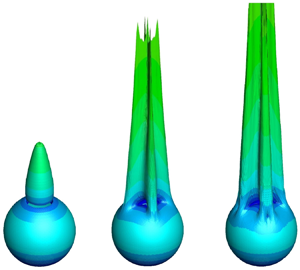
  $M_{c,2}$, perturbations caused by tensile stresses along curving streamlines destabilize the flow locally, and following the same events described in previous paragraphs, the extension-dominated lobe tip evolves into a more topologically stable form. The localities where perturbations originated from (figure 5e) become shear-dominated (high-curvature/low-stress combination) and extension is ‘diffused’ to the new lobes (low-curvature/high-stress combination), leading to the eight-lobed shape. Interestingly, this eight-lobed structure resembles experimentally measured shapes (Haward Reference Haward1998) behind steel spheres falling in high molecular weight polystyrene (HMWPS) using flow-induced birefringence (figure 6f). Although the Oldroyd-B model cannot quantitatively describe the rheology of HMWPS solutions, a visual comparison between the simulated (figure 6e) and experimental (figure 6f) stress fields reveals a nice qualitative agreement and validates our toy model.

Figure 6. (a) Asymmetry parameter versus Weissenberg number for  $\beta = 0.1$ and $B_R = 0.25$. The solution branches are obtained by direct steady-state simulations assuming symmetry across the $x=0$ and $y=0$ planes. The stability of the branches is determined by transient simulations of the whole geometry for $Wi = 2$ and $3$. (b i,c i,d i) Iso-surfaces of the dimensionless stress tensor trace ( $\text {tr}(\boldsymbol{\mathsf{T}})=20$) with superimposed dimensionless velocity magnitude ( $\lvert \boldsymbol {u} \rvert$) contours for (b) $Wi=1.3$, (c) $Wi=2$, (d) $Wi=2.7$ on the stable solution branch ( $\beta =0.1$, $B_R=0.25$). (b ii,c ii,d ii) Contours of the dimensionless stress tensor trace on the plane $z=1.4$ for (b) $Wi=1.3$, (c) $Wi=2$, (d) $Wi=2.7$ on the stable solution branch ( $\beta =0.1$, $B_R=0.25$). (e,f) Visual comparison between iso-surfaces of the dimensionless stress tensor trace ( $\text {tr}(\boldsymbol{\mathsf{T}})=50$) obtained from simulations ( $Wi=3.5$, $\beta =0.1$, $B_R=0.25$) and experimentally measured flow-induced birefringence for a steel ball falling in a polystyrene solution ( $Wi \approx 3.5$) (Haward Reference Haward1998). (g) Elongation of viscoelastic fluid filaments: (g i,ii) side views for increasing strain, (g iii,iv) bottom views through a glass endplate for increasing strain. Reproduced with permission from Anna, Spiegelberg & McKinley (Reference Anna, Spiegelberg and McKinley1997). Copyright 1997, AIP Publishing LLC.
One can envision that the tip-splitting process will continue indefinitely with increasing  $Wi$, and eventually lead to a dendritic, fractal-like structure. Similar fingering instabilities leading to dendritic patterns have been observed in many interfacial flows, such as the invasion of one Newtonian fluid into another (Bischofberger, Ramachandran & Nagel Reference Bischofberger, Ramachandran and Nagel2014), and the decohesion of viscoelastic fluids (or soft media) from flat surfaces (Anna et al. Reference Anna, Spiegelberg and McKinley1997; Bach et al. Reference Bach, Rasmussen, Longin and Hassager2002; Lin et al. Reference Lin, Cohen, Zhang, Yuk, Abeyaratne and Zhao2016). Figure 6(g) presents photos from viscoelastic fluid filament stretching experiments (Anna et al. Reference Anna, Spiegelberg and McKinley1997). A cylindrical sample of polystyrene solution is placed between two plates, and the upper plate is separated at a prescribed velocity from the lower one, which is held still. As the process evolves, a cylindrical fluid column is formed, while side and bottom views of the lower glass endplate are provided (figure 6g). The filament is axisymmetric at low strains. As strain accumulates, non-axisymmetric disturbances arise peripherally of the filament. The intensity of these disturbances maximizes close to the endplate. Initially, the disturbances have a four-lobed shape, but each lobe tip is split as strain increases. The deformation patterns in figure 6(g) greatly resemble the flow profiles behind the sphere (figures 6b–d), and this is not coincidental. If we restrict our analysis very close to the stagnation points, then we can neglect the sphere curvature (flow past a sphere) and the presence of the free surface (filament stretching case). Now, both flow set-ups are identical: fluid detaches from a solid surface, forming a cylindrical ‘stream’ around a stagnation point. The only difference is the limited amount of fluid in the filament case. As the process evolves, the liquid reservoir on the endplate drains, leading to a thinner and faster ‘stream’. The flow is time-dependent, and strain increases monotonically with time. Instead, incoming fluid fuels the stagnation point behind the sphere, a finite amount of strain is accumulated along streamlines passing near that region, and a steady state is established. These arguments strongly suggest that we observe the same elastic instability in both cases and further support our theory.
Finally, it is intuitive to discuss the similar patterns observed in the present inertialess viscoelastic flow and the inertial Newtonian flow past a confined sphere. At low Reynolds numbers, the Newtonian flow is steady and axisymmetric. At  $Re \approx 105$, a regular bifurcation causes the breakage of axisymmetry (Natarajan & Acrivos Reference Natarajan and Acrivos1993) and leads to the formation of a ‘double-thread’ inertial wake (Tomboulides & Orszag Reference Tomboulides and Orszag2000). In this new flow configuration, the flow is steady, and the flow profiles exhibit planar symmetry (Tomboulides & Orszag Reference Tomboulides and Orszag2000). The similarity between the inertialess viscoelastic and inertial Newtonian flows is, therefore, in the loss of the axisymmetric solution stability via a regular bifurcation and the transition of the system to nonaxisymmetric steady states with planar symmetries. However, these systems follow different paths as elasticity and inertia increase. A hysteresis loop at $Wi \approx 2.7$ drives the inertialess viscoelastic system to a new steady state with an eight-lobed elastic wake. In contrast, a Hopf bifurcation at $Re \approx 270$ drives the inertial Newtonian system to time-dependent and eventually chaotic states. We did not examine flow profiles for $Wi > 3$, but we believe that the flow will become time-dependent at higher $Wi$, in analogy with other elastic instabilities around stagnation points (Poole et al. Reference Poole, Alves and Oliveira2007; Varchanis et al. Reference Varchanis, Haward, Hopkins, Tsamopoulos and Shen2022a). Elasticity and inertia are two forces that manifest at different length scales, act in a very different way, and even suppress each other when they are both present in a flow. However, it seems that they can cause similar flow phenomena when only one of them is present. Analogous correlations have been made in the elastic (Poole et al. Reference Poole, Alves and Oliveira2007) versus inertial (Poole, Rocha & Oliveira Reference Poole, Rocha and Oliveira2014) breakage of planar symmetry in a cross-slot flow.
7. Conclusions
To conclude, we have discovered a new viscoelastic fingering instability during the sedimentation of a sphere. The onset and subsequent evolution of the instability depend solely on the interplay between shear and rate-dependent extensional viscosities of the viscoelastic fluid. Our analysis advances the fundamental understanding of the relationship between rheological properties and macroscopically observed phenomena in non-Newtonian flows, and sheds light on the physical mechanisms that trigger elastic fingering instabilities in a wide class of flows, including flows past rigid particles and decohesive flows.
Acknowledgements
The authors acknowledge stimulating discussions with J. Tsamopoulos, G.H. McKinley, and P. Moschopoulos.
Funding
S.V., S.J.H., E.Y. and A.Q.S. gratefully acknowledge the support of the Okinawa Institute of Science and Technology Graduate University (OIST) with subsidy funding from the Cabinet Office, Government of Japan, and also funding from the Japan Society for the Promotion of Science (JSPS, grant nos 21K03884, 22K14184). The authors are grateful for the help and support provided by the Scientific Computing and Data Analysis section of the Core Facilities at OIST.
Declaration of interests
The authors report no conflict of interest.
Appendix A. Analysis of the flow profiles around the hysteresis loop at high Weissenberg numbers
Figure 7(a) presents the effect of mesh size on the asymmetry parameter for high Weissenberg numbers. Mesh convergence at these values of  $Wi$ is slow because of the exponentially growing stresses predicted by the Oldroyd-B model at the rear stagnation point. Nevertheless, the hysteresis loop is numerically reproducible. Figure 7(b) demonstrates the time step independence of the obtained solution, and verifies that the lower branch is stable. Moreover, the stationary point monotonically attracts the transient trajectory, indicating the absence of eigenvalues with imaginary parts. According to these observations, the stationary points around $Wi = 2.8$ on the lower branch are stable nodes.

Figure 7. (a) The effect of mesh size on the asymmetry parameter for  $\beta = 0.1$ and $B_R = 0.25$. The solution branches are obtained by direct steady-state simulations assuming symmetry across the $x=0$ and $y=0$ planes. These solution branches are obtained by direct steady-state simulations assuming symmetry across the $x=0$ and $y=0$ planes. (b) The effect of time step size on the asymmetry parameter evolution for $\beta = 0.1$ and $B_R = 0.25$. Starting from the steady state at $Wi = 1.8$, we increase $Wi$ to $2.8$ according to the expression $Wi(t) = 1.8 + (1 - {\rm e}^{-t})$. The whole geometry is solved in these transient simulations.
Figure 8 compares the solutions on each branch of the hysteresis loop at  $Wi = 2.512$. The tip-slitting occurs at the first turning point at $Wi \approx 2.72$, and the solutions on the intermediate and lower branches are characterized by eight-lobed elastic wakes. The amplitude of the disturbances is more pronounced on the lower branch, and increases monotonically with $Wi$ after the second turning point at $Wi \approx 2.41$. No fourfold solutions exist for $Wi > 2.72$, and no eightfold solutions exist for $Wi < 2.41$.

Figure 8. (a) Asymmetry parameter versus  $Wi$ for $\beta = 0.1$ and $B_R = 0.25$. (b–d) Iso-surfaces of the dimensionless stress tensor $\text {tr}(\boldsymbol{\mathsf{T}})=20$ with superimposed dimensionless $z$-velocity ( $u_z$) contours for $Wi = 2.512$, on the (b) upper, (c) intermediate, and (d) lower branches. This solution branch is obtained by direct steady-state simulations assuming symmetry across the $x=0$ and $y=0$ planes.
Appendix B. Validation of the numerical method
In a spherical coordinate system ( $r, \theta, \phi$), with $\theta$ and $\phi$ denoting the polar and azimuthal coordinates, respectively, one can integrate over the fluid volume that is enclosed between the surface of the sphere ( $r = 1$) and any imaginary sphere with the same centre as the sphere and radius $r$, and apply the divergence theorem and the boundary conditions at the surface of the sphere to prove that
 \begin{equation} C(r) \equiv \int_S \boldsymbol{u} \boldsymbol{\cdot} \boldsymbol{e}_r \,{\rm d}S = 0, \end{equation}
for any  $r > 1$. Here, ${\rm d}S = r^2\sin \theta \,{\rm d}\theta \,{\rm d}\phi$. Consequently, $|C(r)|/4{\rm \pi} r^2$ is proportional to the $\theta$- and $\phi$-averaged discretization error of the continuity equation (3.1). Accordingly, starting from (3.2), we can show that
 \begin{equation} \boldsymbol{M}(r) \equiv \int_S ( - P \boldsymbol{\mathsf{I}} + \boldsymbol{\mathsf{T}} + 2\beta\boldsymbol{\mathsf{D}}) \boldsymbol{\cdot} \boldsymbol{e}_r \,{\rm d}S = \boldsymbol{\mathsf{F}}_D, \end{equation}
for any  $r > 1$. Thus $|(\boldsymbol {M}(r)-\boldsymbol{\mathsf{F}}_D)\boldsymbol {\cdot } \boldsymbol {e}_z|/4{\rm \pi} r^2$ is proportional to the $\theta$- and $\phi$-averaged discretization error of the momentum equation (3.2). Figure 9 shows these errors for three different $Wi$ values. The surface integrals are calculated from the continuous finite element solution. For M2 mesh, the ‘element size’ ranges along $r$ from $h_e(r=1) \approx 0.005$ to $h_e(r=2) \approx 0.08$.

Figure 9. Absolute values of (a)  $C(r)/{\rm \pi} r^2$ and (b) $[(\boldsymbol {M}(r)-\boldsymbol{\mathsf{F}}_D)\boldsymbol {\cdot } \boldsymbol {e}_z]/{\rm \pi} r^2$ versus $r - 1$ for $\beta = 0.1$, $B_R = 0.25$, and various $Wi$ values. These errors are obtained by direct steady-state simulations assuming symmetry across the $x=0$ and $y=0$ planes.
We also examine the azimuthal velocity ( $u_\phi = \boldsymbol {u} \boldsymbol {\cdot } \boldsymbol {e}_{\phi }$) on the $x\unicode{x2013}y$ plane ( $\theta = {\rm \pi}/2$). In a sufficiently resolved velocity field, the magnitude of the Fourier expansion coefficients $u_\phi = c_0/2 + {\sum }_{k=1}^{\infty }(c_k \cos (k\phi ) + s_k \sin (k\phi ))$ should drop for high values of the $k$ index. We performed the Fourier analysis for $Wi = 1.8$, $\beta = 0.1$, $B_R = 0.25$, and various $r$. We found that $c_k < 10^{-11}$ for any $k$. Also, $s_k < 10^{-11}$ for any $k \neq 4, 8, 12,\ldots .$ Table 2 presents $s_k$ for $k=4,8,12,16,20$. The magnitude of these coefficients drops for high values of the $k$ index; thus the velocity field is sufficiently resolved.
Table 2. Fourier coefficients of the azimuthal velocity for  $Wi = 1.8$, $\beta = 0.1$ and $B_R = 0.25$ at $\theta = {\rm \pi}/2$ and various $r$. Mesh M2 is used.

Finally, we examined the torque ( $\boldsymbol {T}_q$) exerted on the sphere in simulations with the whole geometry (using the discretization of M1 mesh). We found that $\boldsymbol {T}_q < 10^{-15}$ for any $Wi < 3$. This should be expected when an axisymmetric mesh is used.


 Open access