


1. Introduction
The research emphasis regarding state estimation and mapping of mobile robots has revolved around achieving high levels of accuracy and real-time performance. Accurate pose estimation and precise map can ensure the function of closed-loop control, autonomous exploration, obstacle avoidance, and motion planning [Reference Wen, Zhang, Gao, Yuan and Fang1]. Currently, the perception of robots relies on lidar or camera or a combination of the two. The main advantage of lidar over visual sensor is the ability to directly acquire accurate depth measurements of spatial objects. The lidar-based simultaneous localization and mapping (SLAM) methods, which are more universal and robust [Reference Wu, Zhong, Wu, Chen, Zhong and Liu2], do not face the drawbacks such as limited field of view, short effective perception distance, and illumination change. Dense point clouds also lead to computational consumption problems. Therefore, in practice, mechanical lidars with less channels are more widely used. This paper mainly focus on improving localization and mapping accuracy based on sparse laser scans.
Even though a considerable amount of research on lidar-based SLAM methods has been proposed, there are still some important issues that need to be thoroughly investigated. Due to motion distortion, sparsity of point cloud, and low updated frequency of lidar measurements, pure lidar-based methods cannot handle some specific tasks. The common approach is to utilize Inertial measurement unit (IMU) measurements to compensate the estimated motion between lidar frames [Reference Xu and Zhang3, Reference Xu, Cai, He, Lin and Zhang4]. In comparison to lidar, the IMU has a frequency that is an order of magnitude higher than lidar. With the aid of short-term motion observation offered by IMU, the distortion of lidar point cloud caused by motion can be eliminated. We employ a tightly coupled strategy to fuse lidar point cloud pose estimation with IMU measurements.
Bundle adjustment (BA), which is successfully used for jointly solving the 3D structures and poses [Reference Song, Zhang, Li, Zhang and Yuan5], has been widely used in the field of computer vision [Reference Naudet-Collette, Melbouci, Gay-Bellile, Ait-Aider and Dhome6, Reference Leutenegger, Lynen, Bosse, Siegwart and Furgale7]. For lidar-based methods, BA is typically used for the joint optimizion of lidar poses and the global map. Existing lidar-based methods usually use iterative closest points (ICP) or generalized ICP for scan matching and register new scans incrementally. It would inevitably accumulate registration errors in such an incremental mapping process. BA is very effective for decreasing the drift, especially in large-scale scenarios and featureless environments. Thus, this paper seamlessly integrates the BA with a laser-inertial framework to decrease the drift of odometry and relieve the problem of ground warping caused by sparse laser scans. To improve the robustness of the odometry at its initializing stage as well as increase the accuracy of localization, we design an adaptive IMU-assisted voxel map initialization method. The adaptive voxel maps contain rich environmental history information, in which each voxel corresponds to a feature, allowing for efficient scan matching.
The main contributions of this paper are summarized as
-
1. A novel tightly coupled laser-inertial odometry is designed. Both the IMU preintegration constraints and lidar scan matching with adaptive voxel map are designed to be tightly coupled and jointly optimized in a local factor graph. It can accommodate fast moving as well as feature degradation and improve the accuracy of localization and mapping.
-
2. A new IMU-assisted adaptive voxel map initialization and construction method is proposed by using scan matching with adjacent keyframes within a sliding window. Throughout the process of the adaptive voxel map initialization and construction, IMU pose estimation is employed as a priori constraint. It guarantees the initialization performance in feature-less and degenerate scenarios, making the subsequent pose estimation more accurate and robust.
-
3. Local BA optimization often used in the vision field is introduced into the lidar-based localization as a back end of the system to deal with the ground warping and cumulative drift problem caused by the sparsity of lidar points. In addition, BA is constantly updating the adaptive voxel maps while performing optimization.
According to comparisons with some state-of-the-art algorithms, BA-LIOM achieves excellent performance on both public and self-record datasets over various scenarios with ranged scales.
We give a brief overview of pertinent work in Section 2. The overview of BA-LIOM is described in Section 3. Section 4 outlines the process of data preprocessing. And then the method of scan matching, BA for lidar frames as well as the construction and utilization of adaptive voxel maps are detailed in Section 5. Section 7 presents the application and performance of BA-LIOM in different scenarios as well as comparison with some state-of -the-art approaches. Section 8 comes to a conclusion.
2. Related work
The challenges associated with estimating the movement of a robot [Reference Gao, Zhang, Wen, Yuan and Fang8] are often intensified by various prevalent factors such as Global Navigation Satellite System (GNSS) denial, diminished visual perception resulting from darkness, and obstructions like fog, dust, and smoke [Reference Li, Savkin and Vucetic9]. Lidar sensors are commonly employed for robot state estimation due to their ability to capture high fidelity, broad viewing angle, high accuracy, and long-range 3D point-cloud measurements [Reference Li, Li, Liu and Li10]. SLAM via lidar-based sensor fusion is a essential technology with significant applications in the realms of industrial automation, autonomous driving [Reference Wen, Zhang, Bi, Pan, Feng, Yuan and Fang11], as well as surveying and mapping.
In general, methods based on lidar inertial odometry (LIO) employ the registration of lidar point cloud data with measurements from the IMU to estimate the ego motion of a robot. The difficulties of motion skewing and establishing the association between sparse point clouds can be reduced by fully utilizing the IMU’s instantaneous motion monitoring capacity. A laser-inertial SLAM system can be categorized as two classes according to how the data is fused in the front end: loosely coupled or tightly coupled. It usually be viewed as loosely coupled when the data from different sensors are processed separately and observations from distinct sources are fused by some common used mathematical tool (e.g., the Kalman filter or extended Kalman filter) in a straightforward way [Reference Shan and Englot12]. These techniques, which are comparable to post-data fusion because they do not take into account the physical level intrinsic correlation between sensors, are highly computationally efficient [Reference Cao, Lu and Shen13]. Despite their implementation flexibility, they are susceptible to noise as they are unable to correct the internal states of sensors. Tightly coupled methods integrate raw sensor measurements from lidar and other sensors in a direct manner, enabling the joint optimization of state variables [Reference Fasiolo, Scalera and Maset14]. Certain methods employ iterative extended Kalman filter (IEKF) for data fusion and reducing the estimation errors [Reference Xu and Zhang3, Reference Xu, Cai, He, Lin and Zhang4]. Regarding optimization-based approaches, LIO-SAM [Reference Shan, Englot, Meyers, W.Wang and Rus15] utilizes a factor graph structure for processing the data from lidar, IMU and GPS in real time. However, its deployment becomes infeasible when confronted with scenarios involving sparse geometric features or occasional failures. To address the problem of geometric feature degradation [Reference Li, Tian, Shen and Lu16], certain methods extract features by designing specific strategy, such as taking into account both geometry and intensity, or carefully designing the weight and error functions. Compared with other similar methodology, BA-LIOM uses the factor graph for appropriately fusing of lidar and IMU. For completing deep fusion and achieving higher accuracy, BA-LIOM manages IMU bias estimate and quick state correction while performing precise point cloud registration.
Real-time performance is a challenging issue for lidar-based localization and mapping system. It is very computationally costly to process the dense point cloud. Some classical registration technologies, such as ICP and its variants and extensions, are hard to extend directly to the multiscan case. Although these methods usually have good performance in dense 3D scans, they depend on exact point or surface matching. However, it is rare in sparse and nonrepetitive point clouds of lidar [Reference Zhang, Wang, Jiang, Zeng and Dai17]. To reduce computational cost, a natural idea is adopting the voxelization strategy [Reference Yokozuka, Koide, Oishi and Banno18]. In addition, the keyframe strategy can also serve for accommodation between accuracy and real-time performance [Reference Chen, Lopez, Agha-mohammadi and Mehta19]. BA-LIOM employs an adaptive voxelization strategy and selects key frames based on spatial transform to increase the real-time performance without compromising accuracy.
In the field of vision applications, BA has good performance [Reference Mur-Artal, Montiel and Tardos20]. Due to the sparsity and discontinuity of lidar points and the fact that laser feature points are often tens of times more than that of visual, performing BA on lidar points is challenging. LIOM [Reference Ye, Chen and Liu21] constructs joint nonlinear optimization on lidar and IMU measurements, but not in real time. Despite achieving real-time performance, the odometry drifts a lot because of the small local map in refs. [Reference Qin, Ye, Pranata, Han, Zhang and Liu22] and [Reference Li, Li and Hanebeck23]. LINS [Reference Qin, Ye, Pranata, Han, Zhang and Liu22] tightly couples laser and inertial measurements by an error-state Kalman filter. On the other hand, the concurrent constraints among scans must be considered. Recent advancements [Reference Liu, Liu and Zhang24] have utilized efficient second-order solvers, considering both noise and pose uncertainty during the point cloud BA process. In general, the significance of point cloud BA research lies in achieving more consistent pose estimates, albeit at the cost of algorithm efficiency. Consequently, many methods are dedicated to exploring more efficient optimization steps. The work [Reference Droeschel and Behnke25] allows multiview registration by using a multiresolution occupancy grid map. Compared with ref. [Reference Droeschel and Behnke25], the proposed framework BA-LIOM performs local BA on an adaptive voxel map, achieving a balance between memory and computation while considering all constraints among all scans from the map.
3. Tightly-coupled laser-inertial odometry and mapping with bundle adjustment
The system framework of BA-LIOM is shown in Fig. 1. It leverages raw measurements from the lidar and IMU to deduce the state and motion trajectory of the robot. First, the distortion removing of lidar points is performed using the IMU preintegration results. Second, based on the curvature of the local point cloud, planar and edge features are extracted. Next, the previous pose estimation of lidar and the increment obtained by the IMU odometry are added as the initial value of the pose optimization. Subsequently, the scan to map matching begins with the IMU-assisted adaptive voxel map initialization. In the first stage, a new scan is matched with a local map made up of keyframes in a sliding window. And in the second stage when a certain amount of environmental information has been accumulated, the new scan is matched with the adaptive voxel map. In this process, the IMU preintegration is introduced as a prior constraints of the poses and ensures the robustness of the adaptive voxel map initialization and the consistency of the map. By performing local optimization on the pose estimation from scan matching and IMU pre integration constraints in a factor graph, the tightly coupled odometry is realized. Finally, a local BA in a sliding window is performed as back end and the marginalized lidar pose and point cloud are output as the mapping result.
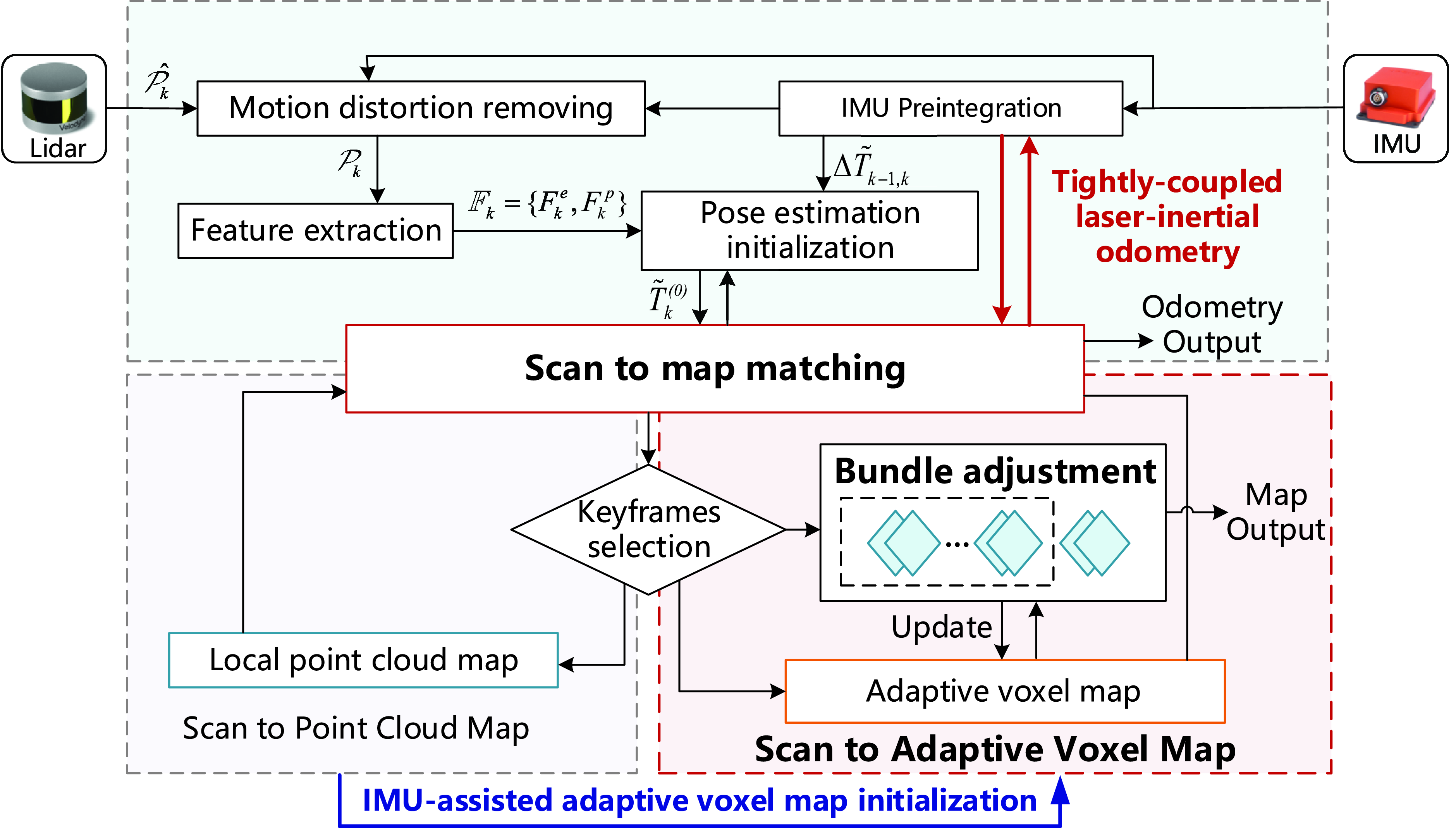
Figure 1. BA-LIOM system overview.
4. Preprocessing of data
In this paper, the world frame and the robot body frame are denoted as W and B, respectively. For ease of depiction, the body frame of robot and the IMU frame are assumed identical (aligned by calibrated external parameters). Then the state of the robot $\boldsymbol{{x}}$
in W is given as
$\boldsymbol{{x}}$
in W is given as
 \begin{equation} x=\left[R^T \quad p^T \quad v^T \quad b^T\right]^T, \end{equation}
where ${\boldsymbol{{R}}}\in SO(3)$
represents the rotation matrix,
${\boldsymbol{{R}}}\in SO(3)$
represents the rotation matrix, ${\boldsymbol{{p}}}\in \mathbb{R}^3$
represents the position vector,
${\boldsymbol{{p}}}\in \mathbb{R}^3$
represents the position vector, ${\boldsymbol{{v}}} \in \mathbb{R}^3$
represents the speed, and
${\boldsymbol{{v}}} \in \mathbb{R}^3$
represents the speed, and ${\boldsymbol{{b}}} = [{{\boldsymbol{{b}}}^g} \quad{\boldsymbol{{b}}}^a]$
represents the IMU bias. The transformation from W to B is denoted by
${\boldsymbol{{b}}} = [{{\boldsymbol{{b}}}^g} \quad{\boldsymbol{{b}}}^a]$
represents the IMU bias. The transformation from W to B is denoted by ${\boldsymbol{{T}}}=\left [{\boldsymbol{{R}}} \mid{\boldsymbol{{p}}} \right ] \in SE(3)$
(i.e.,
${\boldsymbol{{T}}}=\left [{\boldsymbol{{R}}} \mid{\boldsymbol{{p}}} \right ] \in SE(3)$
(i.e., $_{{\boldsymbol{{B}}}}^{{\boldsymbol{{W}}}}{\boldsymbol{{T}}}$
).
$_{{\boldsymbol{{B}}}}^{{\boldsymbol{{W}}}}{\boldsymbol{{T}}}$
).
4.1. Motion distortion removing
Due to the physical rules of the rotating lidar and the motion of the vehicle, motion distortion of the laser point cloud is inevitable. The high frequency and high precision acceleration and velocity measurements from IMU enable the estimation of nonlinear motion within one lidar rotation cycle.
The IMU preintegration method recommended in ref. [Reference Forster, Carlone, Dellaert and Scaramuzza26] is used to calculate the relative body motion between two timesteps. The preintegrated measurements $\Delta \boldsymbol{{v}}_{ij}$
,
$\Delta \boldsymbol{{v}}_{ij}$
, $\Delta{\boldsymbol{{p}}}_{ij}$
, and
$\Delta{\boldsymbol{{p}}}_{ij}$
, and $\Delta{\boldsymbol{{R}}}_{ij}$
between time
$\Delta{\boldsymbol{{R}}}_{ij}$
between time $i$
and
$i$
and $j$
can be calculated by
$j$
can be calculated by
 \begin{equation} \Delta{\boldsymbol{{v}}}_{ij} ={\boldsymbol{{R}}}_i^T \left ({\boldsymbol{{v}}}_j -{\boldsymbol{{v}}}_i -g\Delta t_{ij} \right ), \end{equation}
 \begin{equation} \Delta{\boldsymbol{{p}}}_{ij} ={\boldsymbol{{R}}}_i^T \left ({\boldsymbol{{p}}}_j -{\boldsymbol{{p}}}_i -{\boldsymbol{{v}}}_i \Delta t_{ij} - \frac{1}{2}g\Delta t_{ij}^2 \right ), \end{equation}
 \begin{equation} \Delta{\boldsymbol{{R}}}_{ij} ={\boldsymbol{{R}}}_i^T{\boldsymbol{{R}}}_j. \end{equation}
The point cloud distortion removing makes motion compensation for each point during one scan. The method is to transform the laser points at each moment to the first laser point coordinate system of the lidar scan in which they are located. The rotation increment of each scan is obtained from the integration of the raw IMU data during the scan, and the translation increment is obtained from the IMU odometry.
4.2. Feature extraction
Feature points are needed to be extracted when a new laser scan arrives. The smoothness of points over a local region distinguishes edge and planar points. Largely curved points are considered as edge points; conversely, those with slight curvature are considered as planar points. The rule for evaluating the smoothness of the local surface is defined in ref. [Reference Zhang and Singh27]. The method to obtain stable features is the same as LOAM, which excludes two kinds of points: those on a plane generally parallel to a laser beam and collected under the influence of occluders.
The sets of edge and planar feature points collected from the $k$
th scan are denoted as
$k$
th scan are denoted as $\textrm{F}_k^e$
and
$\textrm{F}_k^e$
and $\textrm{F}_k^p$
, respectively, which constitute the lidar frame
$\textrm{F}_k^p$
, respectively, which constitute the lidar frame $\mathbb{F}_k=\left\{\textrm{F}_k^e,\textrm{F}_k^p\right\}$
represented in B.
$\mathbb{F}_k=\left\{\textrm{F}_k^e,\textrm{F}_k^p\right\}$
represented in B.
4.3. Keyframes selection
BA-LIOM adopts the lidar keyframe strategy to save computing power and increase efficiency. In the area of visual SLAM, the keyframe notion is frequently used. A practical heuristic technique established by spatial transformation is used to choose the current $\mathbb{F}_{k+1}$
as a keyframe when the pose changes over a certain threshold while comparing with the former keyframe
$\mathbb{F}_{k+1}$
as a keyframe when the pose changes over a certain threshold while comparing with the former keyframe $\mathbb{F}_k$
. Specifically, in our outdoor experiments, the current frame is designated as a keyframe if the relative distance change from the previous keyframe is greater than 1
$\mathbb{F}_k$
. Specifically, in our outdoor experiments, the current frame is designated as a keyframe if the relative distance change from the previous keyframe is greater than 1 $\textrm{m}$
or if the orientation changing is greater than 0.2
$\textrm{m}$
or if the orientation changing is greater than 0.2 $^{\circ }$
along any axis. Only keyframes are sent to the BA optimization thread for processing. This method of adding keyframes makes a compromise between memory usage and map density, facilitating real-time optimization.
$^{\circ }$
along any axis. Only keyframes are sent to the BA optimization thread for processing. This method of adding keyframes makes a compromise between memory usage and map density, facilitating real-time optimization.
5. IMU-assisted adaptive voxel map initialization and construction
For efficient feature searching and matching [Reference Ferrer28], an adaptive voxelization method is utilized, which is a relatively sparse representation of environmental features. Compared with traditional point cloud map, the adaptive voxel maps constructed in this study discretize 3D space into voxels and encodes spatial features at the voxel level. Each feature is characterized by its centroid and the associated normal vector or directional vector, constituting a sparse representation of spatial structural information. When environmental information is insufficient during the initial stage, relying solely on point cloud registration for initializing the adaptive voxel map is unreliable. So an IMU-assisted adaptive voxel map initialization and construction approach is proposed to facilitate accurate and robust scan matching and localization, particularly in scenarios involving rapid motion and limited feature availability.
5.1. IMU-assisted adaptive voxel map initialization
The initiation of the adaptive voxel map plays a crucial role in reducing system uncertainty. It is necessary to carefully address the errors that emerge in the initial phase, as they have a propensity to accumulate over time, ultimately impacting the overall localization performance. At the beginning of the procedure, as not enough scans have been received for subsequent BA optimization, a new scan is matched with a local map made up of keyframes in a sliding window. Specifically, a set of the $n$
most recently received keyframes
$n$
most recently received keyframes $\{ \mathbb{F}_{k-n},\ldots,\mathbb{F}_k \}$
is registered into frame W by
$\{ \mathbb{F}_{k-n},\ldots,\mathbb{F}_k \}$
is registered into frame W by $\left\{ \tilde{{\boldsymbol{{T}}} }_{k-n}^{(0)},\ldots,\tilde{{\boldsymbol{{T}}} }_{k}^{(0)} \right\}$
that are associated with them. They are then combined to form a submap
$\left\{ \tilde{{\boldsymbol{{T}}} }_{k-n}^{(0)},\ldots,\tilde{{\boldsymbol{{T}}} }_{k}^{(0)} \right\}$
that are associated with them. They are then combined to form a submap $\textrm{M}_k$
, which is made up of two sub-voxel maps
$\textrm{M}_k$
, which is made up of two sub-voxel maps $\textrm{M}_k^e$
and
$\textrm{M}_k^e$
and $\textrm{M}_k^p$
corresponding to edge and planar feature voxel maps, respectively, that is,
$\textrm{M}_k^p$
corresponding to edge and planar feature voxel maps, respectively, that is, $\textrm{M}_k=\left\{ \textrm{M}_k^e,\textrm{M}_k^p \right\}$
. In order to remove the duplicate feature points that fall within the same voxel,
$\textrm{M}_k=\left\{ \textrm{M}_k^e,\textrm{M}_k^p \right\}$
. In order to remove the duplicate feature points that fall within the same voxel, $\textrm{M}_k^e$
and
$\textrm{M}_k^e$
and $\textrm{M}_k^p$
are downsampled.
$\textrm{M}_k^p$
are downsampled.
During the adaptive voxel map initialization stage, a newly received lidar frame $\mathbb{F}_{k+1}=\left\{ \textrm{F}_{k+1}^e,\textrm{F}_{k+1}^p \right\}$
is matched to
$\mathbb{F}_{k+1}=\left\{ \textrm{F}_{k+1}^e,\textrm{F}_{k+1}^p \right\}$
is matched to $\textrm{M}_k$
via scan matching. The scan matching to local point cloud is the same as ref. [Reference Zhang and Singh27].
$\textrm{M}_k$
via scan matching. The scan matching to local point cloud is the same as ref. [Reference Zhang and Singh27]. $\mathbb{F}_{k+1}$
is transformed from B to W by
$\mathbb{F}_{k+1}$
is transformed from B to W by $\tilde{{\boldsymbol{{T}}}}_{k+1}^{(0)}$
to obtain
$\tilde{{\boldsymbol{{T}}}}_{k+1}^{(0)}$
to obtain $^{\prime}\mathbb{F}_{k+1}=\left\{ ^{\prime}\textrm{F}_{k+1}^e,^{\prime}\textrm{F}_{k+1}^p \right\}$
, where
$^{\prime}\mathbb{F}_{k+1}=\left\{ ^{\prime}\textrm{F}_{k+1}^e,^{\prime}\textrm{F}_{k+1}^p \right\}$
, where $\tilde{{\boldsymbol{{T}}}}_{k+1}^{(0)}=\tilde{{\boldsymbol{{T}}}}_k \Delta \tilde{{\boldsymbol{{T}}}}_{k,k+1}$
,
$\tilde{{\boldsymbol{{T}}}}_{k+1}^{(0)}=\tilde{{\boldsymbol{{T}}}}_k \Delta \tilde{{\boldsymbol{{T}}}}_{k,k+1}$
, $\tilde{{\boldsymbol{{T}}}}_k$
stands for the odometry estimation of the previous frame
$\tilde{{\boldsymbol{{T}}}}_k$
stands for the odometry estimation of the previous frame $\mathbb{F}_k$
.
$\mathbb{F}_k$
. $\Delta \tilde{{\boldsymbol{{T}}}}_{k,k+1}$
denotes the increment prediction during the
$\Delta \tilde{{\boldsymbol{{T}}}}_{k,k+1}$
denotes the increment prediction during the $k$
th scan acquired by the IMU odometry. The motion constraints provided by the IMU effectively compensate for the lack of feature information during the adaptive voxel map initialization phase. It can aid in the precise point cloud registration and accelerates the convergence speed of the optimization. The detailed definition of
$k$
th scan acquired by the IMU odometry. The motion constraints provided by the IMU effectively compensate for the lack of feature information during the adaptive voxel map initialization phase. It can aid in the precise point cloud registration and accelerates the convergence speed of the optimization. The detailed definition of ${\boldsymbol{{d}}}_{e_k}$
and
${\boldsymbol{{d}}}_{e_k}$
and ${\boldsymbol{{d}}}_{p_k}$
is given in ref. [Reference Zhang and Singh27], which indicates the distance between feature point and its corresponding feature in
${\boldsymbol{{d}}}_{p_k}$
is given in ref. [Reference Zhang and Singh27], which indicates the distance between feature point and its corresponding feature in $\textrm{M}_k$
. The optimization issue is formulated as the minimization of the sum of distance residuals.
$\textrm{M}_k$
. The optimization issue is formulated as the minimization of the sum of distance residuals.
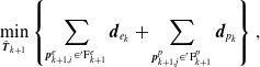 \begin{equation} \mathop{\min }_{\tilde{{\boldsymbol{{T}}}}_{k+1}} \left \{ \sum \limits _{{\boldsymbol{{p}}}_{k+1,i}^e \in ^{\prime}\textrm{F}_{k+1}^e }{\boldsymbol{{d}}}_{e_k} + \sum \limits _{{\boldsymbol{{p}}}_{k+1,j}^p \in ^{\prime}\textrm{F}_{k+1}^p }{\boldsymbol{{d}}}_{p_k} \right \}, \end{equation}
where $i$
and
$i$
and $j$
represent the index of the point in the set to which it belongs. The optimal problem is solved by applying the GaussNewton method.
$j$
represent the index of the point in the set to which it belongs. The optimal problem is solved by applying the GaussNewton method.
The IMU-assisted adaptive voxel map initialization approach can effectively solve the failure and degradation of the adaptive voxel map due to insufficient environmental information at the early stage, which can increase the system’s adaptability and robustness.
5.2. IMU-assisted construction of the adaptive voxel map
Consider a collection of feature points $\left\{{\boldsymbol{{p}}}_{f_1},{\boldsymbol{{p}}}_{f_2},\ldots,{\boldsymbol{{p}}}_{f_N} \right\}$
drawn from
$\left\{{\boldsymbol{{p}}}_{f_1},{\boldsymbol{{p}}}_{f_2},\ldots,{\boldsymbol{{p}}}_{f_N} \right\}$
drawn from $M$
keyframes and indicate the same edge or plane feature, where
$M$
keyframes and indicate the same edge or plane feature, where ${\boldsymbol{{p}}}_{f_i}$
belongs to the
${\boldsymbol{{p}}}_{f_i}$
belongs to the $s_i$
-th scan. The feature points are transformed from
$s_i$
-th scan. The feature points are transformed from $\textbf{B}$
to
$\textbf{B}$
to $\textbf{W}$
by the pose estimation from scan matching
$\textbf{W}$
by the pose estimation from scan matching $\tilde{{\boldsymbol{{T}}} }_{s_i}$
, where
$\tilde{{\boldsymbol{{T}}} }_{s_i}$
, where $\tilde{{\boldsymbol{{T}}} }_{s_i}=\big[ \tilde{{\boldsymbol{{R}}}}_{s_i} | \tilde{{\boldsymbol{{t}}}}_{s_i} \big] \in SE(3)$
:
$\tilde{{\boldsymbol{{T}}} }_{s_i}=\big[ \tilde{{\boldsymbol{{R}}}}_{s_i} | \tilde{{\boldsymbol{{t}}}}_{s_i} \big] \in SE(3)$
:
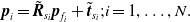 \begin{equation} {\boldsymbol{{p}}}_i=\tilde{{\boldsymbol{{R}}} }_{s_i}{\boldsymbol{{p}}}_{f_i}+\tilde{{\boldsymbol{{t}}}}_{s_i};i=1,\ldots,N. \end{equation}
The center $\bar{{\boldsymbol{{p}}}}$
and covariance matrix
$\bar{{\boldsymbol{{p}}}}$
and covariance matrix $\boldsymbol{{A}}$
for these points are
$\boldsymbol{{A}}$
for these points are
 \begin{equation} \bar{{\boldsymbol{{p}}}}=\frac{1}{N}\sum \limits _{i=1}^N{\boldsymbol{{p}}}_i;\ {\boldsymbol{{A}}}=\frac{1}{N}\sum \limits _{i=1}^N ({\boldsymbol{{p}}}_i-\bar{{\boldsymbol{{p}}}})({\boldsymbol{{p}}}_i-\bar{{\boldsymbol{{p}}}})^T. \end{equation}
The $k$
th largest eigenvalue and the associated eigenvector of matrix
$k$
th largest eigenvalue and the associated eigenvector of matrix $\boldsymbol{{A}}$
is denoted by
$\boldsymbol{{A}}$
is denoted by $\lambda _k({\boldsymbol{{A}}})$
and
$\lambda _k({\boldsymbol{{A}}})$
and ${\boldsymbol{{u}}}_k$
.
${\boldsymbol{{u}}}_k$
.
As shown in Fig. 1, all points in the received keyframes are converted into the global coordinate system in the above manner. Afterward, the 3D space is repeatedly voxelized from a default size (1 $\textrm{m}$
). Eigenvalues and eigenvectors of
$\textrm{m}$
). Eigenvalues and eigenvectors of $\boldsymbol{{A}}$
in (7) are used to determine whether feature points in a voxel are located on a certain feature. An edge (or a plane) feature is represented by
$\boldsymbol{{A}}$
in (7) are used to determine whether feature points in a voxel are located on a certain feature. An edge (or a plane) feature is represented by $\bar{{\boldsymbol{{p}}}}$
and a unit vector
$\bar{{\boldsymbol{{p}}}}$
and a unit vector $\boldsymbol{{n}}$
.
$\boldsymbol{{n}}$
. $\boldsymbol{{n}}$
characterizes where the geometric feature is oriented, which is the direction vector for edge (i.e.,
$\boldsymbol{{n}}$
characterizes where the geometric feature is oriented, which is the direction vector for edge (i.e., ${\boldsymbol{{u}}}_1$
) and the normal vector for plane (i.e.,
${\boldsymbol{{u}}}_1$
) and the normal vector for plane (i.e., ${\boldsymbol{{u}}}_3$
).
${\boldsymbol{{u}}}_3$
).
An octree structure naturally accommodates the voxel map. To decrease the depth of the octree, a set of octrees are indexed using a hash table. A cube of default size (e.g., 1 $\textrm{m}^3$
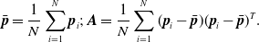
) in space, on which an octree will be constructed if it is not empty. The cube is continuously divided by whether the points in it lie on the same feature, with the result that each leaf node (i.e., a voxel) corresponds to the same geometric feature (i.e., edge or plane) in the 3D space. The process of construction of adaptive voxel map is shown in Algorithm 1.
$\textrm{m}^3$
) in space, on which an octree will be constructed if it is not empty. The cube is continuously divided by whether the points in it lie on the same feature, with the result that each leaf node (i.e., a voxel) corresponds to the same geometric feature (i.e., edge or plane) in the 3D space. The process of construction of adaptive voxel map is shown in Algorithm 1.
Algorithm 1: Construction of adaptive voxel map
This adaptive voxelization method is more effective [Reference Liu and Zhang29], especially for environments with large edges and planes. It can avoid the shortcomings of constructing Kd-tree directly on feature points, which may terminate early when the points all lie in one feature. The adaptive voxel map shown in Fig. 2 stores and represents the geometry in 3D space and can facilitate efficient feature searching and alignment.
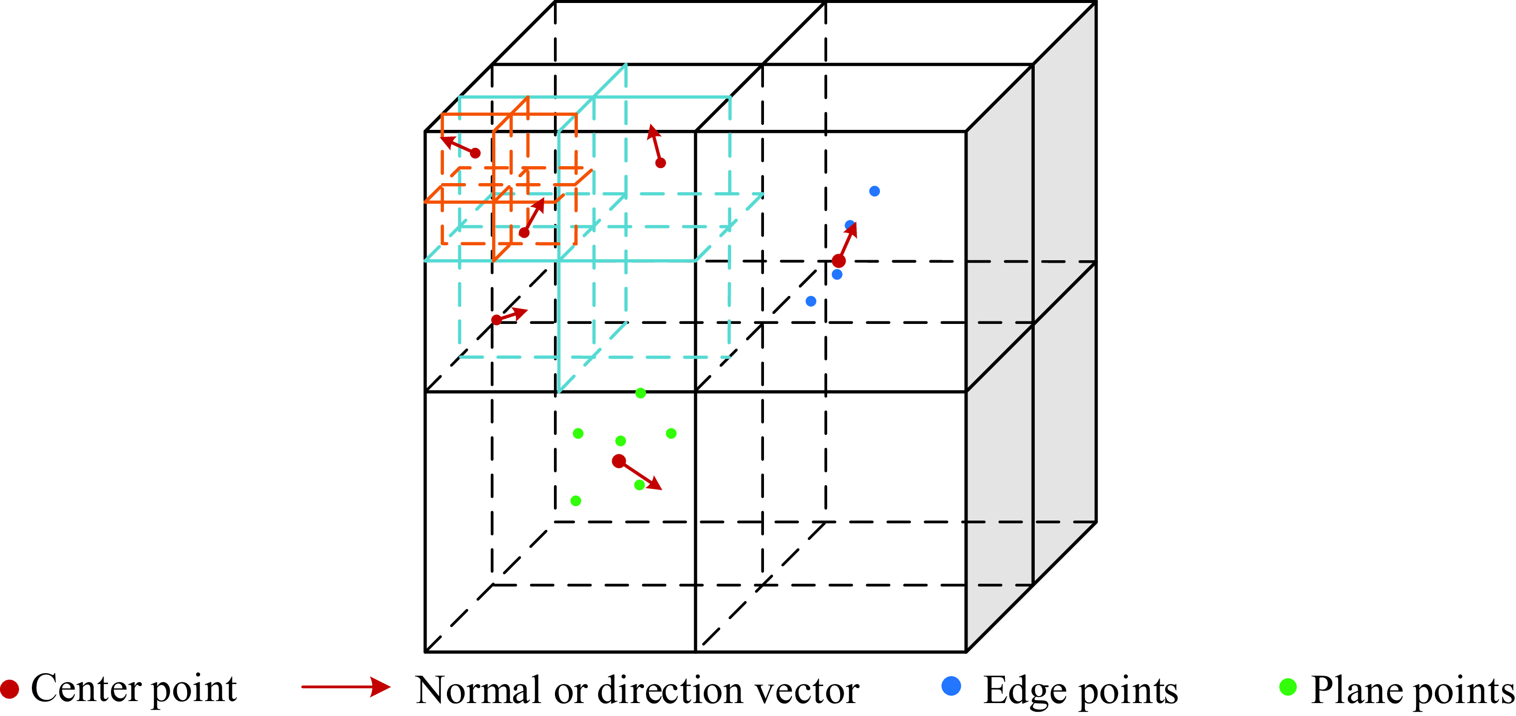
Figure 2. Voxel map.
6. Scanmatching and tightlycoupled odometry on adaptive voxel map
6.1. Tightly-coupled odometry
Assuming that the adaptive voxel maps have been successfully initialized, the new keyframe $\mathbb{F}_{k+1}=\left\{\textrm{F}_{k+1}^e,\textrm{F}_{k+1}^p\right\}$
is matched with the adaptive voxel map
$\mathbb{F}_{k+1}=\left\{\textrm{F}_{k+1}^e,\textrm{F}_{k+1}^p\right\}$
is matched with the adaptive voxel map $^{\prime}\textrm{M}_k=\left\{ ^{\prime}\textrm{M}_k^e,^{\prime}\textrm{M}_k^p \right\}$
. The same as Section 5.1,
$^{\prime}\textrm{M}_k=\left\{ ^{\prime}\textrm{M}_k^e,^{\prime}\textrm{M}_k^p \right\}$
. The same as Section 5.1, $\mathbb{F}_{k+1}$
is transformed to W by
$\mathbb{F}_{k+1}$
is transformed to W by $\tilde{{\boldsymbol{{T}}} }_{k+1}^{(0)}$
and then
$\tilde{{\boldsymbol{{T}}} }_{k+1}^{(0)}$
and then $^{\prime}\mathbb{F}_{k+1}=\left\{ ^{\prime}\textrm{F}_{k+1}^e,^{\prime}\textrm{F}_{k+1}^p \right\}$
is obtained. More specifically, for each point in
$^{\prime}\mathbb{F}_{k+1}=\left\{ ^{\prime}\textrm{F}_{k+1}^e,^{\prime}\textrm{F}_{k+1}^p \right\}$
is obtained. More specifically, for each point in $^{\prime}\mathbb{F}_{k+1}$
, despite fitting its correspondence feature by least squares, we search for the nearest voxel represented by
$^{\prime}\mathbb{F}_{k+1}$
, despite fitting its correspondence feature by least squares, we search for the nearest voxel represented by $\bar{{\boldsymbol{{p}}}}$
and
$\bar{{\boldsymbol{{p}}}}$
and $\boldsymbol{{n}}$
based on distance. The simplification leads to speeding up of matching process.
$\boldsymbol{{n}}$
based on distance. The simplification leads to speeding up of matching process.
The factor graph on which the tightly coupled odometry is built is depicted in Fig. 3. The pose estimation acquired by scan matching to adaptive voxel map is added to a factor graph as lidar odometry factor. The IMU preintegration factor between two adjacent keyframes is added for constraining the pose, velocity, and bias. The proposed method tightly couples the estimation of lidar with the IMU state variables and updates the pose and velocity estimates and IMU bias in real time. This operation fully accounts for the inherent constraints of lidar and IMU observations, which can significantly increase the accuracy of the framework and enhance noise inclusiveness. Therefore, BA-LIOM can achieve excellent performance in some scenarios with fast motion or lack of structural features.
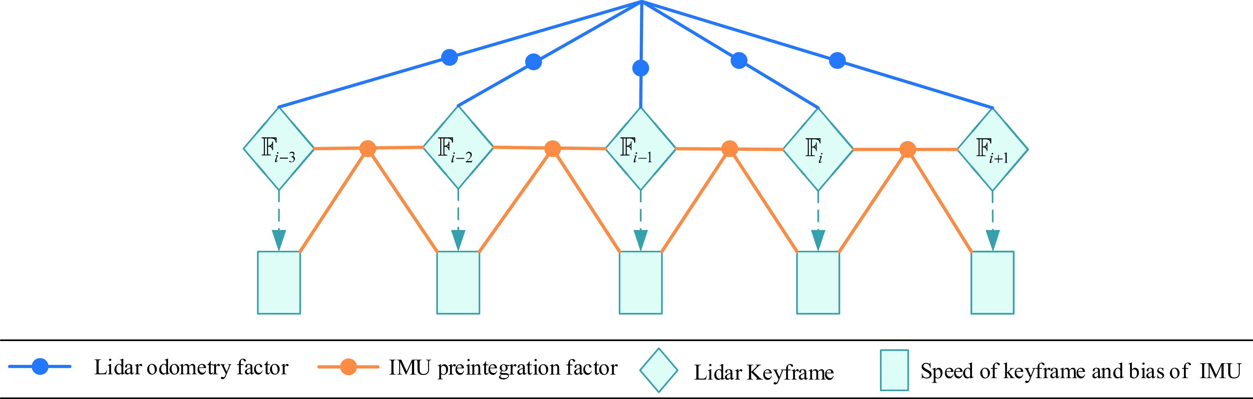
Figure 3. Factor graph of the tightly coupled odometry.
6.2. Scan matching on adaptive voxel map
The BA on lidar frames is similar to the multiview registration in the visual SLAM field. Unlike those methods which build the map incrementally [Reference Shan and Englot12, Reference Zhang and Singh27, Reference Lin and Zhang30], this paper performs local lidar BA on a sliding window of lidar keyframes. By using concurrency constraints from multiple frames, information from recent scans can be used to reevaluate the past scans. The pose estimation of all scans in the sliding window can be adjusted for regional temporal and spatial correlations. Due to the sparsity of feature points, it is challenging to conduct BA on lidar frames. The lidar BA in this paper is formulated as minimizing the distance between a feature point and its corresponding edge or plane, as shown in Fig. 4. The detailed derivation and formulation of the efficient lidar BA are given in ref. [Reference Liu and Zhang29]. Due to the characteristics of the adaptive voxel map, plane or edge features are stored at the voxel level. Each feature is represented by its centroid and the associated normal vector or directional vector. For establishing correspondences, we only need to search for the nearest centroids and then calculate the distance from the point to its corresponding feature. The distance residual is used as the loss function in optimization to obtain the final matching result.
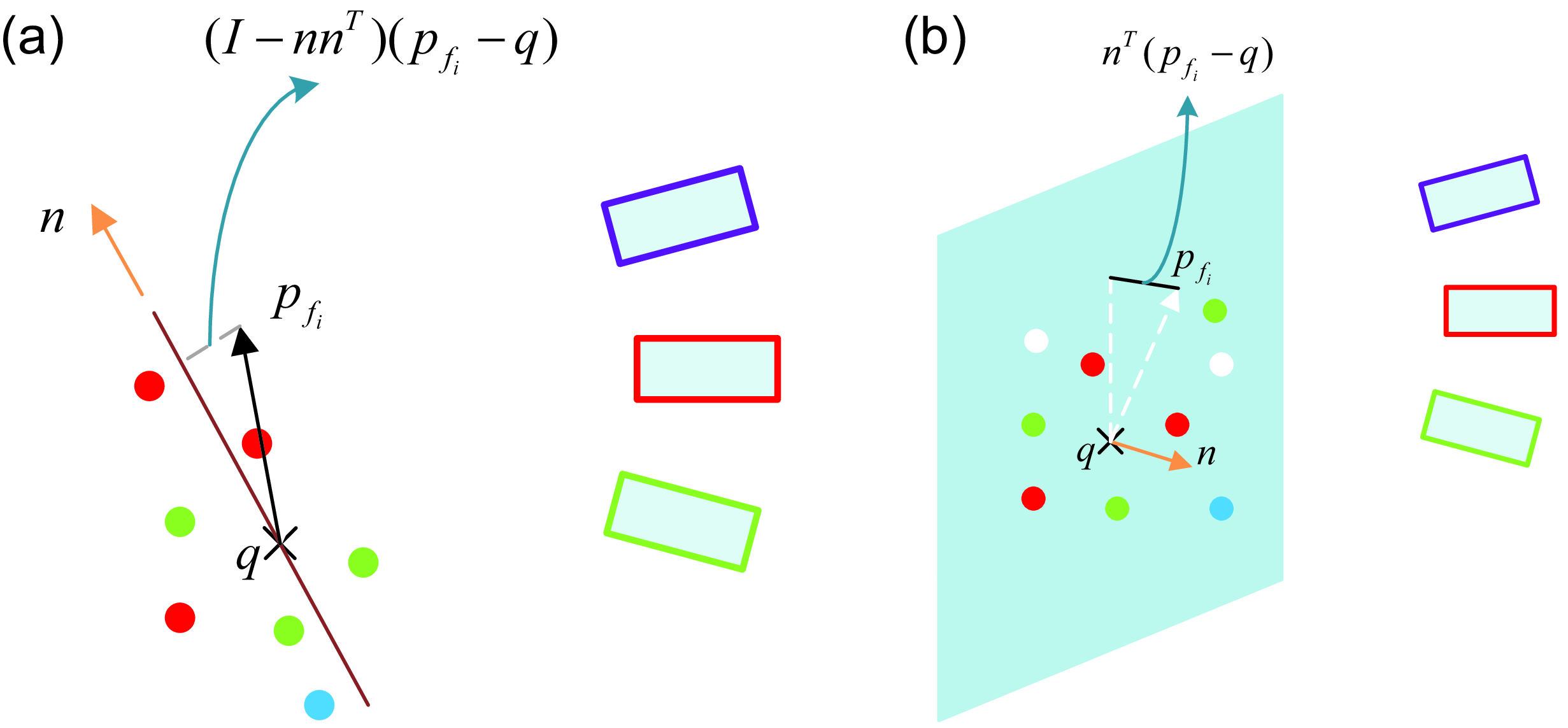
Figure 4. Feature and the corresponding feature points drawn from multiple keyframes: (a) Edge feature. (b) Plane feature.
7. Experiment
Experiments have conducted to analyze the performance of BA-LIOM qualitatively and quantitatively. The mobile platform is equipped with a Velodyne VLP-16 lidar, an Xsense MTi-300 IMU, and a CHC CGI-610 integrated navigation system, where the GPS-RTK measurements are used as ground truth. The sensors have realized hardware trigger and time synchronization based on pulse per second (PPS) and National Marine Electronics Association (NEMA) of CGI-610. The experimental platform and sensors are shown in Fig. 5(a).
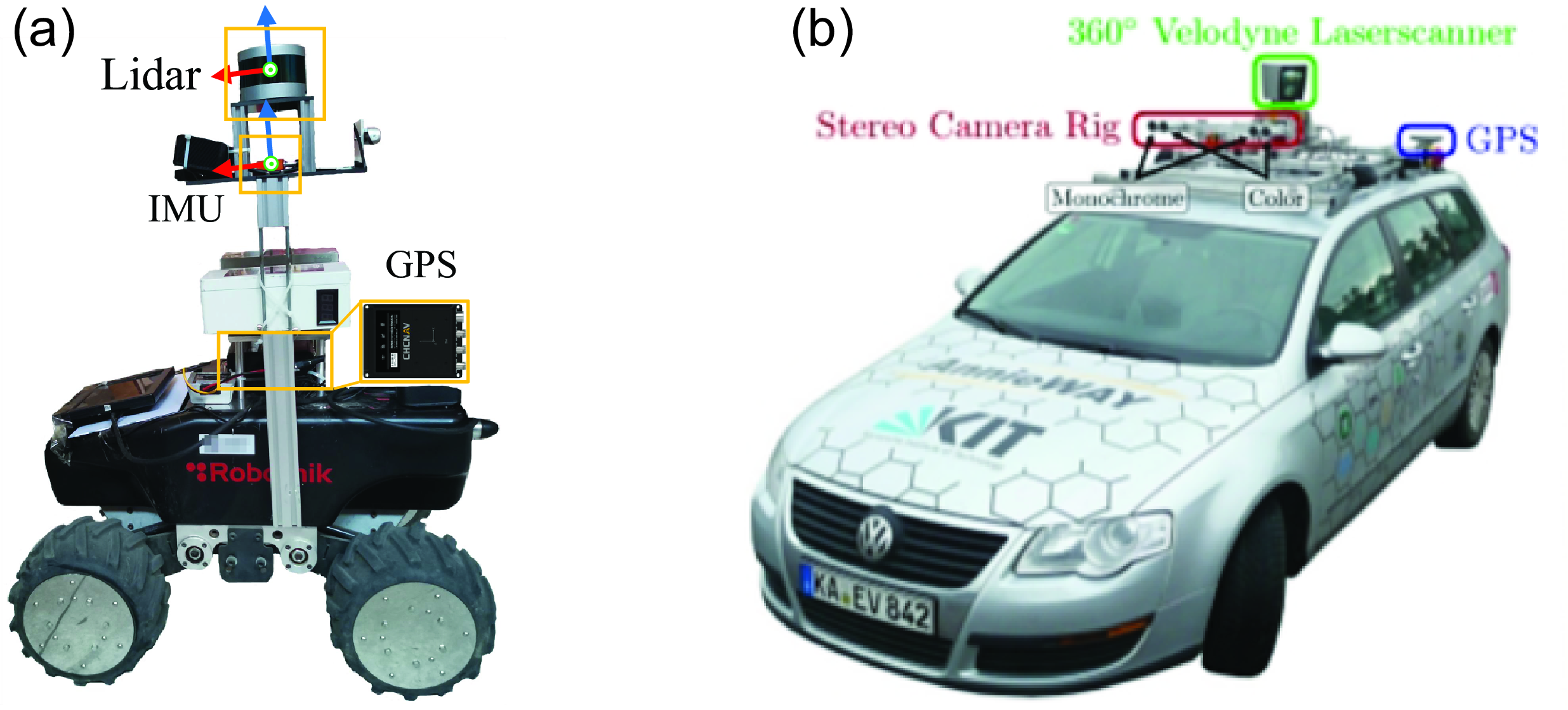
Figure 5. Platforms for data collection: (a) Self-assembled platform. The self-assembled sensors have done hardware synchronization and parameters calibration. (b) Sensor configuration and vehicle used by the KITTI benchmark. The station is equipped with cameras, a Velodyne HDL-64E laser scanner and a GPS localization system.
To validate the widespread feasibility of BA-LIOM, we conducted extensive experimental validation on self-record and public datasets. We collect four different datasets across various scales and environments using our self-assembled platform shown in Fig. 5(a), which are referred to as buildings, square, lawn, and grove, respectively. What is more, BA-LIOM has also been evaluated on the dataset from the KITTI odometry benchmark, and the platform used is shown in Fig. 5(b).
The proposed framework has been compared with LOAM, BALM, and LIO-SAM. In the experiments, the algorithms are all forced to run in real time on a laptop computer with Intel Core i7-10870H 2.20 GHz, 16G RAM. The software platform is Ubuntu 18.04 with ROS melodic software framework. All of the methods are implemented in C++.
7.1. Buildings dataset
The dataset is recorded by manipulating the unmanned ground vehicle around the college for simulating the urban road environment. The experiment aims to assess the performance of BA-LIOM in dealing with the translation and rotation of the vehicle, besides the trajectory drift and localization errors while running for a long time. The test environment and mapping result are shown in Fig. 6.
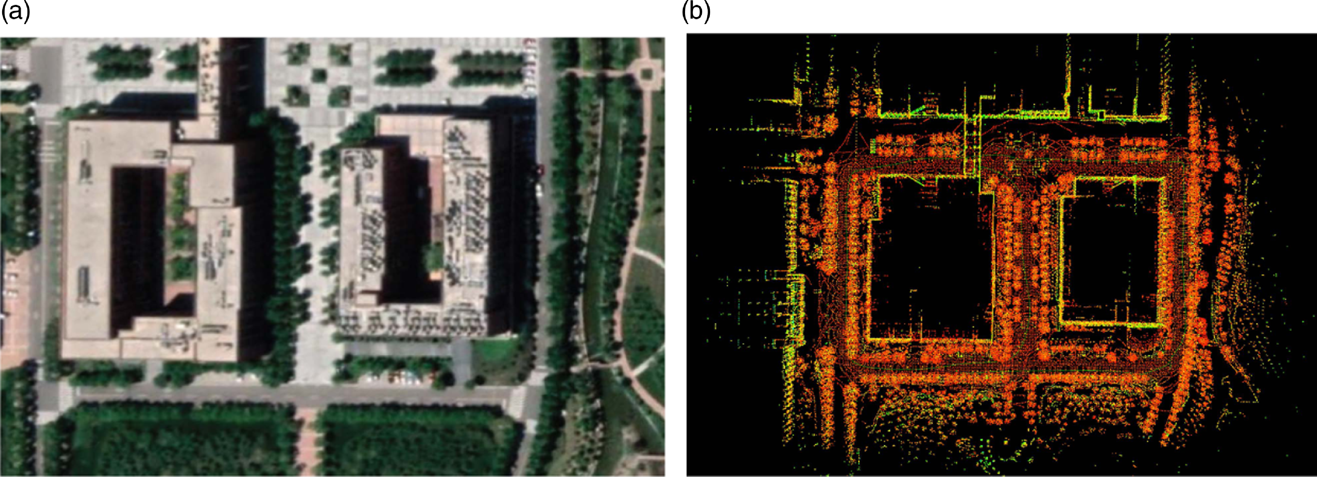
Figure 6. Environment and mapping result of BA-LIOM in the buildings. (a) Test environment. (b) Google map. (c) Mapping result of BA-LIOM.
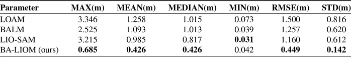
The trajectories and evaluation results of LOAM, BALM, and LIO-SAM and are shown in Fig. 7. The output trajectories of the above methods and the ground truth are shown in Fig. 7(a). The XYZ directional components of the trajectories in a global coordinate system are shown in Fig. 7(b). The outputs of the four methods show no obvious deviation in the horizontal direction, while there is a noticeable variance in the height. It can be seen that the trajectory of BA-LIOM almost coincide with the ground truth, LIO-SAM has a slight deviation, and the trajectories of BALM and LOAM deviate from the ground truth and accumulate with time. The absolute errors of the trajectories are evaluated quantitatively, as shown in Table I, in which the optimal results are thickened. Among the statistical indicators, except that the minimum value of BA-LIOM is slightly higher than that of LIO-SAM, the other indicators are better than the other three methods. The root mean square error (RMSE) of BA-LIOM is decreased by 61–70% compared with others, and the standard deviation (STD) is reduced by 76–83%. Overall, the proposed framework has the smallest trajectory error and the highest robustness.
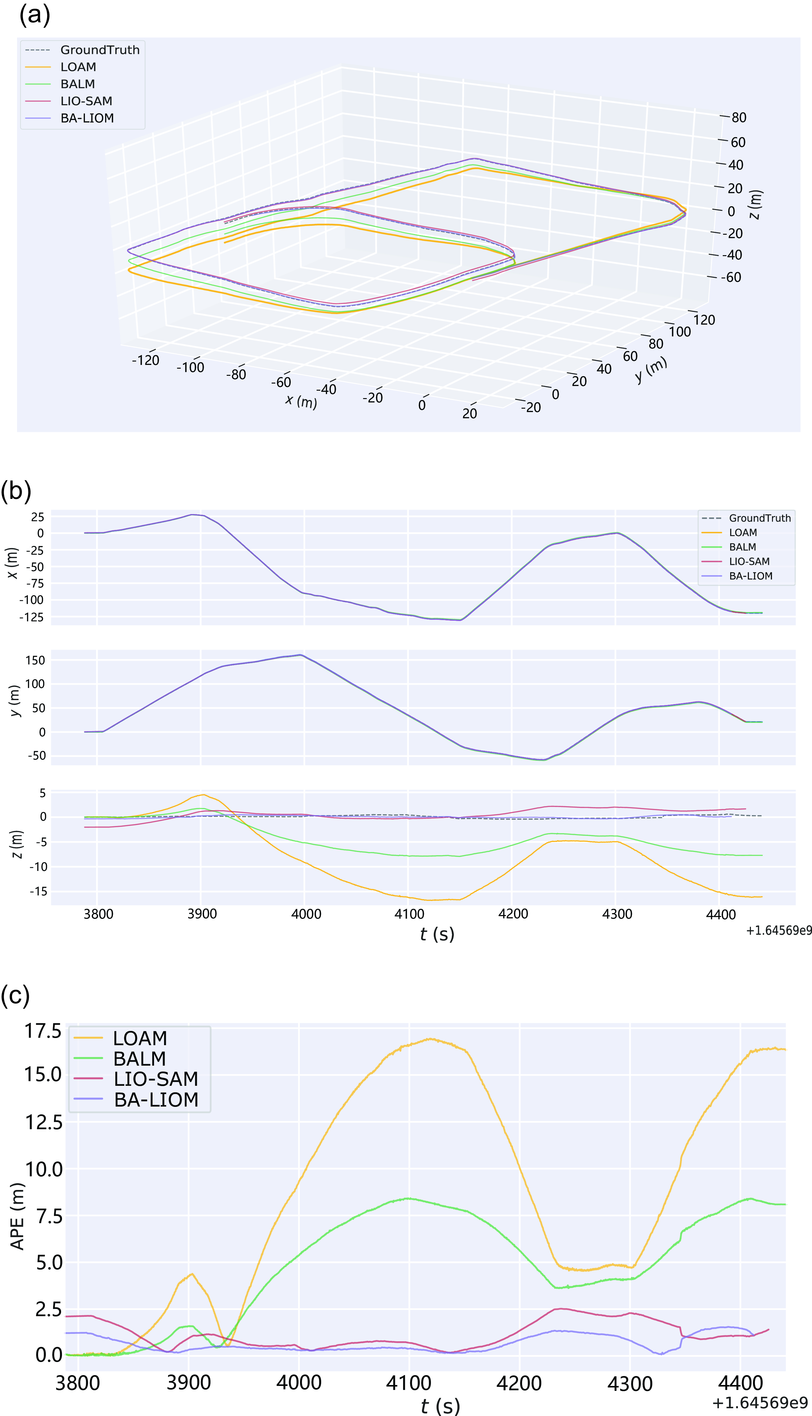
Figure 7. Comparison and evaluation results of LOAM, BALM, LIO-SAM, and BA-LIOM (ours). (a) Trajectory. (b) XYZ directional trajectory component. (c) Absolute pose error of trajectories.
Table I. Buildings dataset: absolute trajectory error.
7.2. Square dataset
The dataset was recorded around a small library in the middle of the square and returned to its starting position at the end of the trajectory. The trajectory is shorter than that of the buildings dataset. But the platform will pass through the slightly bumpy masonry road, which will cause a certain degree of disturbance to the sensors carried on the mobile platform, especially the IMU, and bring challenges to the robustness of the algorithm and causing an impact on the localization accuracy. The map of the square and the mapping result is shown in Fig. 8.
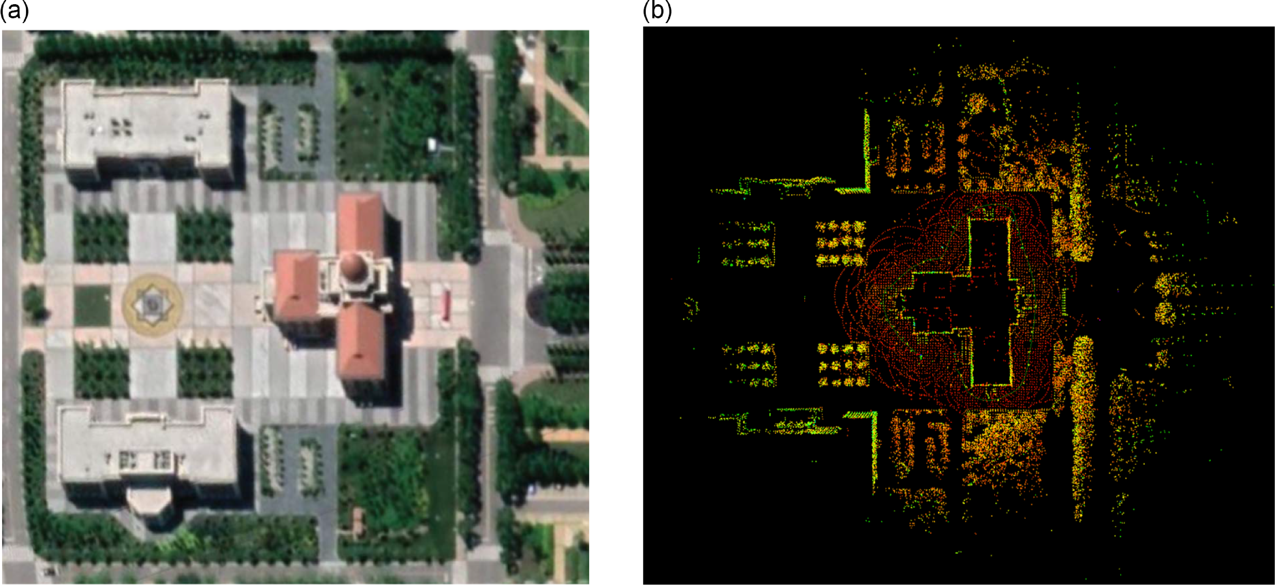
Figure 8. Environment and mapping result of proposed framework in the square. (a) Google map. (b) Mapping result of BA-LIOM.
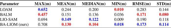
Table II shows the statistical findings of the quantitative analysis of the absolute pose error of the output trajectories relative to the ground truth. The values of red and blue marks represent the minimum and sub-minimum values in the column, respectively. BA-LIOM occupies two best and three second best of the seven evaluation indicators. Generally speaking, the error and robustness of the proposed framework in this scene are better than other comparison methods.
Table II. Square dataset: absolute trajectory error.
7.3. Lawn dataset
This dataset is recorded around a big lawn, which has a long side nearly 400 $\textrm{m}$
. The final location of the verification trajectory coincides with the initial position, allowing for seeing the cumulative drift of BA-LIOM. The environment and mapping result of lawn are shown in Fig. 9.
$\textrm{m}$
. The final location of the verification trajectory coincides with the initial position, allowing for seeing the cumulative drift of BA-LIOM. The environment and mapping result of lawn are shown in Fig. 9.
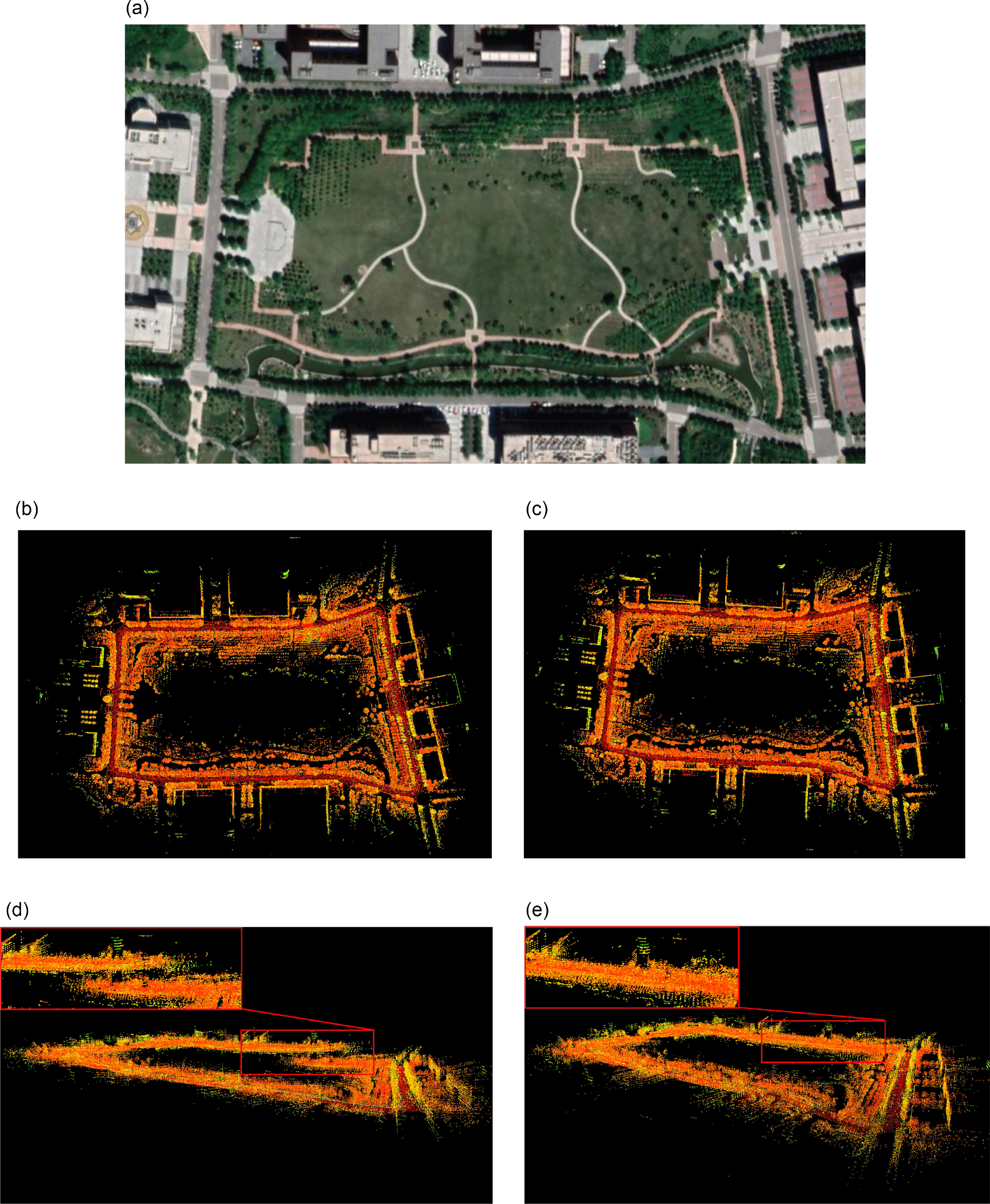
Figure 9. Environment and mapping result in the lawn. (a) Google map. (b)(d) LIO-SAM. (c)(e) Mapping result of BA-LIOM (ours).
The point cloud maps created using the two techniques seem very similar from overhead. However, due to the height drift of LIO-SAM, the map at the end of the trajectory cannot be connected with the starting map. Although there is no auxiliary of the closed-loop detection module, BA-LIOM suppresses the accumulation of drift effectively through local BA. It ensures a great mapping performance when running for a long time.
Figure 10 shows the absolute error curve of LIO-SAM and BA-LIOM relative to the ground truth on lawn. In this scenario, the mean and median of the proposed method are much smaller than that of LIO-SAM. And the RMSE and STD are reduced by $73\%$
and
$73\%$
and $77\%$
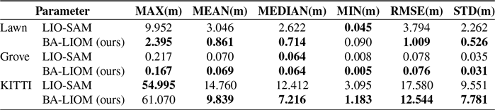
, respectively, compared with LIO-SAM on this dataset. Overall, BA-LIOM can dramatically increase localization accuracy and reduce odometry drift. The quantitative evaluation of the absolute pose error is shown in Table III, in which the optimal value is thickened.
$77\%$
, respectively, compared with LIO-SAM on this dataset. Overall, BA-LIOM can dramatically increase localization accuracy and reduce odometry drift. The quantitative evaluation of the absolute pose error is shown in Table III, in which the optimal value is thickened.
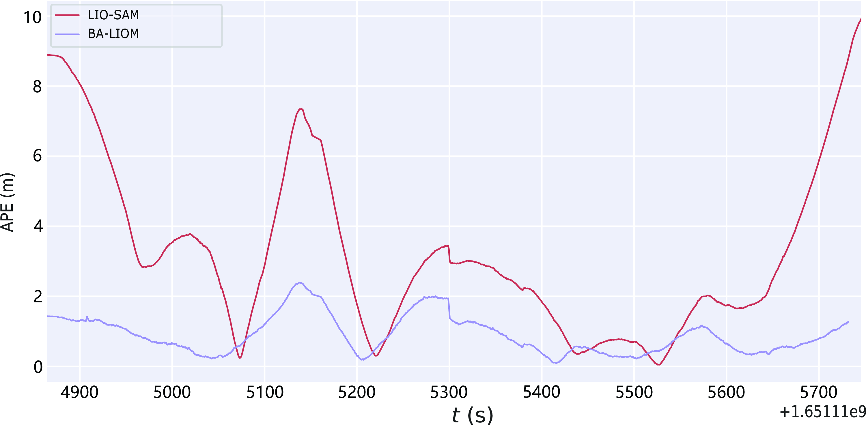
Figure 10. Absolute pose error of LIO-SAM and BA-LIOM (ours).
Table III. Absolute trajectory error.
7.4. Grove dataset
This dataset was recorded in the grove. It is more challenging than buildings. The lack of complete and quality features makes extracting scan-matching difficult. In this case, the fusion of IMU measurements ensures the performance and robustness of the system. BALM failed at the midway through this dataset. Comparing the maps constructed by BALM (before failure interruption) and BA-LIOM, the proposed framework has a much clearer texture of the environment details, as shown in Fig. 11.
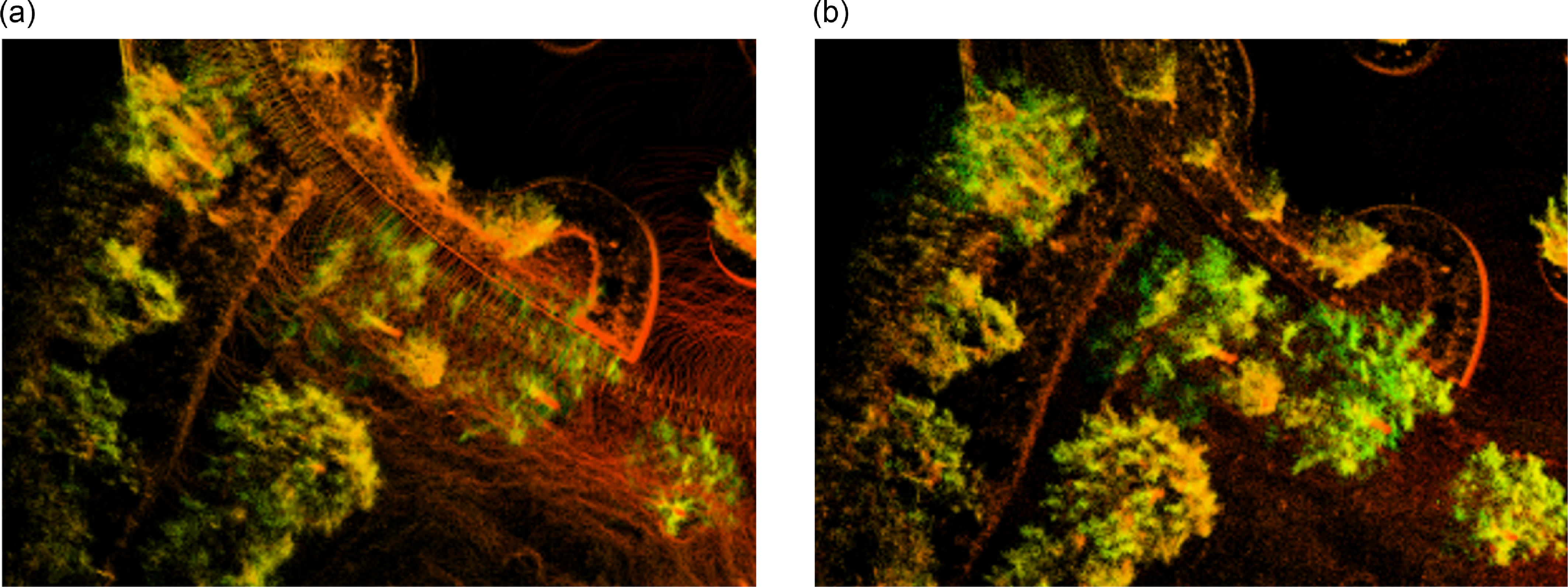
Figure 11. Mapping result of BALM and BA-LIOM in the grove. (a) BALM. (b) BA-LIOM (ours).
7.5. KITTI datasets
KITTI datasets have been widely used for autopilot research and evaluation. The datasets consist of corrected and synchronized images, lidar frames, high-precision GPS, and IMU acceleration information. In this paper, the dataset 2011_09_30_drive_0028 is used to test. The information provided by lidar (VelodyneHDL-64E,10 Hz) and GPS/IMU (OXTS RT3003) are used. To verify the accuracy and effectiveness of BA-LIOM in long-time and large-scale localization and mapping, we compare the experimental result of the proposed process with LIO-SAM.
The mapping result of LIO-SAM and BA-LIOM is shown in Fig. 12. While crossing the same road twice, there is a significant deviation in the trajectory of LIO-SAM. However, in the map constructed by BA-LIOM, the track of the two times passing through this section almost coincides.
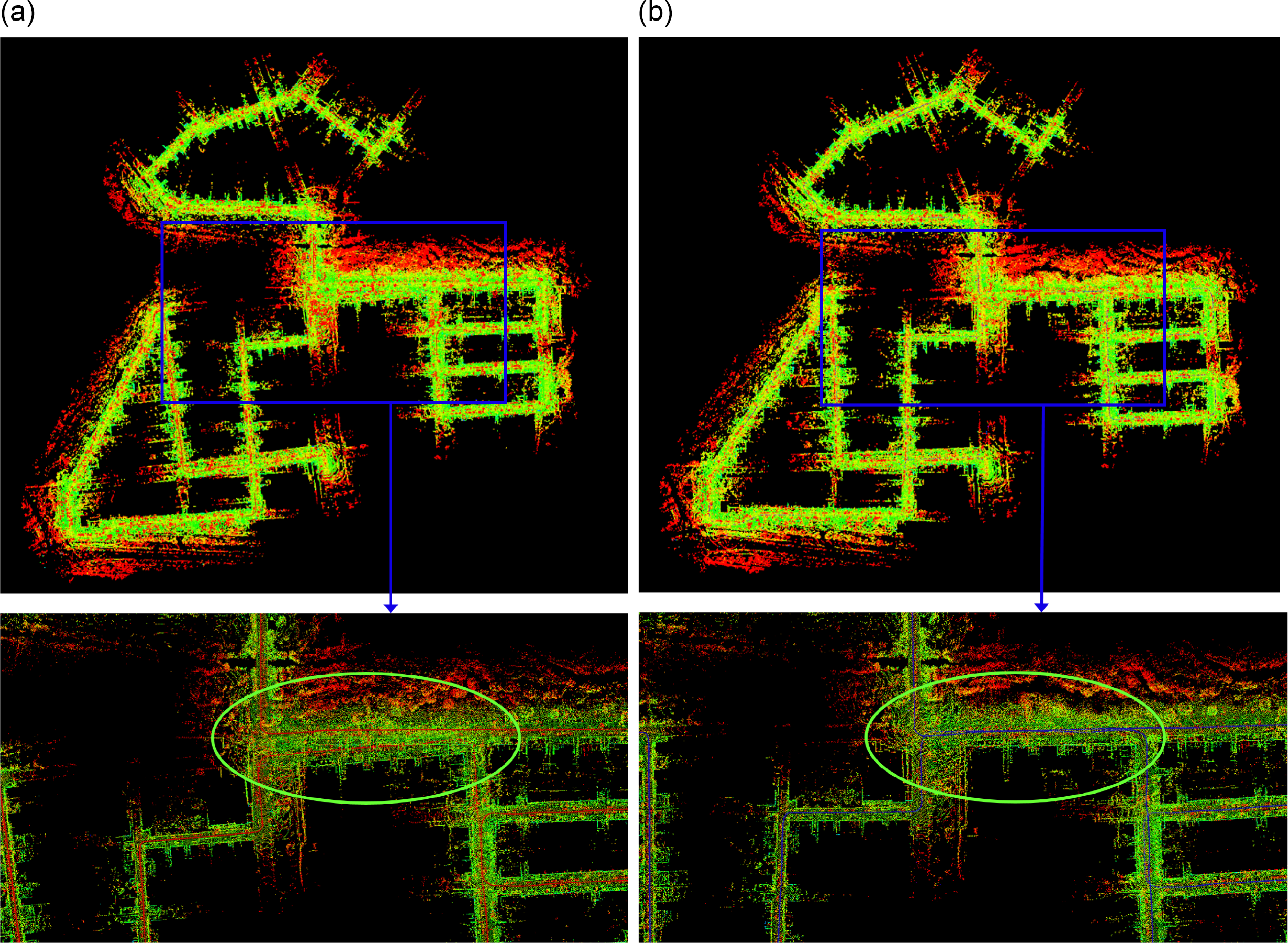
Figure 12. Mapping result of LIO-SAM and BA-LIOM in the KITTI. (a) LIO-SAM. (b) Mapping result of BA-LIOM (ours).
The trajectories of the two methods are displayed in the xy plane as shown in Fig. 13. The output trajectory of BA-LIOM very well matched with the ground truth, while that of LIO-SAM drifts more and more serious over time. Table III displays the findings of the quantitative examination, except that the maximum absolute error index is slightly larger than LIO-SAM, and the other indicators are better than LIO-SAM, especially the MEAN, MEDIAN, and RMSE. When representing the accuracy by RMSE, the accuracy of BA-LIOM is $29\%$
higher than that of LIO-SAM.
$29\%$
higher than that of LIO-SAM.
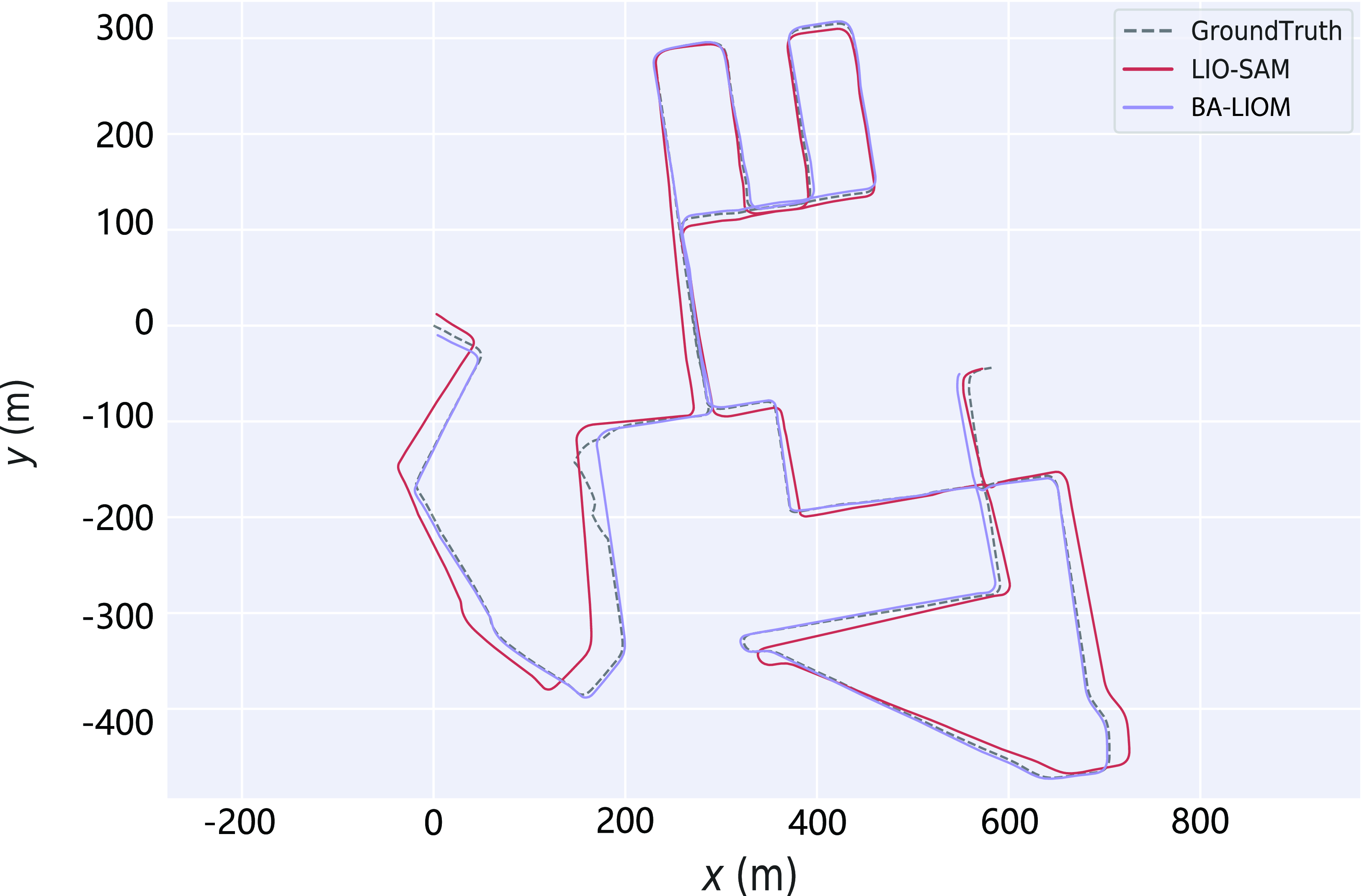
Figure 13. Trajectories of LIO-SAM and BA-LIOM in KITTI dataset.
According to the aforementioned experimental findings, BA-LIOM can significantly increase localization accuracy and successfully reduce cumulative drift when large-scale mapping is conducted over an extended period of time.
8. Conclusions
This paper proposes a framework for laser-inertial odometry and mapping based on map optimization, which can perform in real time and robustly in various scenarios. The system is built atop a factor graph for the fusion of lidar and IMU measurements. Compared to lidar-only odometry, the fusion of IMU allows the framework to be adapted to featureless scenarios and fast movements. The core of this system is a tightly coupled laser-inertial odometry with BA on the back end to optimize the lidar point clouds and keyframe poses as well as the IMU bias in real time. This can considerably decrease the drift of odometry and relieve the issue of ground warping caused by sparse laser scans. Moreover, the BA thread maintains two global voxel maps for edge and plane features, respectively, which consists of optimized points and is constantly updated with BA optimization. The maps make full use of IMU preintegration as priori information and contain a wealth of historical and current environmental information. Because of the correspondence between voxels and features, scan matching can be made efficient at a global level. BA-LIOM is thoroughly evaluated on public and self-record datasets gathered on different platforms across various scenarios. Qualitative and quantitative analysis shows that BA-LIOM can achieve better performance while compared with LIO-SAM and other state-of-art methods. Future work involves improving the robustness of the framework and validating its superiority in more challenging environments.
Author contributions
All authors contributed to the study conception and design. Ruyi Li, Hui Liu, and Songyang Wu conducted data gathering, and Ruyi Li performed data analysis. The first draft of the manuscript was written by Ruyi Li. Xuebo Zhang, Shiyong Zhang, and Jing Yuan provided valuable suggestions on the ideas and manuscript revision.
Financial support
This work was supported in part by the National Natural Science Foundation of China under Grant 62293510 and Grant 62293513, in part by the Tianjin Science Fund for Distinguished Young Scholars under Grant 19JCJQJC62100, and in part by the Fundamental Research Funds for the Central Universities. The author gratefully acknowledges the support of K.C.Wong Education Foundation, Hong Kong.
Competing interests
The authors declare no competing interests exist.
Ethical approval
Not applicable.


