2.1. Vegetation model modification

The fully submerged aquatic plants have little need for stiff or woody tissue as they are able to maintain their position within the water due to their inherent buoyancy, which counteracts their weight (Corker Reference Corker2022). As a result, their cells are usually more flexible than the terrestrial plant cells (Okuda Reference Okuda2002). Therefore, a larger degree of deformation of the aquatic plants is commonly found. Another distinctive feature is that a number of fully submerged plants have finely dissected leaves, which can reduce drag in rivers and provide a larger surface area for photosynthesis and an exchange of minerals and gasses (Sculthorpe Reference Sculthorpe1967). Besides, the leaves are usually arranged radially from the branching points. In other words, there are clusters of finely forked leaves extending from the stem, forming a general spherical shape. While the functions of stems and roots of terrestrial plants are to absorb nutrition from the substrate, for aquatic plants, their main function is anchorage so their shapes are evolved to be relatively thin and soft. Overall, the aforementioned features characterise typical kinds of submerged flexible plants possessing clumped dissected leaves connected by a thin stem and involving a large degree of deformation. Typical examples are Cabomba caroliniana and Ceratophyllum demersum, as shown in figure 1.

Figure 1.

Herbarium photographs of (a) Cabomba caroliniana (scaled), (b) Ceratophyllum demersum (Bugbee et al. Reference Bugbee, Barton, Gibbons and Stebbins2018) and (c) the modified vegetation model used in this study.

In this study, an effective model was developed representing the abovementioned plants, and each plant model was simplified as a series of wooden pellets. Specifically, five pellets (mass density of pellet, ρ_p = 700 kg m⁻³ and pellet diameter, D = 10 ± 0.5 mm) were connected by a fine rope (rope diameter, D_r = 0.3 mm) at 0.02 m interval, which made the plant height h 0.1 m in the still water. Each pellet was disposed by a waterproof material to avoid the large variation of the density during the experiments (Δ ρ_p/ρ_p < 10 %, where Δ ρ_p is the variation of mass density of pellet). This structure was a good representation since all the necessary forces like inertial, buoyance and drag forces, which dominated the mass and momentum interactions with ambient water, were properly dealt with. Compared with the cantilever beams, wall-mounted flexible flaps and plates used in the previous studies, this model manifested a strong three-dimensional nature and a large deformation of the flexible plants, and was convenient to measure the vegetation dynamics. It is worth noting that the restoring force, a force, normally provided by the Young's modulus of the stem for the traditional flexible vegetation, mainly arises from the buoyancy of the densely dissected leaves in this model. Therefore, for simplicity, it was reasonable to use the totally flexible rope as a representation of the highly flexible thin stem for the prototype vegetation, as considered in this study.

With the modified physical model used in the flume, the scientific problem in this study comes down to the dynamics of a string of pellets in an open-channel flow. There are two flow features − a boundary layer flow for a single plant in isolation (figure 2a) and a redirected flow for a vegetation patch of stringed pellets (figure 2b). The pellets of each plant were numbered as one to five from bottom to top for the convenience of description, and each pellet is subject to the gravity, buoyancy and drag induced by the flow and the stress by the strings (figure 2c).

Figure 2.

Idealised sketch of the ‘pellets string’ subject to (a) the open-channel flow, (b) the altered flow and (c) the forces induced to a pellet, where F_buoy is the buoyant force, F_drag is the drag force, F_grav is the gravity force and T_i and T_{i +1} are the inward and outward tensile forces, respectively.

Since the prototype and the model both interacted with the flow of water, the scaling parameters for fluid were unity (λρ_f = λ_μ = λ_g = 1). However, the length scale (λ_l) was set to be 0.2, considering the experimental conditions like flume geometry. Froude similarity was applied here as the situation is similar to the fluid flow applications near a stream boundary in Lambert (Reference Lambert2006), where the gravity effects dominate the viscous forces. Relevant parameters and scaling results are summarised in table 1.

Table 1.

Scaling factors for the system under Froude similarity.

2.2. Experimental apparatus and set-up

Experiments were conducted in a 16 m long, 0.5 m wide and 0.5 m deep glass-wall rectangular flume at the State Key Laboratory of Hydro-Science and Engineering, Tsinghua University, Beijing, as shown in figure 3(a). The slope was adjustable via a lifting gear and was maintained as 0.0025, which is common for alluvial rivers. A flow straightener was installed at the inlet to avoid large-scale motions and swirls in the entry flow. A steady, uniform recirculating flow condition was realised by a centrifugal pump, controlled by a frequency converter through computer, where a linear relationship between frequency and discharge was established. The flow discharge was measured by using an electromagnetic flowmeter fitted on the recirculating pipe. The flow levels were recorded by two water gauges. The measuring section, where a fully developed flow was achieved, was located at 10 m downstream of the flow entrance.

Figure 3.

Schematic views of (a) the experimental flume (not to scale), and two arrangements: (b) plant in isolation (for case S1–S4) and (c) vegetation patch (for case P1–P4). The pellets in red colour are the tracking objects in each experiment.

Considering the redirecting effects of the submerged vegetation patch on the flow, the local flow intensity that the plants within the vegetation patch are subjected to can be quite different from the flow with a plant element in isolation for the same incoming flow. Hence, the swaying characteristics of both the isolated plant in the open-channel flow and the plants in the vegetation patch are investigated. Two sets of arrangements were created in the flume: (i) a single plant model was attached to the flume bottom on the flume axis of symmetry (figure 3b, designated as S), and (ii) a vegetation patch was fabricated with plants mounted at 50 mm intervals extended wall-to-wall spanwise, creating a 1 m long and 0.5 m wide vegetation canopy (figure 3c, designated as P). The vegetation distribution density was 400 stems m⁻², i.e. the solid volume fraction occupied by the plants, φ = 0.0047. The φ value was in accordance with the φ range of marsh grasses (Nepf Reference Nepf2012), but slightly smaller than that of seagrasses. This arrangement allowed measurement of the behaviours of a single plant conveniently. For both the arrangements, the waving dynamics of a single plant was explored, designated as S for a plant in isolation and P for a vegetation patch. The pellets marked in red in figure 3 are the tracking objects in each experiment. All five pellets of a plant were traced to determine their complete behavioural features. The tracer pellets were dyed black with waterproof paint in contrast with the white background.

Four flow discharges (Q = 0.025–0.10 m³ s⁻¹) were run for two arrangements, designated as S1–S4 and P1–P4 for a plant in isolation and a vegetation patch cases, respectively. For the plant in isolation (S1–S4), the plant element was located at the centreline (y = 0) of the spanwise section of the flume. In addition to S1, another set of additional experiments were carried out with the isolated plant at different locations in the spanwise section of the flume, y = 0.25, 0.5, 0.75 and 1.0H, designated as A1–A4. The flow depth H was set as 0.20 m, having a relative submergence (the ratio of flow depth H to plant height h) of 2.0, which was consistent with a shallow relative submergence range of H/h < 5. For a shallow relative submergence, many submerged plants are sustained due to the limited light penetration. Besides, this submergence also fits in with the results of the field survey by the Connecticut Agricultural Experiment Station (Bugbee et al. Reference Bugbee, Barton, Gibbons and Stebbins2018). The flow Reynolds numbers Re (= Q(Bν)^–1, where B is the flume width and ν is the kinematic viscosity of water) ranged 2 × 10⁴–5 × 10⁴ and the flow Froude number Fr (= U_b(gH)^–0.5, where U_b is the area-averaged velocity, i.e. Q(BH)^–1, and g is the gravitational acceleration) varied in the range 0.07–0.18. Experimental conditions are furnished in table 2.

Table 2.

Experimental conditions.

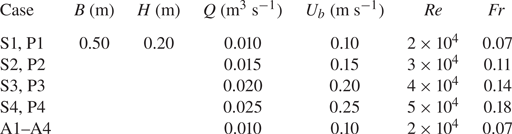
Note: S, P and A are the abbreviations of cases with vegetation in the form of single element, patch and the additional ones.

2.3. Measurement

Three-dimensional velocity statistics were measured by using a down-looking acoustic Doppler velocimeter, named Vectrino, manufactured by Nortek. The sampling duration of Vectrino was 2 min with a rate of 100 Hz and a vertical measuring interval of 20 mm. Due to the limitation of Vectrino, the velocity measurement was not possible 50 mm below the free surface and 10 mm above the bed, thus allowing measurements at eight points across the depth for each sampling position.

The plants’ movements were captured by a Nikon D7200 camera from the top at a frame rate of 30 Hz in 1920 × 1080 pixels. This temporal resolution of image sampling was adequate for capturing a typical pellet oscillation at a frequency of 1–3 Hz. In addition, the spatial resolution was adequate for the detection of pellets’ movement. For each case, the sampling duration of the videos were 10 min, which covered at least 600 typical oscillation periods, and this could be considered to be adequate from a statistical standpoint.

The camera was mounted on the tripod with a 3-way pan-tilt head (Benro, GD3WH), which offered an ideal view for the recording areas and a minimum scale of one degree for adjustment. A calibration plate was shot at different vertical locations for post-calibration of the videos, i.e. different scales apply to five pellets of each plant model when calculating tracks. An extended field depth, or a small enough aperture (the inverse of the f-number, where f is the aperture number of the camera), was set to have a clear sight of all five pellets in the same viewing field. However, it was too small of an aperture to meet the requirement of collecting enough light into the lens, which might subsequently cause an increase in noise in the image. A proper f-number was chosen with a balance between clear and low noise shooting. Moreover, two lamp panels were placed at both the fluid sides to illuminate the shooting area. The experiments were carried out in a dark environment to get the same light for all the cases.

2.4. Data processing

The scaling and lens distortion calibration were carried out before further data processing. The video recording of the swaying motions of the pellets was processed by a MATLAB code using the image processing toolbox. There were three steps to track the pellets’ trajectories. First, the video footage was streamed and cropped into pictures frame by frame, where a later step was performed on each image. Second, the images were transferred to grey, and then the grey scale was stretched, which contained the bottom 1 % and the top 1 % of all pixel values. Median filtering was performed, obtaining the median value in a proper size of neighbourhood of the corresponding pixel. Thereafter, circular Hough transform was applied to find circles in the images, and the proper sensitivity and radius range for the function were set for different cases (Atherton & Kerbyson Reference Atherton and Kerbyson1999). In addition, a property detecting function ‘regionprops’ was employed to verify the results from the abovementioned detection, including the properties, bounding box, centroid and circularity.

The key challenge of the detection was whether one pellet was partly or completely overlapped by a surrounding pellet. Such situation could appear in two flow conditions. For the small discharge (Q = 0.010 m³ s⁻¹), the pellets of a plant were partly overlapped with each other, as shown in figure 4(a). They could be individually detected by setting a higher sensitivity for the circular Hough transform accumulator array, as shown in figure 4(b). On the other hand, for the large discharge (Q = 0.025 m³ s⁻¹), the bottom pellet might be shaded by a top pellet of the neighbouring plant in the upstream direction. When the bottom pellet was half shaded, as shown in figure 4(c), the image dilation method was applied to the picture before further detection (Gonzalez, Woods & Eddins Reference Gonzalez, Woods and Eddins2011). However, in some occasional cases where the bottom pellet was mostly or completely shaded, which was difficult to detect, the position of the shaded pellet could be linearly interpolated by the neighbouring two instances of the same pellet following the time sequence.

Figure 4.

Raw and posted instantaneous images showing the pellets and the detection results. (a) Raw image showing the overlapping of pellets for a small discharge, (b) the posted and detection result of (a), and (c) the top pellet partly shaded by the upstream plant for a large discharge.

For the velocity sampling, a signal to noise ratio greater than 18 dB and a correlation greater than 85 % were ensured during the measurements. In addition, spikes in the records were removed and replaced by using the phase-space method proposed by Goring & Nikora (Reference Goring and Nikora2002). Welch's overlapped segment-averaging method was employed to obtain the spectrum for flow and plant motions (Welch Reference Welch1967). A Hamming window was applied for each segment before performing a discrete Fourier transform to avoid spectral leakage (Buxton, De Kat & Ganapathisubramani Reference Buxton, De Kat and Ganapathisubramani2013; Duan et al. Reference Duan, Chen, Li and Zhong2020). By transforming the discrete time-series dataset into a Fourier series with N terms, the amplitude–frequency characteristic curve was obtained. The plant trajectory spectrum was calculated with 20 segments that overlapped by 50 % from the 10 min dataset. The flow spectrum was extracted with as many segments from the 30 min dataset.

Continuous wavelet transform (CWT) was used to examine the time-varying frequency spectrum characteristics of non-stationary signals. Generalised Morse wavelets were employed as a superfamily of analytic wavelets (Lilly & Olhede Reference Lilly and Olhede2012). The CWT was applied to obtain the time-series frequency spectrum and was enabled us to distinguish the peak frequency at different moments in this study.

2.5. Uncertainty analysis

For the instantaneous motions of each pellet obtained from the video measurements, the uncertainties mainly originated from three aspects: (i) the frame distortion, originating from the lens and the free surface fluctuations, could be properly dealt with through the calibration process; (ii) the noise that occurred when shooting the video could not be avoided due to the restriction of the camera, but was kept as low as possible through a proper choice of aperture (the inverse of the f-number); (iii) the random error in estimating the centroid of the tracking circles is a problem of the circular Hough transform algorithm. The random error for the motion tracking in total was estimated to be less than 5 % of the pellet diameter.

As for the flow turbulence statistics, the presence of spikes, Doppler noise and filtering effects due to acoustic Doppler velocimetry sampling strategy could strongly affect the turbulence characterisation on the basis of the recorded signals (Romagnoli, Garcia & Lopardo Reference Romagnoli, Garcia and Lopardo2012). The relative error contribution of each source to raw longitudinal variance is computed following the procedure noted in Romagnoli et al. (Reference Romagnoli, Garcia and Lopardo2012). The relative confidence interval for the corrected longitudinal variance ranges between 15 % and 10 %. It shows that the requirement for an adequate signal postprocessing technique has been reached for reliable turbulence statistics.

3.1. Spatial characteristics of synchronous and asynchronous swaying modes

The trajectories of the pellets of an isolated plant were captured and plotted. Figure 5 shows a representative time-series segment of a plant for a discharge of Q (with a bulk- or area-averaged velocity, U_b = 0.10 m s⁻¹ and a flow Reynolds number, Re = 2 × 10⁴) for case S1. The time series (tU_b/H) of the normalised streamwise and spanwise displacements, Δ x/D and Δ y/D, are plotted in figure 5(a,b), respectively. Here, t is the time, and Δ x and Δ y are the streamwise and spanwise displacements, respectively. As expected, the displacement grows as the pellet location elevates. Notably, the amplitude of the 5th pellet's (i.e. the top pellet) displacement reaches half of the diameter in both the streamwise and spanwise directions. However, it is obvious that the spanwise oscillations are more sinusoidal and energetic than the streamwise oscillations. The details are discussed in the succeeding section. The local time-average streamwise velocity distribution that each pellet receives is shown in figure 5(c), which preserves a typical logarithmic law in a boundary layer flow.

Figure 5.

Time series (tU_b/H) of (a) normalised streamwise and (b) spanwise displacements (Δ x/D and Δ y/D, respectively) of five pellets of the plant in case S1. Zoomed-in segments are shown below (a) and (b). (c) The normalised time-averaged velocity distribution in a boundary layer flow for case S1. Spanwise trajectories in (b) display both synchronous and asynchronous swaying modes of the pellets of the plant (enclosed by the dashed rectangles).

Zoomed-in segments of time series are shown below figure 5(a,b) illustrating the simultaneous motions of five pellets in detail. The streamwise oscillations of five pellets are in good synchronous phase with each other, while the spanwise oscillations exhibit both synchronous and asynchronous swaying behaviours. To be specific, there are two alternately appearing spanwise swaying modes: (i) the ‘rigid-like’ swaying with a large amplitude at a low frequency, where five pellets wave synchronously (enclosed by a rectangle with sides of blue broken lines), and (ii) the ‘whip-like’ swaying with smaller amplitudes at a higher frequency (enclosed by a rectangle with sides of red broken lines). For the asynchronous swaying, the top pellet waves in the opposite direction of the bottom three pellets, while the 4th pellet behaves like a standing point oscillating with a small amplitude. These two different spanwise modes of the flexible plant are the focus of this study. The following sections provide the further analysis of the characteristics of the two modes and their possible underlying origins in terms of the hydrodynamics.

Figure 6 shows the characteristics of the two swaying modes for case S1, where left panel corresponds to the synchronous swaying and right panel corresponds to the asynchronous swaying. Experimental snapshots from the top are displayed in figure 6(a). The images visually illustrate the ‘rigid-like’ synchronous and ‘whip-like’ asynchronous swaying types of the plant.

Figure 6.

Characteristics of synchronous and asynchronous swaying modes for case S1. (a) Images of experimental snapshots from the top view, (b) trajectories envelope of an individual plant and (c) phase plots of five pellets. The left and right panels correspond to the synchronous and asynchronous swaying modes, respectively.

The time series representing the typical synchronous and asynchronous swaying modes were extracted from figure 5. In figure 6(b), the horizontal position of pellets during one period was interpolated and compiled in the form of trajectory envelope, where two neutral positions with a half-period gap are shown including the instantaneous velocity vectors. The trajectories of ‘rigid-like’ swaying are, in general, a radical pattern, while the ‘whip-like’ swaying shows a fish-shaped pattern, implying that a node appears at the 4th pellet. Although it is not directly related, a similar analogy can be extended from Taneda's (Reference Taneda1968) work, where the oscillation modes of the flags of different lengths are classified as no-node, one-node and two-node flutters. The phase plots of each pellet, shown in figure 6(c), further depict the difference between two modes based on the normalised spanwise pellet velocity Δ ẏ/U_b and spanwise pellet displacement Δ y/D, where Δ ẏ is the spanwise pellet velocity. It can be inferred that the 4th pellet in asynchronous mode oscillates within a small range (both velocity and displacement), and acts like a node in the whipping motion.

To further understand the spatial and velocity distributions of the pellets, the trajectories of the whole sampling records were categorised through the spanwise swaying direction of different pellets of the plant. The sign of the product of spanwise velocities of the 3rd and 5th pellets decides the specific swaying mode. The negative sign implies that two pellets move in different spanwise directions, i.e. the plant sways asynchronously, and the positive sign represents the synchronous swaying.

Figure 7(a) presents the maps of the two-dimensional normalised probability density PD/p_max (on horizontal plane) of the categorised trajectories for case S1, which is supplemented by the corresponding spanwise probability distribution of each pellet (figure 7b). Here, PD is the probability density and p_max is the maximum value of PD. It is evident that the spanwise distribution of each pellet for the two modes shows an opposite tendency. Specifically, the top three pellets in the synchronous swaying (solid line on left panel) display a two-peak distribution, while for the asynchronous swaying (right panel), the top three pellets’ peaks are at the neutral position. For the bottom two pellets, the scenario is reversed. Spanwise distributions are also plotted on semi-log planes and zoomed-in (in insets) to get larger views of the peaks for different pellets.

Figure 7.

(a) Maps of the two-dimensional normalised probability density (on horizontal plane), (b) spanwise probability density distribution and (c) histograms of the velocity of the categorised trajectories for case S1. The left and right panels in (a) and (b), top and bottom subgraphs in (c) correspond to the synchronous and the asynchronous swaying modes, respectively. Zoomed-in spanwise distributions on semi-log planes are shown in (b).

Histograms of the velocity for each pellet shown in figure 7(c) further demonstrate the tendencies of the two modes for case S1. The synchronous swaying shows a radical shaped tendency of the five pellets. As the pellet location moves up, the amplitude range of the spanwise velocity of individual pellet increases. The asynchronous case exhibits a fish-like tendency, where the 4th pellet serves as a node in the whip-like swaying, and thus shows a small range of velocity.

3.2. Spectral and time–frequency analyses of the plant swaying

To get a picture of the frequencies of the two swaying modes over the time, the power spectral density (PSD) and the time-frequency wavelet scaling of the spanwise displacement Δ y are presented.

Since the spanwise oscillations are more sinusoidal and energetic, figure 8 presents the PSD of the spanwise displacement Δ y of each pellet for case S1. The peaks in the spectrum reveal the typical frequency and the magnitude of each pellet motion (marked by the black dotted lines). There are two peaks appearing in the spectra for all the pellets except for the 4th one that possesses a single peak in its spectrum. For the pellets with two peaks, the main peak is inferred from the magnitudes of the PSD (S_yy). The peaks of all the pellets appear at 1.25 and 2.35 Hz, while the main peak of each pellet transits from the low-frequency 1.25 Hz for the top three pellets (5th to 3rd pellets) to the high-frequency 2.35 Hz for the bottom two pellets (2nd and 1st pellets). A possible reason for the transits of the main peak for different pellets is that the maximum swaying amplitude differs, as shown in figure 7. The maximum amplitude for the 2nd pellet appears in asynchronous mode and that for the 5th one is the opposite. The question arises whether these two peaks and the features in the spectra are related to the different swaying modes mentioned in the previous section. For further analysis, the time–frequency scaling for the spanwise time series for case S1 was obtained using the CWT, and the corresponding scalogram was plotted as a function of time and frequency, as shown in figure 9.

Figure 8.

The PSD of the spanwise displacement Δ y of each pellet for case S1, where S_yy represents the PSD of the transverse displacement component Δ y. Smoothed spectra are obtained from the Gaussian denoised (high-frequency) time series followed by a 2 % bandwidth moving filter (Baars, Hutchins & Marusic Reference Baars, Hutchins and Marusic2016).

Figure 9.

(a) Scalogram as a function of time and frequency obtained from the spanwise displacement series of the 5th pellet of case S1, (b) scalograms of two typical segments zoomed-in from (a) in (i), and the corresponding scalograms of the 3rd and 4th pellets supplemented in (ii) and (iii), respectively. Alternate bands of two peaks are marked by the red and white broken lines. (c) The corresponding raw signal segments (spanwise displacement) of (b). The synchronous and asynchronous swaying modes are enclosed by rectangles.

The general scalogram of the 5th pellet of case S1 is demonstrated in figure 9(a). The two highlighted bands in the scalogram exemplify the alternately appearing two peaks of the spectrum along the sampling time series. This further implies that the spanwise swaying of the plant in this case is a non-stationary process. Two typical segments of the scalogram are zoomed-in for a closer look, as shown in figure 9(b) (i). Moreover, the corresponding segments of scalograms of the 3rd and 4th pellets are supplemented in figure 9(b) (ii) and (iii). Scalograms for the 3rd and 5th pellets clearly show a frequent transition between two frequency peaks, 1.25 and 2.35 Hz. In contrast, for the 4th pellet, only the peak at a smaller frequency (1.25 Hz) is evident in the scalogram. Furthermore, the zoomed-in scalograms proved that the two peaks of the spectra in figure 8 come from the alternate high-frequency and low-frequency motions of the pellets. Additionally, the corresponding trajectory segments (spanwise displacement) shown in figure 9(c) corroborate that the two alternate peaks in the scalograms originate from the alternate synchronous and asynchronous swaying motions of the plant. In short, the low-frequency peak corresponds to the ‘rigid-like’ swaying with a large amplitude, where five pellets wave synchronously, while the high-frequency peak corresponds to the ‘whip-like’ swaying with a smaller amplitude, where the top pellet waves in opposite direction of the bottom three pellets.

It further elucidates the features of the spectra in figure 8. The second peak of the 4th pellet disappears for the reason that it acts as a node in the asynchronous swaying mode and oscillates with a very small amplitude. The transit of the main peak from low frequency to high frequency can be attributed to the bottom two pellets which oscillate with a larger amplitude in the asynchronous swaying mode compared with the synchronous swaying mode.

Instant spectra of two selected typical moments (183 and 207 s) are extracted from the time–frequency scalograms (figure 9a), representing the asynchronous and the synchronous swaying modes, as shown in figure 10. Besides the 4th pellet, all the other pellets exhibit a clear transition from the high-frequency peak (in blue) to the low-frequency peak (in red), and the 4th pellet shows a single peak at low frequency arising from the synchronous swaying (in yellow).

Figure 10.

Transition of two swaying modes. (a) Time series of spanwise trajectory showing the transition from the asynchronous swaying to the synchronous swaying. (b) Instant spectrum extracted from the time–frequency scalograms of two selected moments (183 and 207 s). The main peak in (b) transits from a higher frequency to a lower frequency, but the spectrum of the 4th pellet does not show the high-frequency peak at 183 s.

3.3. Effects of flow Reynolds number

The two modes discussed in the preceding sections belong to case S1, where the two modes appear alternately and the synchronous swaying governs. Figure 11(a–d) shows the spectra of the streamwise and spanwise motions of the top 5th pellet with an increase in flow Reynolds number, corresponding to cases S1–S4. As the flow Reynolds number increases, the plant swaying is more frequent, and the main peak of the spanwise spectrum (in red) transits from the low-frequency to the high-frequency spectrum, implying that the asynchronous swaying gradually takes the dominant role. In other words, as the incoming flow intensifies, the plant in isolation is more inclined to vibrate in an asynchronous mode than to wave in a regular synchronous mode.

Figure 11.

The PSD of the 5th pellet for the cases with an increase in flow Reynolds number. Here, S_xx and S_yy represent the PSDs of the streamwise and transverse displacement components, Δ x and Δ y, and are shown in blue and red lines, respectively. Panels (a–d) correspond to cases S1–S4.

It is worth mentioning that, as the flow Reynolds number increases, two peaks emerge in the spectrum of the streamwise motion. These peaks correspond to exactly twice the frequency of the respective peaks in the spanwise spectrum. This is in conformity with the result obtained by Williamson & Govardhan (Reference Williamson and Govardhan1997), who also found that the streamwise frequency is twice the spanwise frequency for a tethered sphere in a uniform flow. The underlying physical processes are further discussed in the following section in the context of plants in a vegetation patch.

4.1. Flow adjustment and transition of plants swaying along the vegetation patch

Time-averaged streamwise velocity distributions along the vegetation patch for case P1 are shown in figure 12(a). A clear trend of transition from a boundary layer velocity distribution (i.e. the logarithmic law) to a mixing layer distribution (i.e. the hyperbolic tangent law) is displayed. The resistance of the vegetation patch causes a decrease in velocity within the canopy (below the black broken line). Thus, the velocity above the interface increases according to the mass conservation principle, resulting in an inflection point in the velocity distribution near the interface, forming a strong shear layer.

Figure 12.

(a) Time-averaged streamwise velocity distributions along the vegetation patch for case P1. (b) The PSD of the 5th pellet of the plants located at x = 0, 1.25H, 2.5H and 3.75H in the vegetation patch. Left and right panels represent the spanwise and streamwise motions, respectively. Due to the limitation of the down-look Vectrino probe, the flow zone of 5 cm below the free surface could not be measured. The plant marked in red is selected as the typical plant for further analysis in § 4.2.

It is apparent that the time-averaged velocity adjusts until a hyperbolic tangent velocity distribution develops at a streamwise distance x = 3H. The swaying characteristics of the plants, located at x = 0, 1.25H, 2.5H and 3.75H, along the vegetation patch are analysed in sequence (figure 12b). Unlike the fluid evolvement, the swaying characteristics of the plants experience a very short spatial adjustment. As discussed in the preceding section, the second peak in the spanwise spectrum corresponds to the asynchronous swaying mode. It is evident that the second spectral peak at the leading edge of the patch (x = 0) shrinks rapidly along the x-direction, and almost disappears after the 3rd row (x = 0.5H, not shown in the figure), as shown in the left panel of figure 12(b). After a short distance of adjustment at the leading edge, the plants’ swaying characteristics show a uniform spatial feature within the vegetation patch. To explain this further, the first three rows of plants facing the approaching flow wave in both synchronous and asynchronous modes alternately. The other plants within the vegetation patch share a similar spectrum with the same eigen frequency and wave in a synchronous mode.

4.2. Synchronisation effects of the patch on a single plant swaying

Based on the fully developed spectra in figure 12(b), we select a typical plant from the vegetation patch at x = 3.75H (marked in red in figure 12a) for the plant swaying analysis with an increase in flow Reynolds number. Figure 13(a,b) illustrates the spanwise trajectories of the top pellet (the 5th pellet) and the corresponding time–frequency wavelet scaling scalograms, respectively. For a low flow intensity (figure 13a i, case P1), the spanwise motion of the plant shows a regular and sinusoidal feature. Compared with the plant in isolation in § 3 (case S1), the plant in the vegetation patch only waves in the synchronous mode with a lower frequency, but with a relatively large amplitude.

Figure 13.

(a) Spanwise trajectories of the top pellet of the plant selected from the vegetation patch for different flow Reynolds numbers with an increase in sequence from (i) to (iv) corresponding to P1–P4, respectively. (b) The scalograms as a function of time and frequency obtained from the trajectories in (a).

As the flow Reynolds number increases, the periodicity of the spanwise swaying decreases and the swaying becomes gradually irregular (figure 13a ii–iv). At the same time, the ‘whip-like’ asynchronous swaying mode emerges and intensifies. However, even for the largest discharge, the low-frequency synchronous swaying plays a predominant role. Hence, the plant within the vegetation patch tends to wave in a synchronous mode rather than an asynchronous mode. This tendency might be accredited to the synchronisation effects of the surrounding plants. Elfring & Lauga (Reference Elfring and Lauga2011) argued that the adjacent flexible sheets either wave in phase or opposite phase, leading to a minimum energy dissipation.

4.3. Relation between streamwise and spanwise motions

Figure 14(a) shows the spectra of the streamwise and spanwise motions of the 5th pellet of the selected plant in case P1, where one and two peaks appear in the spectra of the spanwise and the streamwise motions, respectively. Besides, there is a perfect one-time and two-time relation between the frequency of the peaks in these spectra. Unlike the two alternately appearing peaks in the spanwise motion spectra of the single plant in case S1, the two peaks in the streamwise motion spectra here appear simultaneously (also see the two highlighted bands in the streamwise scalogram in figure 14b).

Figure 14.

(a) The PSD of the 5th pellet of the plant selected from the vegetation patch for case P1. The red and blue spectra correspond to the streamwise and spanwise motions, respectively. (b) The scalograms as a function of time and frequency obtained from the same pellet. One and two highlighted bands correspond to the peaks of the spanwise and streamwise motions in (a), respectively.

To achieve the relation between streamwise and spanwise motions, a close look at the trajectories of the plant is required. As discussed in § 4.2, only the synchronous swaying mode exists in this case, where each pellet shows a similar behaviour. Hence, for brevity, only the top pellet (the 5th pellet) is selected for the analysis. In the context of ocean engineering concerning the dynamics of a tethered sphere, Williamson & Govardhan (Reference Williamson and Govardhan1997) conducted experiments and reported that the in-line oscillations were phase locked with the spanwise oscillations and vibrate at twice the frequency of the spanwise motion. This conclusion can be drawn based on a simple physical ground, i.e. the conditions affecting the in-line vibrations when the sphere is displaced to +y are same as when it is displaced to –y. In particular, within one period of spanwise motion, there are two symmetric periods of streamwise motions for +y and –y, which forms an ‘8’ shaped trajectory on the xy plane. This explains the two-time relation between two spectra, i.e. the 1.02 Hz peak in spanwise and 2.05 Hz in streamwise spectra.

For the origin of the low-frequency peak (enclosed by a rectangle with sides of blue broken lines in figure 14a), it is attributed to the fact that the pellet waves in a circular track, hence forming a 1 : 1 relation in two directions. For a better visual illustration, a closer look at the time-series trajectories is necessary. The time series of streamwise and spanwise displacement trajectories of the top pellet of the selected plant are shown in figure 15(a), and the corresponding velocity series (Δ ẏ/U_b, Δ ẋ/U_b) are derived from tracking the trajectories as shown in figure 15(b). Here, Δ ẋ is the streamwise velocity of the pellet. With an effect of high-pass filtering, the velocity series show a more energetic relation between the periodicity of the two directions.

Figure 15.

Trajectories of the top pellet of the selected plant for case P1: (a) normalised streamwise and spanwise displacement trajectories and (b) time series of normalised pellet velocity components (Δ ẏ/U_b, Δ ẋ/U_b). (c) Segment trajectories of the pellet on the xy plane obtained from (a). (d) Three typical trace patterns extracted from (c), and velocity series segment of the fully stretched pattern is supplemented in (d). The flow is from left to right for (c) and (d). The displayed trajectories are stretched in the ±y directions.

Five segments were extracted for analysing the relation between the streamwise and spanwise motions of the pellets. Figure 15(c) shows that the pellet trajectories on the xy plane are normally not an ‘8’ shaped (ii, iv), but are often stretched in the spanwise direction and shifted to the streamwise direction (i, iii, v). Hence, if we only consider the stretching in the spanwise direction, besides the ‘8’ shaped trajectory (I), typically two kinds of stretched shapes of the trajectories on the xy plane, namely, the partially stretched (II) and the fully stretched (III), are observed (figure 15d). For the fully stretched swaying, the corresponding velocity segment was zoomed-in and shown in figure 15(d), it is clear that periods of approximately 0.5 and 1 s occur simultaneously in the streamwise direction, and a period of approximately 1 s exists in the spanwise direction. Therefore, unlike the simple case of only one tethered sphere used by Williamson & Govardhan (Reference Govardhan and Williamson1997), the model plant employed in this study is more intricate and less regular. The ‘once’ and ‘twice’ relation between spanwise and streamwise swaying are attributed to the stretched pattern deviating from the ‘8’ shaped trajectory.

5.1. The underlying mechanism of two swaying modes

Characteristics of the synchronous and asynchronous spanwise swaying modes observed in this study are analysed in the preceding section. However, the underlying mechanism of the two modes remains unknown and open for further examination. Here, possible reasons are illustrated below.

As a classic problem of fluid–structure interactions, the motions of a flexible body in the fluid are always thought to be relevant to the shedding pattern of the wake vortices, i.e. fluid-induced vibration. Different patterns of vortex shedding determine the vibrating behaviours of the body (Govardhan & Williamson Reference Govardhan and Williamson2005), and ample research has been carried out on this topic through flow visualisation techniques and theoretical analyses. However, the flexible body and the flow, in this study, add to the complexity for three reasons and hence may bring bimodal responses to the plants. First, for the plant in isolation, the possible existence of intermittent special vortices from the incoming flow might lead to different swaying motions of the plant, such as the streamwise rotating vortices (Zhong et al. Reference Zhong, Chen, Wang, Li and Wang2016) and the secondary flow (Dey Reference Dey2014). Second, for the plant within the vegetation patch, the vibration of the plant is affected by the wakes and vortices of the surrounding plants instead of its own wake, referred to as wake-induced vibration (Lin et al. Reference Lin, Wang, Fan and Triantafyllou2021). Third, the plant, in this study, is actually a series of flexible bodies if we take each pellet as a tethered sphere, and this undoubtedly brings up a higher degree of freedom of the flexible body and makes the swaying behaviour more complex. Moreover, there can be differences due to the distributed vortex-induced forces exciting several natural frequencies instead of a single natural frequency as in the case of a rigid cylinder (Lin et al. Reference Lin, Wang, Fan and Triantafyllou2021).

The vortical structure In depth scale in a vegetated flow can be one of the reasons that leads to different swaying modes. Considering the flow aspect ratio B/H in the flume as 2.5 (<6), corresponding to a narrow channel (Dey Reference Dey2014), the velocity distributions in the spanwise sections were derived. Figure 16(a) provides a view of the ‘dip phenomenon’ because of the switching of the peak flow velocity below the free surface and the prevalence of the secondary currents of Prandtl's second kind (Dey Reference Dey2014). It depicts that the flow intensity is non-uniform in the spanwise direction. In addition, a set of experiments (A1–A4) supplementing case S1 was carried out to study the effects of the flow non-uniformity in the flume. Isolated plants were placed at different locations along the spanwise direction starting from the flume centreline to the sidewall, designated as (i)–(v) in figure 16(b). The spectra of the spanwise motions at different locations are presented in figure 16(c). It is apparent that there are two peaks encapsulating the existence of two waving modes for all locations. However, the eigen frequency of the plant located at the flume centreline is higher than that located near the flume sidewall for both the peaks. This feature can be ascribed to the streamwise flow intensity being stronger at the flume centreline than in the vicinity of the flume sidewall. Another important fact is that, for the plant at the flume centreline (i), the synchronous swaying mode is predominant, while for the plant located near the flume sidewall (v), the asynchronous swaying mode is the governing mechanism. In essence, the asynchronous swaying gradually takes the dominant role as the plant location is closer to the flume sidewall.

Figure 16.

(a) Normalised time-averaged velocity map overlapped on the velocity vectors on the yz plane obtained from the point velocity statistics (half-sectional view) of case S1. The blank space refers to the unmeasured flow zone. (b) Five plants located along the spanwise direction of the flume in the supplementary experiments with the isolated plant (S1, A1–A4). (c) The frequency spectra of the spanwise motions of plants at different spanwise locations given in (b).

5.2. Comparison of a plant swaying in isolation and within a vegetation patch

A series of experiments was carried out in the flume with two sets of plant/vegetation configurations, namely, isolated plant, designated as S, and the vegetation patch, designated as P. Statistics of the frequency peaks (f1 and f2) in the spectra and the normalised amplitude A* (= 2^0.5Δ y_rms/D, where Δ y_rms is the root-mean-square of the spanwise displacement) of the spanwise motion for two configurations are presented in figure 17 and table 3. As depicted in figure 17, the frequency peaks increase, as the flow Reynolds number increases. Over a range of frequencies, they grow linearly, but the normalised amplitude reaches a saturation at a high flow Reynolds number.

Figure 17.

The frequency f and the normalised amplitude A* (= 2^0.5Δ y_rms/D) of the spanwise motion plotted against the flow Reynolds number Re. Here, S stands for the isolated plant (in red), P refers to the plant selected from the vegetation patch (in blue), f1 represents the low-frequency peak of the spectrum (triangle), f2 signifies the high-frequency peak of the spectrum (square) and ‘Amp’ means the normalised amplitude (fork with error bar).

Table 3.

Frequency and amplitude statistics of the spanwise motions.

For the same flow Reynolds number, the eigen frequencies for the plant in the vegetation patch are smaller than a single plant in isolation, showing less frequent and more regular swaying features, as discussed in § 4.2. This tendency can be attributed to the adjustment effects of the vegetation patch on the flow and the sheltering effects of the plants on each other within the vegetation patch. As shown in figure 12(a), the flow is redirected to the overlying flow layer above the canopy of the vegetation patch, i.e. the flow strength intensifies in the overlying layer but weakens within the vegetation patch. Hence, even for the same flow Reynolds number, the flow intensity within the vegetated area is weaker than that at an isolated plant. Therefore, the plant in isolation in an open-channel flow acts like a wall-mounted bluff body subject to the boundary layer flow, while the plants within the vegetation patch can be viewed as the bed roughness elements, especially when the plant distribution density is high. This methodology is traditional, but provides an effective means to relook the earlier studies, concerning the flow resistance in a vegetated channel.