


1. Introduction
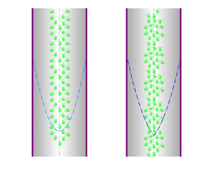
Motile micro-organisms are ubiquitous in various environments and exhibit fascinating phenomena. A classical phenomenon named ‘gyrotactic focusing’ was illustrated in a series of experiments by Kessler (Reference Kessler1984, Reference Kessler1985a,Reference Kesslerb, Reference Kessler1986) using the suspension of Chlamydomonas augustae (mistakenly classified as Chlamydomonas nivalis Bees Reference Bees2020, § 2.1). Gyrotactic focusing describes the centreline-accumulating behaviour of gyrotactic micro-organisms (a micro-organism whose mass centre is located at the far end of the buoyancy centre, e.g. C. augustae) in downwelling pipe flows (Denissenko & Lukaschuk Reference Denissenko and Lukaschuk2007; Bees & Croze Reference Bees and Croze2010; Bearon, Bees & Croze Reference Bearon, Bees and Croze2012; Croze, Bearon & Bees Reference Croze, Bearon and Bees2017; Jiang & Chen Reference Jiang and Chen2020) and channel flows (Croze et al. Reference Croze, Sardina, Ahmed, Bees and Brandt2013). On the contrary, gyrotactic micro-organisms scatter towards the wall in upwelling flows (Kessler Reference Kessler1985a,Reference Kesslerb; Croze et al. Reference Croze, Sardina, Ahmed, Bees and Brandt2013; Fung & Hwang Reference Fung and Hwang2020; Jiang & Chen Reference Jiang and Chen2020). In addition, because micro-organisms are typically heavier than water (Pedley & Kessler Reference Pedley and Kessler1992), the focused micro-organisms in the central region exert an excessive negative buoyant force, thereby accelerating the local flow. This beam is subjected further to instability: when the background flow is weak and the average background cell concentration is high, axisymmetric blips with increased cell concentration and radius compared with the beam were observed (Kessler Reference Kessler1985a, Reference Kessler1986; Denissenko & Lukaschuk Reference Denissenko and Lukaschuk2007).
Predicting the macrotransport process of micro-organisms in an external flow with a precise continuum model is crucial to relevant research and applications, such as understanding aforementioned instabilities (Hwang & Pedley Reference Hwang and Pedley2014a,Reference Hwang and Pedleyb; Saintillan Reference Saintillan2014; Maretvadakethope, Keaveny & Hwang Reference Maretvadakethope, Keaveny and Hwang2019; Bees Reference Bees2020; Fung, Bearon & Hwang Reference Fung, Bearon and Hwang2020; Fung & Hwang Reference Fung and Hwang2020) and optimising the efficiency of artificial cultivation (Chisti Reference Chisti2007). For gyrotactic micro-organisms, Kessler (Reference Kessler1985a,Reference Kesslerb, Reference Kessler1986) introduced a primitive model. He proposed that the swimming directions of micro-organisms are deterministic and shear dependent, and micro-organisms are subject to isotropic diffusion. Kessler (Reference Kessler1985a, Reference Kessler1986) subsequently derived an exponential profile of the steady radial cell concentration distribution in a downwelling pipe flow and analysed the instability. Pedley & Kessler (Reference Pedley and Kessler1990) later proposed a pioneering continuum model, which is denoted as the PK model in the remainder of this paper and also referred to as the FP model by some researchers. Compared with the model of Kessler (Reference Kessler1986), the PK model incorporates biological random reorientation of micro-organisms and gives a more reasonable approximation for anisotropic diffusion in the position space. The PK model first finds the shear-dependent probability density distribution (p.d.f.) of the orientation by solving a Fokker–Planck equation in the orientation space and then uses a semi-empirical direction correlation time to calculate the diffusivity tensor.
Following the same routine to calculate the p.d.f. in the orientation space (and thus average swimming direction) with a specified shear rate, the generalised Taylor dispersion (GTD) theory (Frankel & Brenner Reference Frankel and Brenner1989; Brenner & Edwards Reference Brenner and Edwards1993) was introduced by Hill & Bees (Reference Hill and Bees2002) and Manela & Frankel (Reference Manela and Frankel2003) to derive a more sophisticated but, at the same time, more sensible diffusivity tensor. It should be noted that both the PK model and the GTD model assume that micro-organisms relax in the orientation space with much smaller time and length scales relative to the corresponding scales of micro-organisms swimming in the position space, that is, quasi-steadiness in the orientation space. Bearon, Hazel & Thorn (Reference Bearon, Hazel and Thorn2011) further extended the GTD model to flow fields with inhomogeneous shear, and a quasi-homogeneous assumption is further employed: the shear is slow varying, with time and length scales larger than those of relaxation in the orientation space.
Extensive efforts have been made to test the performance of the PK model and the GTD model. Croze et al. (Reference Croze, Sardina, Ahmed, Bees and Brandt2013) investigated the dispersion of gyrotactic micro-algae in the laminar channel flow with the PK model and the GTD model. Brownian dynamics simulation, in which an individual cell performs a random walk according to the stochastic differential equations (the equivalent of the Smoluchowski equation, i.e. the equation accurately describing the cell's rotation in the orientation space, movement in the position space and the effect of white noise), is employed as a benchmark; the dispersion in the turbulent regime was also simulated using Brownian dynamics simulation. They found that the three models agree well in weak flows, while the GTD model outperforms the PK model in strong flows. The difference originates from the GTD model providing a more rigorous diffusivity tensor than the PK model (Bearon et al. Reference Bearon, Bees and Croze2012; Fung et al. Reference Fung, Bearon and Hwang2020): as the flow becomes stronger, the diffusivity tensor of the PK model approaches a constant scalar matrix asymptotically (in Cartesian coordinates), whereas the diffusivity tensor of the GTD model approaches a zero matrix. Many studies have indicated the superiority of the GTD model over the PK model, not only because of its better accuracy in investigating the dynamics of gyrotactic micro-organisms (Bearon et al. Reference Bearon, Bees and Croze2012; Croze et al. Reference Croze, Sardina, Ahmed, Bees and Brandt2013; Fung et al. Reference Fung, Bearon and Hwang2020; Fung, Bearon & Hwang Reference Fung, Bearon and Hwang2022), but also due to its versatility in studying other kinds of micro-organisms, such as run–tumble chemotactic bacteria (Bearon Reference Bearon2003). Fung et al. (Reference Fung, Bearon and Hwang2020) recently analysed the bifurcation and stability of the suspension of C. augustae in downwelling pipe flows, employing both the GTD model and the PK model for comparison. With the GTD model, a trend consistent with the experimental observation of Kessler (Reference Kessler1986) was found in the variation of stability as a function of the average cell concentration and flow rate; in contrast, the PK model predicted inconsistently.
Despite the foregoing merits, the GTD model has its inherent restriction. This restriction stems from simplifying the fundamental Smoluchowski equation to an advection–diffusion equation in position space. It is important to note that the GTD theory by Frankel & Brenner (Reference Frankel and Brenner1989) was not initially devised to facilitate a position–orientation separation to approximate the Smoluchowski equation. Instead, one should identify all bounded coordinates as the local space and all unbounded coordinates as the global space, and the obtained drift velocity and dispersivity only characterise the dispersion in the global space (Brenner & Edwards Reference Brenner and Edwards1993; Jiang & Chen Reference Jiang and Chen2019, Reference Jiang and Chen2020). Rigorously, the GTD model extended by Hill & Bees (Reference Hill and Bees2002) as well as Manela & Frankel (Reference Manela and Frankel2003) should be only applied to unbounded steady flows with homogeneous shear, and the obtained dispersion coefficients are valid only for long times. When the GTD model facilitating a position–orientation separation is applied to other situations, quasi-steadiness of the orientation dynamics of the micro-organisms, quasi-homogeneity of the flow shear and negligible boundary effect in the position–orientation space must be assumed to obtain an advection–diffusion equation in the position space. For example, Bearon et al. (Reference Bearon, Hazel and Thorn2011) showed the discrepancies between the results of the GTD model and the Smoluchowski-equation-based simulation when the assumptions are not met. In another example, where the distribution of non-biased slender bacteria was considered in a channel flow, Bearon & Hazel (Reference Bearon and Hazel2015) showed how the GTD model predicted a uniform cell concentration profile across the width and failed to reproduce the experimentally observed shear-induced trapping (Rusconi, Guasto & Stocker Reference Rusconi, Guasto and Stocker2014), whereas the results of the full numerical simulation of the Smoluchowski equation are in qualitative agreement with the experimental observations. Bearon & Hazel (Reference Bearon and Hazel2015) then showed a multi-time-scale analysis of the Smoluchowski equation where an effective drift velocity can be derived to explain the shear-induced trapping phenomenon. This multi-time-scale analysis is further formalised by Vennamneni, Nambiar & Subramanian (Reference Vennamneni, Nambiar and Subramanian2020) into an advection–diffusion model, which can capture shear-induced migration of bacteria in a channel flow (Rusconi et al. Reference Rusconi, Guasto and Stocker2014; Barry et al. Reference Barry, Rusconi, Guasto and Stocker2015).
Although the model of Vennamneni et al. (Reference Vennamneni, Nambiar and Subramanian2020) succeeded in capturing shear-induced trapping of micro-organisms, it only works when the motility is not biased, and therefore cannot be extended to case of cells with an orientation bias, such as gyrotactic micro-organisms. This limitation is overcome by the recent work of Fung et al. (Reference Fung, Bearon and Hwang2022), as they first devised an exact transformation of the Smoluchowski equation into an advection–diffusion equation in the position space, before applying a similar multi-time-scale method. In effect, Fung et al. (Reference Fung, Bearon and Hwang2022) has extended the work of Bearon & Hazel (Reference Bearon and Hazel2015) and Vennamneni et al. (Reference Vennamneni, Nambiar and Subramanian2020) by including the effect of biased motility in the multi-time-scale asymptotics. This new model, however, still cannot elude the defects inevitably involved in the position–orientation separation.
As noted previously, the Smoluchowski equation can be referred to as a benchmark for other up-scaled models. Solving the full continuum Smoluchowski equation has therefore also attracted some researchers (Chen & Jiang Reference Chen and Jiang1999; Saintillan & Shelley Reference Saintillan and Shelley2008a,Reference Saintillan and Shelleyb; Ezhilan & Saintillan Reference Ezhilan and Saintillan2015; Jiang & Chen Reference Jiang and Chen2021). However, it is not always possible to resolve the full Smoluchowski equation in a three-dimensional flow field due to numerical difficulty. Only in some simplified circumstances, such as in unidirectional flows, can the dimension of the Smoluchowski equation be reduced. Recently, Jiang & Chen (Reference Jiang and Chen2019) devised the basis functions and solved the Smoluchowski equation in the cross-section of a two-dimensional channel with a Galerkin method. The cross-sectional average drift and diffusivity were accurately derived by directly applying the standard GTD theory (Frankel & Brenner Reference Frankel and Brenner1989; Brenner & Edwards Reference Brenner and Edwards1993) without a position–orientation separation invoking assumptions of quasi-steadiness, quasi-homogeneity and negligible boundary effect. Jiang & Chen (Reference Jiang and Chen2020) further investigated the dispersion of gyrotactic micro-organisms in pipe flows: a detailed comparison with the PK model and the GTD model was presented, explicitly demonstrating the inaccuracy of the PK model and the GTD model when the micro-organisms are highly motile or when the background flow is strong. Alternatively, as a compromised substitute of the Smoluchowski equation, Brownian dynamics simulations are mostly employed for computational convenience (Thorn & Bearon Reference Thorn and Bearon2010; Bearon et al. Reference Bearon, Hazel and Thorn2011; Croze et al. Reference Croze, Sardina, Ahmed, Bees and Brandt2013; Peng & Brady Reference Peng and Brady2020). Although straightforward, if Brownian dynamics simulations are used, one has the problem to include the forces and stresses on the flow induced by the micro-organisms, and these effects are non-negligible in semi-dilute and dense suspensions.
The objective of the present study is to address the buoyancy–flow coupling effect with the transport of micro-organisms directly described by the Smoluchowski equation, hence extending the results in Jiang & Chen (Reference Jiang and Chen2020). In the dilute regime, buoyancy–flow coupling is the dominant effect that negatively buoyant micro-organisms exert on the flow (Pedley & Kessler Reference Pedley and Kessler1990), and is therefore crucial to the transport and stability of the suspension (Bees Reference Bees2020). For the fundamental case within a vertical pipe, there are only a handful of works considering the buoyancy–flow coupling effect. Bees & Croze (Reference Bees and Croze2010) formulated a dispersion scheme resembling the classical Taylor–Aris dispersion theory (Taylor Reference Taylor1953; Aris Reference Aris1956), using the asymptotic results from the PK model. Croze et al. (Reference Croze, Bearon and Bees2017) presented an experimental study and directly compared the measured cross-sectional average drift velocity with predictions from the PK model and the GTD model. The bifurcation and stability in such a configuration were analysed by Fung et al. (Reference Fung, Bearon and Hwang2020) and Fung & Hwang (Reference Fung and Hwang2020) for downwelling and upwelling flows using the PK model and the GTD model. Fung (Reference Fung2021, § 5.1) further performed a bifurcation analysis using an analytical solution of the simplified Smoluchowski equation in a vertical pipe considering the buoyancy–flow coupling effect. Although this solution is still coupled to the Navier–Stokes (N–S) equation (because it is related to the flow profile) and only applies to the steady state of spherical micro-organisms, it offers a more accurate basic state compared with those calculated by the PK model and the GTD model.
In this work, we consider a suspension flowing either downwards or upwards on average. The velocity and cell concentration profiles in the radial direction are assumed to be axially invariant and axisymmetric, as in Bees & Croze (Reference Bees and Croze2010) and Croze et al. (Reference Croze, Bearon and Bees2017). The stability analysis of the solution, such as Fung et al. (Reference Fung, Bearon and Hwang2020) and Fung & Hwang (Reference Fung and Hwang2020), is beyond the scope of this work. Due to the buoyancy–flow coupling effect, the flow velocity profile will deviate from a simple Poiseuille flow and must be solved simultaneously with the Smoluchowski equation. Compared with cases only considering the unidirectional effect of the flow on the cells (Jiang & Chen Reference Jiang and Chen2020), the bidirectional buoyancy–flow interaction couples the velocity and the cell transport, which is the major contribution of this work. In addition, the effect of buoyancy–flow coupling on the dispersion coefficients, namely the drift velocity and the dispersivity, will be discussed. At last, we shall present comparisons between the results of the Smoluchowski equation, the PK model and the GTD model, thus assessing their performances in the presence of the buoyancy–flow coupling effect. This assessment is difficult to realise in the Brownian dynamics simulations.
2. Formulation
2.1. Governing equations
As shown in figure 1, a cylindrical coordinate  $(r^{\ast }, \psi, z^{\ast })$ identified by unit vectors $\boldsymbol {e}_r$, $\boldsymbol {e}_{\psi }$ and $\boldsymbol {e}_z$ characterises the dynamics in the position space and two angles $\theta$ and $\phi$ with the corresponding unit vectors $\boldsymbol {e}_{\theta }$ and $\boldsymbol {e}_{\phi }$ characterise the orientation of a micro-organism. Under the Boussinesq approximation, the N–S equation of the steady, unidirectional, axially invariant and axisymmetric flow velocity $\boldsymbol {u}^{\ast } = U^{\ast }(r^{\ast }) \boldsymbol {e}_z$ is
 \begin{equation} 0 ={-}\frac{1}{\rho^{{\ast}}} \frac{\mathrm{d} p^{{\ast}}}{\mathrm{d} z^{{\ast}}} + \nu^{{\ast}} \frac{1}{r^{{\ast}}} \frac{\mathrm{d}}{\mathrm{d} r^{{\ast}}} \left(r^{{\ast}} \frac{\mathrm{d} U^{{\ast}}}{\mathrm{d} r^{{\ast}}} \right) + n^{{\ast}} v^{{\ast}} \frac{\Delta \rho^{{\ast}}}{\rho^{{\ast}}} g^{{\ast}}.\end{equation}
On the right-hand-side of (2.1), the first term is the imposed pressure gradient ( $\rho ^{\ast }$ is the density of water, and $\mathrm {d} p^{\ast }/\mathrm {d} z^{\ast }$ is the constant pressure gradient along the axial direction $\boldsymbol {e}_z$), the second term is the viscous stress ( $\nu ^{\ast }$ is the kinematic viscosity of water) and the third term is the negative buoyancy of the cells ( $n^{\ast }$ is the cell number density in the position space $(r^{\ast }, \psi, z^{\ast })$, $v^{\ast}$ is the volume of a cell, $\Delta \rho ^{\ast }$ is the density difference between the cell and water and $g^{\ast }$ is the gravitational acceleration).

Figure 1. Sketch of the problem. (a) In an exemplary downwelling flow, the cells accumulate in the central region and thus accelerate the local flow via their negative buoyancy. (b) The top view of the pipe. Unit vectors  $\boldsymbol {e}_r$, $\boldsymbol {e}_{\psi }$ and $\boldsymbol {e}_z$ identify the cylindrical coordinate in the position space. (c) The spherical coordinate characterising the orientation of the micro-organism is featured with a polar angle $\theta$ between $\boldsymbol {p}$ and $\boldsymbol {e}_{\psi }$ and an azimuthal angle $\phi$ between $-\boldsymbol {e}_z$ and the projection of $\boldsymbol {p}$ on the $r$–
$r$– $z$ plane.
In the N–S equation (2.1), the only effect of the micro-organisms on the flow is buoyancy. Here, we further consider the effect of active hydrodynamic stresslet (Saintillan Reference Saintillan2018)
 \begin{equation} \boldsymbol{\varSigma}_p^{{\ast}} = n^{{\ast}} T^{{\ast}} \left(\int \boldsymbol{pp} \frac{f^{{\ast}}}{n^{{\ast}}} \, \mathrm{d}^2 \boldsymbol{p}- \frac{1}{3} {\boldsymbol{\mathsf{I}}}\right), \end{equation}
where  $T^{\ast } = 10^{-10}\ \mathrm {g} \ \mathrm {cm}^2 \ \mathrm {s}^{-2}$ for C. augustae (Pedley Reference Pedley2010; Fung et al. Reference Fung, Bearon and Hwang2020), $\boldsymbol{p}$ is the vector for the orientation of the micro-organism, and $\boldsymbol{\mathsf{I}}$ is the identity tensor. The $z$-component of $(1/\rho ^{\ast })\boldsymbol {\nabla }^{\ast }\boldsymbol {\cdot }\boldsymbol {\varSigma }_p^{\ast }$ is now added to the right-hand side of (2.1). A scaling analysis for the relative strength of the stresslet and buoyancy can be readily achieved by examining $T^{\ast }/(\nu ^{\ast } \Delta \rho ^{\ast } g^{\ast }R^{\ast })$. Substituting the parameters used in this work (shown later in table 1), we obtain a relative strength of $0.01$. Therefore, the stresslet can be safely neglected.
Table 1. Values and ranges of relevant parameters of C. augustae, most of which are taken from Pedley & Kessler (Reference Pedley and Kessler1990) and Hwang & Pedley (Reference Hwang and Pedley2014a,Reference Hwang and Pedleyb).

Assuming that the total number of cells is conserved, the governing equation of the steady-state cell number density  $f^{\ast }$ in the full position–orientation space $(r^{\ast }, \psi, z^{\ast }, \theta, \phi )$, namely the Smoluchowski equation, is
 \begin{equation} \boldsymbol{\nabla}^{{\ast}} \boldsymbol{\cdot} [(\boldsymbol{u}^{{\ast}} + V_s^{{\ast}} \boldsymbol{p} + V_d^{{\ast}} \boldsymbol{e}_z) f^{{\ast}} - D_t^{{\ast}} \boldsymbol{\nabla}^{{\ast}} f^{{\ast}}] + \boldsymbol{\nabla}_p \boldsymbol{\cdot} (\boldsymbol{\dot{p}}^{{\ast}} f^{{\ast}} - D_r^{{\ast}} \boldsymbol{\nabla}_p f^{{\ast}}) = 0. \end{equation}
Here,  $\boldsymbol {\nabla }^{\ast }=\boldsymbol {e}_r (\partial /\partial r^{\ast }) + \boldsymbol {e}_{\psi } (1/r^{\ast })(\partial /\partial \psi ) + \boldsymbol {e}_z (\partial /\partial z^{\ast })$ and $\boldsymbol {\nabla }_p=\boldsymbol {e}_{\theta } (\partial /\partial \theta ) + \boldsymbol {e}_{\phi } (1/\sin \theta ) (\partial /\partial \phi )$ denote the gradient operators in the position space and in the orientation space, respectively; $V_s^{\ast }$ is the swimming velocity of the micro-organisms, with the orientation denoted by $\boldsymbol {p}$; $V_d^{\ast }$ is the settling velocity; $D_t^{\ast }$ and $D_r^{\ast }$ are respectively the intrinsic translational and orientational diffusivities (since we do not consider the hydrodynamic interaction between cells (Ishikawa & Pedley Reference Ishikawa and Pedley2007), these two diffusivities are purely due to the physiology of the micro-organisms); $\boldsymbol {\dot {p}}^{\ast }$ is the time derivative of $\boldsymbol {p}$, and is related to the angular velocity of the micro-organism (denoted by $\boldsymbol {\varOmega }^{\ast }$) via
 \begin{align} \boldsymbol{\dot{p}}^{{\ast}} &= \boldsymbol{\varOmega}^{{\ast}} \times \boldsymbol{p},\nonumber\\ &=\left[\frac{1}{2} \boldsymbol{\omega}^{{\ast}} + \alpha_0 \boldsymbol{p} \times ({\boldsymbol{\mathsf{E}}}^{{\ast}} \boldsymbol{\cdot} \boldsymbol{p}) - \frac{1}{2B^{{\ast}}} (\boldsymbol{p} \times \boldsymbol{e}_z) \right] \times \boldsymbol{p},\nonumber\\ &= \frac{1}{2} \boldsymbol{\omega}^{{\ast}} \times \boldsymbol{p} + \alpha_0 \boldsymbol{p} \boldsymbol{\cdot} {\boldsymbol{\mathsf{E}}}^{{\ast}} \boldsymbol{\cdot} ({\boldsymbol{\mathsf{I}}}- \boldsymbol{pp}) + \frac{1}{2B^{{\ast}}}\boldsymbol{p} (\boldsymbol{p} \boldsymbol{\cdot} \boldsymbol{e}_z) - \frac{1}{2B^{{\ast}}}\boldsymbol{e}_z, \end{align}
with
 \begin{equation} \boldsymbol{\omega}^{{\ast}} = \boldsymbol{\nabla}^{{\ast}} \times \boldsymbol{u}^{{\ast}}, \end{equation}
being the vorticity of the flow, and
 \begin{equation} {\boldsymbol{\mathsf{E}}}^{{\ast}} = \tfrac{1}{2} [\boldsymbol{\nabla}^{{\ast}} \boldsymbol{u}^{{\ast}} + (\boldsymbol{\nabla}^{{\ast}} \boldsymbol{u}^{{\ast}})^{{T}}], \end{equation}
being the rate of strain;  $B^{\ast }$ is the gravitactic reorientation time (smaller for a strong gyrotaxis); $\alpha _0=(\mathcal {AR}^2-1)/(\mathcal {AR}^2+1)$ characterises the shape of the cell ( $\mathcal {AR} \geq 1$ is the aspect ratio of the spheroid). It is important to note that, since the micro-organisms considered in this work are spherical, i.e. $\alpha _0=0$, we have neglected the settling velocity component not parallel to $\boldsymbol {e}_z$ in (2.3), which is, however, non-zero for ellipsoids.
Integrating  $f^{\ast }(r^{\ast }, \theta, \phi )$ over the orientation space yields the cell concentration in the position space, which is denoted by $n^{\ast }$
 \begin{equation} n^{{\ast}}(r^{{\ast}}) \triangleq \int_0^{\rm \pi} \int_0^{2{\rm \pi}} f^{{\ast}} \sin \theta \, \mathrm{d} \phi \, \mathrm{d} \theta. \end{equation}
From here on, we will eliminate the dependences of  $f^{\ast }$ and $n^{\ast }$ on the position coordinates $\psi$ and $z^{\ast }$ using the symmetric and axially invariant assumption.
Dimensionless variables are introduced as
 \begin{equation} \left. \begin{array}{c@{}}
\displaystyle t = \dfrac{t^{{\ast}}
V_s^{{\ast}}}{R^{{\ast}}}, \quad r =
\dfrac{r^{{\ast}}}{R^{{\ast}}}, \quad z =
\dfrac{z^{{\ast}}}{R^{{\ast}}}, \quad D_t =
\dfrac{D_t^{{\ast}}}{V_s^{{\ast}} R^{{\ast}}},\\
\displaystyle D_r=\dfrac{D_r^{{\ast}}
R^{{\ast}}}{V_s^{{\ast}}},\quad \boldsymbol{u} =
\dfrac{\boldsymbol{u}^{{\ast}}}{V_s^{{\ast}}}, \quad
f=\dfrac{f^{{\ast}}}{N^{{\ast}}}, \quad n=
\dfrac{n^{{\ast}}}{N^{{\ast}}},\quad p =
\dfrac{p^{{\ast}}}{{\rho^{{\ast}} V_s^{{\ast}}}^2}, \\
\displaystyle \lambda = \dfrac{1}{2B^{{\ast}}
D_r^{{\ast}}}, \quad Re = \dfrac{R^{{\ast}}
V_s^{{\ast}}}{\nu^{{\ast}}}, \quad Ri =
\dfrac{N^{{\ast}}v^{{\ast}} \Delta \rho^{{\ast}}
g^{{\ast}}R^{{\ast}}}{\rho^{{\ast}}{V_s^{{\ast}}}^2}, \quad
Se = \dfrac{V_d^{{\ast}}}{V_s^{{\ast}}}.
\end{array}\right\} \end{equation}
\begin{equation} \left. \begin{array}{c@{}}
\displaystyle t = \dfrac{t^{{\ast}}
V_s^{{\ast}}}{R^{{\ast}}}, \quad r =
\dfrac{r^{{\ast}}}{R^{{\ast}}}, \quad z =
\dfrac{z^{{\ast}}}{R^{{\ast}}}, \quad D_t =
\dfrac{D_t^{{\ast}}}{V_s^{{\ast}} R^{{\ast}}},\\
\displaystyle D_r=\dfrac{D_r^{{\ast}}
R^{{\ast}}}{V_s^{{\ast}}},\quad \boldsymbol{u} =
\dfrac{\boldsymbol{u}^{{\ast}}}{V_s^{{\ast}}}, \quad
f=\dfrac{f^{{\ast}}}{N^{{\ast}}}, \quad n=
\dfrac{n^{{\ast}}}{N^{{\ast}}},\quad p =
\dfrac{p^{{\ast}}}{{\rho^{{\ast}} V_s^{{\ast}}}^2}, \\
\displaystyle \lambda = \dfrac{1}{2B^{{\ast}}
D_r^{{\ast}}}, \quad Re = \dfrac{R^{{\ast}}
V_s^{{\ast}}}{\nu^{{\ast}}}, \quad Ri =
\dfrac{N^{{\ast}}v^{{\ast}} \Delta \rho^{{\ast}}
g^{{\ast}}R^{{\ast}}}{\rho^{{\ast}}{V_s^{{\ast}}}^2}, \quad
Se = \dfrac{V_d^{{\ast}}}{V_s^{{\ast}}}.
\end{array}\right\} \end{equation}
Here,  $D_t$ and $D_r$ are the dimensionless translational and rotational diffusivities, respectively; $\lambda$ is the dimensionless bias parameter; $f$ and $n$ are respectively the cell p.d.f. in the radius–orientation space $(r,\phi,\theta )$ and the dimensionless cell concentration in the radial direction ( $r$) normalised by the mean cell concentration $N^{\ast }$, thus we have the normalisation condition
 \begin{equation} \int_0^1\int_0^{\rm \pi} \int_0^{2{\rm \pi}} 2 rf\sin \theta \, \mathrm{d} \phi \,\mathrm{d} \theta \,\mathrm{d}r = \int_0^1 2 r n \, \mathrm{d}r = 1; \end{equation} $Re$ is the Reynolds number quantifying the viscous effect; $Ri$ is the Richardson number quantifying the mean cell concentration; and $Se$ is the dimensionless settling velocity.
The dimensionless form of (2.1) is
 \begin{equation} -\frac{\mathrm{d} p}{\mathrm{d} z} + \frac{1}{Re} \frac{1}{r} \frac{\mathrm{d}}{\mathrm{d} r} \left(r \frac{\mathrm{d} U}{\mathrm{d} r} \right)+ Ri \, n= 0, \end{equation}
and the dimensionless form of (2.3) becomes
 \begin{equation} \boldsymbol{\nabla} \boldsymbol{\cdot} [(\boldsymbol{u}+\boldsymbol{p} + Se \boldsymbol{e}_z)f - D_t \boldsymbol{\nabla}f] + \boldsymbol{\nabla}_p \boldsymbol{\cdot} (\boldsymbol{\dot{p}}_r f - D_r \boldsymbol{\nabla}_p f)= 0. \end{equation}
Note that
 \begin{equation} \boldsymbol{\dot{p}}_r = \boldsymbol{\dot{p}} - \boldsymbol{\dot{p}}_c,\end{equation}
is the dimensionless time derivative of  $\boldsymbol {p}$ expressed with basis vectors in the orientation space, namely $\boldsymbol {e}_{\theta }$ and $\boldsymbol {e}_{\phi }$, thus a term
 \begin{equation} \boldsymbol{\dot{p}}_c = \frac{\cos\theta}{r} \boldsymbol{e}_z \times \boldsymbol{p}, \end{equation}
representing the Coriolis effect must be subtracted from  $\boldsymbol {\dot {p}}$ defined in the inertial coordinate. Specifically, $\boldsymbol {\dot {p}}_c$ emerges due to the swimming of micro-organism in the $\boldsymbol {e}_{\psi }$-direction and the dependence of spherical coordinate characterising the orientation of the micro-organism on the cylindrical coordinate fixed in the position space. The angular velocity of the rotating spherical coordinate is $\cos \theta /r \boldsymbol {e}_z$. The detailed expression of $\boldsymbol {\dot {p}}_r$ is
 \begin{equation} \boldsymbol{\dot{p}}_r = \dot{\theta} \boldsymbol{e}_{\theta} + \dot{\phi} \sin\theta \boldsymbol{e}_{\phi}, \end{equation}
where
 $$\begin{gather} \dot{\theta} = \cos\phi \cos\theta \left(D_r \lambda + \alpha_0 \frac{\mathrm{d} U}{\mathrm{d} r} \sin\phi \sin\theta \right) - \frac{\cos\theta \sin\phi}{r}, \end{gather}$$
 $$\begin{gather}\dot{\phi} ={-}\frac{1}{2} \frac{\mathrm{d} U}{\mathrm{d} r} + \frac{1}{2} \alpha_0 \frac{\mathrm{d} U}{\mathrm{d} r} \cos 2\phi - D_r \lambda \csc\theta \sin\phi - \frac{\cos\phi \cos\theta \cot\theta}{r}. \end{gather}$$
 The steady-state Smoluchowski equation (2.11) for the cell p.d.f.  $f(r, \theta, \phi )$ is expressed as
 \begin{align} \mathcal{L} f &\triangleq -\sin\theta \sin\phi \frac{1}{r} \frac{\partial (r f)}{\partial r} - D_t \frac{1}{r} \frac{\partial}{\partial r} \left( r \frac{\partial f}{\partial r}\right) +\frac{1}{\sin\theta} \frac{\partial (\dot{\theta} \sin\theta f)}{\partial \theta} + \frac{\partial (\dot{\phi}f)}{\partial \phi}\nonumber\\ &\quad - D_r \left[ \frac{1}{\sin\theta} \frac{\partial}{\partial \theta} \left( \sin\theta \frac{\partial f}{\partial \theta} \right) + \frac{1}{\sin^2\theta} \frac{\partial^2 f}{\partial \phi^2} \right] = 0, \end{align}
where  $\mathcal {L}$ denotes the operator characterising the transport in the radius–orientation space $(r, \theta, \phi )$.
2.2. Solutions for velocity and cell p.d.f.
The total flow rate is calculated by
 \begin{equation} Q = \int_0^1 2 {\rm \pi}rU(r) \, \mathrm{d}r ={\rm \pi} U_m, \end{equation}
where  $U_m$ denotes the mean flow velocity. We shall prescribe the mean flow velocity $U_m$, then there are two variables $U(r)$ and $f(r, \theta, \phi )$ along with (2.10) and (2.17). Theoretically, the coupled equations can be solved with appropriate constraints and boundary conditions.
The boundary conditions for  $U(r)$ are a no-slip condition at the wall and a boundedness condition at the centreline
 $$\begin{gather} U(1) = 0, \end{gather}$$
 $$\begin{gather}U(0) \neq \infty. \end{gather}$$
 For  $f(r, \theta, \phi )$, following Jiang & Chen (Reference Jiang and Chen2020), we use specular reflection boundary conditions to ensure the no-flux requirement of cell concentration at the wall
 $$\begin{gather} f(r, \theta, \phi, t)|_{r=1} = f(r, \theta, -\phi, t)|_{r=1}, \end{gather}$$
 $$\begin{gather}\left. \frac{\partial f(r, \theta, \phi, t)}{\partial r}\right|_{r=1} =\left. -\frac{\partial f(r, \theta, -\phi, t)}{\partial r}\right|_{r=1}. \end{gather}$$
We note that the reflection boundary conditions may not be appropriate for micro-organisms featuring wall adhesion, for example, non-biased bacteria accumulate at walls (Berke et al. Reference Berke, Turner, Berg and Lauga2008; Li & Tang Reference Li and Tang2009). However, we suppose that the reflection boundary conditions are suitable for a vertical pipe configuration, because most of the suspended gyrotactic micro-organisms accumulate in the central region in a downwelling flow and the high shear rate at the wall dominates the reorientation of cells in an upwelling flow. Furthermore, as noted previously, the PK model and the GTD model are unable to incorporate boundary conditions in the position–orientation space, and no-flux boundary conditions in the position space are imposed; therefore, using the reflection boundary conditions does not affect the comparisons between the PK model, the GTD model and the Smoluchowski equation (Bearon et al. Reference Bearon, Hazel and Thorn2011; Croze et al. Reference Croze, Sardina, Ahmed, Bees and Brandt2013; Bearon & Hazel Reference Bearon and Hazel2015; Jiang & Chen Reference Jiang and Chen2020).
The boundedness condition for  $\theta$ is
 \begin{equation} f|_{\theta=0} \neq \infty, \quad f|_{\theta={\rm \pi}} \neq \infty, \end{equation}
and the periodic boundary conditions for  $\phi$ are
 $$\begin{gather} f_{\phi=2 {\rm \pi}} = f|_{\phi=0}, \end{gather}$$
 $$\begin{gather}\frac{\partial f}{\partial \phi}\bigg|_{\phi=2 {\rm \pi}} = \frac{\partial f}{\partial \phi}\bigg|_{\phi=0}. \end{gather}$$
In this work, we shall use a Galerkin method for the Smoluchowski equation and an eigenfunction expansion method for the N–S equation. To resolve the buoyancy–flow coupling, an iterative method is employed (Hwang & Pedley Reference Hwang and Pedley2014b). The details of the numerical method are given in Appendix A.
2.3. Solutions for dispersion coefficients
The drift velocity  $U_d$ and the dispersivity $D_{{T}}$ constitute two key parameters in the drift–dispersion equation for the cross-sectional average cell concentration at the asymptotically long time. However, care must be taken in understanding these two coefficients in the current situation: they only describe the dispersion of a small number of labelled cells in an existing background flow formed by the imposed flow and a large number of unlabelled cells. Specifically, compared with the unlabelled cells, the distortion on the flow induced by the labelled cells is negligible. This assumption decouples the dispersion of labelled cells from the background buoyancy–flow coupling problem and ensures the background flow is always steady (Bees & Croze Reference Bees and Croze2010; Croze et al. Reference Croze, Bearon and Bees2017), which are required for the application of Taylor–Aris theory (Taylor Reference Taylor1953; Aris Reference Aris1956; Guan et al. Reference Guan, Zeng, Jiang, Guo, Wang, Wu, Li and Chen2022; Jiang et al. Reference Jiang, Zeng, Fu and Wu2022) and the GTD theory (Frankel & Brenner Reference Frankel and Brenner1989; Brenner & Edwards Reference Brenner and Edwards1993; Jiang & Chen Reference Jiang and Chen2019, Reference Jiang and Chen2020).
With the solved velocity profile  $U(r)$ and cell p.d.f. profile $f(r, \theta, \phi )$, one can apply the standard GTD theory (Frankel & Brenner Reference Frankel and Brenner1989; Jiang & Chen Reference Jiang and Chen2019, Reference Jiang and Chen2020) to evaluate the cross-sectional average drift velocity $U_d$ and dispersivity $D_{{T}}$. Let $\langle ({\cdot }) \rangle$ denote the integration $2 \int _0^1 \int _0^{{\rm \pi} } \int _0^{2{\rm \pi} } ({\cdot }) r \sin \theta \, \mathrm {d} \phi \,\mathrm {d} \theta \,\mathrm {d} r$, the cross-sectional average drift velocity $U_d$ and dispersivity $D_{{T}}$ are calculated by Jiang & Chen (Reference Jiang and Chen2020, (3.34) and (3.35))
 $$\begin{gather} U_d = \langle V_z(r, \theta, \phi) f(r, \theta, \phi) \rangle, \end{gather}$$
 $$\begin{gather}D_{{T}} = D_t + \langle V_z(r, \theta, \phi) b(r, \theta, \phi) \rangle, \end{gather}$$
where
 \begin{equation} V_z(r, \theta, \phi) = U(r) + p_z(\theta, \phi) + Se = U(r) - \sin\theta \cos\phi + Se, \end{equation}
is the local effective velocity, and  $b(r, \theta, \phi )$ is a scalar field constituting the solution of the equation (Frankel & Brenner Reference Frankel and Brenner1989; Brenner & Edwards Reference Brenner and Edwards1993; Haugerud, Linga & Flekkøy Reference Haugerud, Linga and Flekkøy2022)
 \begin{equation} \mathcal{L} b = f(V_z - U_d).\end{equation}
An additional normalisation condition for  $b(r, \theta, \phi )$ is imposed to ensure its uniqueness
 \begin{equation} \langle b(r, \theta, \phi) \rangle =0,\end{equation}
note that this normalisation condition does not affect the dispersivity. Then  $b(r, \theta, \phi )$ is also solved by a Galerkin method (see Appendix A for details).
3. Results and discussion
Following Jiang & Chen (Reference Jiang and Chen2020), among others (Pedley & Kessler Reference Pedley and Kessler1992; Bees & Hill Reference Bees and Hill1998; Hwang & Pedley Reference Hwang and Pedley2014a,Reference Hwang and Pedleyb; Zeng & Pedley Reference Zeng and Pedley2018), parameters of the gyrotactic species C. augustae are used for calculation to illustrate the buoyancy–flow coupling effect, as listed in table 1.
It is noteworthy that, at high flow rate, the Richardson number  $Ri$ must be below a threshold $Ri_c$ to avoid blow-up of the focused beam, i.e. to ensure the existence of a steady solution. We adopt a formula from Fung et al. (Reference Fung, Bearon and Hwang2020, § 3.3) to estimate this threshold, that is, $Ri_c=16/(\lambda Re)$. This formula is deduced using the analytical solution of the simplified Smoluchowski equation (Fung Reference Fung2021, § 5.1), and can be also obtained from a simplified model resembling the GTD model. Substituting the values of $\lambda$ and $Re$ in our case, we obtain $Ri_c=122.85$. If $Ri$ is larger than $Ri_c$ at a high flow rate, a steady solution may not exist and the numerical method in this work becomes invalid. It is acknowledged that this threshold numerically estimated by the full Smoluchowski equation may slightly differ from the one given by the formula which assumes that all cells are concentrated in a narrow core around the axis; however, since the bifurcation structure is not the focus of this work, we do not try to find out the exact $Ri_c$ and an upper limit of $Ri=100$ is tested to guarantee a steady solution.
3.1. Velocity and cell concentration profiles
We first report the results in downwelling flows, as shown in figure 2 (the profiles of the velocity deviation above the mean) and figure 3 (the cell concentration profiles) for three Richardson numbers ( $Ri=0$, $36.6$ and $73.1$) and three mean flow velocities ( $U_m=1$, $5$ and $10$). The velocity deviation above the mean is defined as
 \begin{equation} \chi(r) = \frac{U(r)}{U_m}-1. \end{equation}
Figure 2. The velocity deviation profiles  $\chi (r)$ in the downwelling flows with $Ri=0$, $36.6$ and $73.1$. The cell transport is calculated using the Smoluchowski equation; (a) $U_m=1$, (b) $U_m=5$, (c) $U_m=10$.

Figure 3. The cell concentration profiles  $n(r)$ in the downwelling flows with $Ri=0$, $36.6$ and $73.1$. The cell transport is calculated using the Smoluchowski equation; (a) $U_m=1$, (b) $U_m=5$, (c) $U_m=10$.
As seen in figure 2, when  $Ri=0$, i.e. the buoyancy–flow coupling effect vanishes and the velocity profile is completely decoupled from the cell concentration profile, the flow is exactly a Poiseuille flow characterised by $\chi (0)=1$ and $\chi (1)=-1$ with $r=0$ and $1$ corresponding to the centreline and wall, respectively. As $Ri$ increases, we see that the flow profile deviates from the Poiseuille flow, as evidenced by an increased velocity at the centreline ( $\chi (0)>1$). In addition, we observe that $\chi (0)$ varies non-monotonically with $U_m$ when $Ri$ is set to positive (see also figure 5c), indicating a competition between the buoyancy–flow coupling effect and the background flow. We shall investigate this non-monotonicity quantitatively later. The cell concentration profiles typical of gyrotactic focusing at the central region in the downwelling flows are depicted in figure 3. The increases of both $U_m$ and $Ri$ have a profound enhancement on the gyrotactic focusing, as reflected by the increased cell concentration at the centreline.
Now we turn to the upwelling flows, the velocity deviation profiles with  $U_m=-10$ are shown in figure 4(a). We find no discernible difference between the profiles obtained with different $Ri$ at this selected $U_m$, which is relatively large, i.e. profiles almost identical to an upwelling Poiseuille flow are predicted. This observation is the key result in the upwelling cases, and is also in deep contrast to the downwelling cases where the buoyancy–flow coupling effect has a significant influence on the velocity deviation profile even when $|U_m|=10$. In the upwelling flows, the gyrotactic cells scatter towards the wall where they were expected to distort the flow via their negative buoyancy. Nonetheless, near the wall, the no-slip condition (2.19) dominates the buoyancy–flow coupling effect, and thus the velocity deviation profiles do not vary as much as they do in the downwelling cases when $Ri$ is increased. Although we see in figure 5(c) that the buoyancy–flow coupling effect still accelerates the peripheral flow (in the $\boldsymbol {e}_x$ direction) and consequently leads to an increased velocity deviation at the centreline ( $\chi (0)>1$), this effect vanishes faster than that in the downwelling flows as $|U_m|$ increases. We present the cell concentration profiles in the upwelling flows with $U_m=-10$ in figure 4(b), and the almost identical cell concentration profiles at different $Ri$ can be understood by the almost identical velocity deviation profiles. Meanwhile, since micro-organisms are mostly located in the near-wall region where the buoyancy–flow coupling effect is insignificant, we do not see a notable difference between the cell concentration at the wall $n(1)$ at different $Ri$ as shown in figure 5(b).

Figure 4. (a) The velocity deviation profiles  $\chi (r)$. (b) The cell concentration profiles $n(r)$ in the upwelling flows. The cell transport is calculated using the Smoluchowski equation. Note that the velocity deviation profiles $\chi (r)$ at all sampled mean flow velocity ( $U_m=-1$, $-5$ and $-10$) are very close, and therefore only profiles with $U_m=-10$ are shown here.

Figure 5. (a) Variations of the cell concentration at the centreline  $n(0)$ as a function of the mean velocity $U_m$ in the downwelling flows. (b) Variations of the cell concentration at the wall $n(1)$ as a function of the mean velocity $U_m$ in the upwelling flows. (c) Variations of the velocity deviation at the centreline $\chi (0)$ as a function of the mean velocity $U_m$. Here, ‘S’, ‘G’ and ‘P’ denote results obtained from the Smoluchowski equation, the GTD model and the PK model, respectively.
As noted previously, there exists a competition between the buoyancy–flow coupling effect and the background flow, as evidenced by the non-monotonic variation of  $\chi (0)$ with increasing $U_m$ (see e.g. figures 3 and 5a): $\chi (0)$ first experiences an increase and then a decrease to unity as $U_m$ increases when $Ri>0$. An intuitive impression on the strength of the buoyancy–flow coupling effect in the $U_m$– $Ri$ plane is given in figure 6, where the contours of the velocity deviation at the centreline $\chi (0)$ and the cell concentration at the centreline $n(0)$ are plotted. We observe that, while $\chi (0)$ increases monotonically with $Ri$ regardless of the value of $U_m$, $\chi (0)$ is maximally enhanced at a moderate $U_m$ (approximately equals $2$). In contrast, $n(0)$ increases monotonically with both $U_m$ and $Ri$.
$Ri$.

Figure 6. Contours of (a) the velocity deviation at the centreline  $\chi (0)$ and (b) the cell concentration at the centreline $n(0)$ in the $U_m$– $Ri$ plane.
3.2. Drift velocity and dispersivity
Figure 7 illustrates the variations of the drift velocity  $U_d$ and the dispersivity $D_{{T}}$ as functions of the mean flow speed $U_m$ for three Richardson numbers ( $Ri=0$, $36.6$ and $73.1$). In the downwelling flows, $U_d$ increases monotonically with $U_m$ and $Ri$. This trend can be well understood by the accelerated flow velocity and concentrated cell concentration in the central region, both of which contribute to a larger $U_d$. For $D_{{T}}$, we observe a boost with increasing $Ri$, which can be probably explained by the enhanced shear in the central region benefiting dispersion; however, since $D_{{T}}$ is a quantity related to the complex scalar field $b(r, \theta, \phi )$, an intuitive understanding of its variation with the flow strength and the cell concentration profile is potentially difficult. For example, as shown in figure 7(a), in the downwelling flows, $D_{{T}}$ exhibits a non-monotonic variation with $U_m$: $D_{{T}}$ first increases and then decreases as $U_m$ increases, which is also reported in non-coupling cases (Croze et al. Reference Croze, Sardina, Ahmed, Bees and Brandt2013; Jiang & Chen Reference Jiang and Chen2020) and coupling cases (Croze et al. Reference Croze, Bearon and Bees2017). This non-monotonic variation is due to the effect of the enhanced gyrotactic focusing on the dispersion. We shall consider two extreme cases to understand this variation: first, there is no flow, and thus dispersivity $D_{{T}}$ is solely contributed by swimming, which is very small due to biased swimming induced by gyrotaxis; second, there is an extremely strong flow, and thus nearly all the cells are located in the centre, meaning that differential advection again contributes nothing to dispersivity; between these two extremes, the dispersivity is increased by both the swimming-induced dispersion and differential-advection-induced dispersion.

Figure 7. Variations of drift velocity  $U_d$ and dispersivity $D_{{T}}$ as functions of the mean velocity $U_m$ (a,b) in the downwelling flows and (c,d) in the upwelling flows. Here, ‘S’, ‘G’ and ‘P’ denote results obtained from the Smoluchowski equation, the GTD model and the PK model, respectively.
In the upwelling flows,  $U_d$ is negative because both the advective velocity of the background flow and the average swimming velocity of the gyrotactic micro-organisms are directed upwards. In contrast to the downwelling cases, $U_d$ finally saturates in the upwelling flows. A sensible explanation for this phenomenon is that, in the limit of extremely strong upwelling flow, all micro-organisms scatter towards the wall, thus $U_d$ is independent of $U_m$ and is solely determined by the near-wall orientation distribution of the micro-organisms (which determines the swimming-induced drift). The non-monotonic variation of $D_{{T}}$ with $U_m$ in the upwelling flows is analogous to that observed in the downwelling flows, and is also due to an initial increment and a following reduction of the differential-advection-induced dispersion as the flow becomes strong. Although the buoyancy–flow coupling effect is relatively weak in the upwelling flows because of the dominance of the no-slip wall, we are still able to observe slight differences of $U_d$ and $D_{{T}}$ between cases with different $Ri$ at a moderate range of $U_m$ (around $2$). It is seen that $U_d$ is increased with a larger $Ri$, this is due to the fact that the micro-organisms now accelerate the flow near the wall in the $\boldsymbol {e}_x$ direction, while the background flow is in the $-\boldsymbol {e}_x$ direction; this counteracting effect finally leads to the increase of $U_d$ with $Ri$. The decrease of $D_{{T}}$ with $Ri$ can be probably also understood by the modification on the flow profile: the shear in the near-wall region where the micro-organisms accumulate is decreased, and thus the contribution of differential advection to the dispersion is weakened.
3.3. Comparisons with PK model and GTD model
For dispersion of gyrotactic micro-organisms in a pipe, we can employ a simplified method for the calculation using the PK model and the GTD model, see e.g. Bearon et al. (Reference Bearon, Bees and Croze2012, Appendix E). Now using the parameters of C. augustae and the calculation method presented in Appendix B, we shall compare the results obtained from the Smoluchowski equation with those from the PK model and the GTD model (the comparisons are already included in figure 5 and figure 7). It is also noteworthy that Croze et al. (Reference Croze, Bearon and Bees2017) used a different species called Dunaliella salina in their experiment. We note that  $\lambda =0.21$ for D. salina, which means that their gyrotactic focusing will be weak, and thus the effect of buoyancy–flow coupling will be less significant. In Appendix C, we present the comparisons between the results of D. salina calculated using the PK model, the GTD model, the Smoluchowski equation and the results measured in the experiments.
We first discuss the comparisons in the downwelling flows. As shown in figure 5(a), when  $Ri=0$, the Smoluchowski equation and the GTD model predict almost the same $n(0)$ profiles, typical of gyrotactic focusing, while $n(0)$ predicted by the PK model is very close to unity. As $Ri$ increases, we see that the flow deviates from a Poiseuille flow for all models, as evidenced by an increased velocity at the centreline $\chi (0)>1$ (figure 5c). However, the buoyancy–flow coupling effect is less profound predicted by the PK model, while the GTD model slightly overestimates the effect at a moderate $U_m$ and underestimates it at a large $U_m$. The unsatisfactory performance of the PK model in high-shear flows has long been recognised (Croze et al. Reference Croze, Sardina, Ahmed, Bees and Brandt2013, Reference Croze, Bearon and Bees2017; Bees Reference Bees2020; Fung et al. Reference Fung, Bearon and Hwang2020; Jiang & Chen Reference Jiang and Chen2020). This weakness is because the diffusion tensor calculated by the PK model cannot reflect the shear-induced dispersion in the position space (Croze et al. Reference Croze, Sardina, Ahmed, Bees and Brandt2013). In a Poiseuille flow, if the flow rate continues increasing, the cell concentration profile predicted by the PK model will tend to be uniform, e.g. Bearon et al. (Reference Bearon, Bees and Croze2012, figure 2) and Croze et al. (Reference Croze, Bearon and Bees2017, figure 1a), as a result of the mean swimming velocity approaching to zero and the diffusivity tensor approaching to a constant scalar matrix (in Cartesian coordinate). In other words, gyrotactic micro-organisms will behave in a similar manner to passive tracers if one applies the PK model in a high-shear flow. For the buoyancy–flow coupling effect, although the velocity deviation at the centreline $\chi (0)$ does reflect the buoyancy–flow coupling effect to some extent, we do not see a noteworthy variation of $n(0)$ as $Ri$ increases with the PK model.
The velocity deviation at the centreline  $\chi (0)$ predicted by the Smoluchowski equation and the GTD model are close (figure 5c). Nonetheless, when it turns to the cell concentration at the centreline $n(0)$, an apparent difference is seen when $Ri > 0$, as is seen in figure 5(a). The GTD model underestimates the gyrotactic focusing in the presence of the buoyancy–flow coupling effect. This result is due to these models sharing the same governing equation for the flow but fundamentally different governing equations for the cell transport (Bees Reference Bees2020). In the analytical solution of the Smoluchowski equation (Fung Reference Fung2021, § 5.1) and in models assuming a position–orientation separation, the radial cell concentration has an exponential scaling with the flow profile (see e.g. Fung Reference Fung2021, (5.1)) or the ratio between the radial components of the local drift velocity and the diffusivity tensor (see e.g. (B6)), which also depends on the flow profile. Thus, any perturbation on the flow profile will result in a remarkable change in the cell concentration, causing the cell concentration to be more sensitive to the models.
Now we turn to cases where the flow is upwards, the comparisons of the velocity deviation at the centreline  $\chi (0)$ and the cell concentration at the wall $n(1)$ with varying $U_m$ are shown in figures 5(c) and 5(b). We find that all models predict almost identical $\chi (0)$. Furthermore, as the flow becomes strong, $\chi (0)$ values obtained with all models approach unity. This coincidence is again in deep contrast with the downwelling cases where the cell transport model has a significant influence on $\chi (0)$, and can be also attributed to the no-slip boundary condition imposed at the wall. For $n(1)$, we see relatively good agreement between the predictions of the Smoluchowski equation and the GTD model at weak and moderate flow strengths, deviation is, however, observed in strong flow. In contrast, the PK model yields a much more uniform concentration profile and a decreasing trend of $n(1)$ as the flow becomes strong when $U_m$ is smaller than $-2$.
$-2$.
Figure 7(a) compares the variations of the drift velocity  $U_d$ as functions of the mean flow speed $U_m$ in the downwelling flows between different models. We see that $U_d$ predicted by the GTD model and the Smoluchowski equation are nearly twice as large as the one predicted by the PK model with a large $U_m$. This is because both the GTD model and the Smoluchowski equation can effectively capture the gyrotactic focusing phenomenon in a strong flow. Specifically, cells accumulate at the centreline where the local advective speed is twice the mean flow velocity in non-coupling cases. In contrast, $U_d$ predicted by the PK model gradually approaches $U_m$, as a consequence of the nearly uniform radial cell concentration profile resembling that of solute tracers. For the effect of buoyancy–flow coupling, we see that the GTD model and the Smoluchowski equation still give almost identical $U_d$ (figure 7a). Although we have seen that the cell concentration at the centreline $n(0)$ of the Smoluchowski equation is significantly larger than that of the GTD model (figure 5a), this concentration enhancement in the central region does not lead to a discernible increase of $U_d$, since the area of the narrow central core scales with $r^2$. In addition, the curves of the PK model at all sampled $Ri$ nearly overlap except for a very small $U_m$.
The variation of dispersivity  $D_{{T}}$ as a function of the mean flow speed $U_m$ in the downwelling flows between different models is presented in figure 7(b). Different from the results of the Smoluchowski equation, the GTD model predicts a saturated instead of a decreasing $D_{{T}}$. In contrast, although the PK model captures the variation of $D_{{T}}$ with increasing $Ri$, it fails to reflect neither the decrease nor the saturation of $D_{{T}}$ when the flow becomes strong. In summary, for the cases in the downwelling flows, the GTD model outperforms the PK model, but still overestimates $D_{{T}}$.
The dispersion predictions in the upwelling flows by different models are plotted in figures 7(c) and 7(d). First, although  $U_d$ of the GTD model finally becomes nearly a constant with an initial drop as $|U_m|$ increases, an extra turning point is observed compared with the curve predicted by the Smoluchowski equation. In comparison, the curves of the PK model still behave very differently from the other two models: a tracer-like dispersion behaviour is predicted again as $|U_m|$ increases. For the dispersivity $D_{{T}}$, although the GTD model also predicts a non-monotonic trend as the flow becomes strong, the agreement with the results of the Smoluchowski equation remains qualitative.
4. Concluding remarks
In this paper, by solving the N–S equation and the Smoluchowski equation simultaneously, we investigate the effect of buoyancy–flow coupling on the velocity profile, cell concentration profile and Taylor dispersion of a suspension of gyrotactic micro-organisms in a vertical pipe. The buoyancy–flow coupling effect is more significant when the average flow is directed downwards, as a consequence of gyrotactic focusing of negatively buoyant micro-organisms accelerating the flow in the central region. In contrast, the buoyancy–flow coupling effect has a minor influence in the upwelling flows because the negative buoyancy of the wall-accumulated micro-organisms is inferior to the effect of the no-slip condition imposed at the wall. In the downwelling flows, the buoyancy–flow coupling effect leads to enhanced flow velocity and gyrotactic focusing in the central region, as well as enhanced drift velocity and dispersivity. The strength of the buoyancy–flow coupling effect can be quantified by the Richardson number  $Ri$; however, its modification to the flow, which we use the velocity deviation at the centreline $\chi (0)$ to quantify, is largest at a moderate mean flow velocity $U_m$. This phenomenon is understood by considering that a small $U_m$ does not arouse obvious gyrotactic focusing and thus the cell concentration is too uniform to result in acceleration of the flow in the central region, while a large $U_m$ due to the imposed pressure gradient overwhelms the buoyancy–flow coupling effect.
Another contribution of this paper is giving a benchmark test for the PK model and the GTD model in the presence of the buoyancy–flow coupling effect. It has been shown in previous studies that the PK model performs unsatisfactorily in strong shear flows (Croze et al. Reference Croze, Sardina, Ahmed, Bees and Brandt2013, Reference Croze, Bearon and Bees2017; Jiang & Chen Reference Jiang and Chen2020). Here, we further confirm its defect in the presence of the buoyancy–flow coupling effect. In comparison, although the GTD model captures some trends in the variations, its predictions of the dispersivity still deviate a lot from the exact results of the Smoluchowski equation.
One may inevitably question the extent to which the Smoluchowski equation can explain the pioneering experimental measurements in Croze et al. (Reference Croze, Bearon and Bees2017). We show the comparisons in Appendix C; however, no obvious improvement on the GTD model is seen, since  $\lambda =0.21$ for D. salina and thus assumptions of the GTD model basically hold. Although somewhat disappointed, we still advocate using the Smoluchowski equation in relevant problems, at least as a benchmark test, because we have shown the inaccuracy of the GTD model when the assumptions associated with orientation–position separation are not met. The fact that the experimental results do not agree satisfactorily with the GTD model and the Smoluchowski equation is open to many possible explanations, such as heterogeneity of micro-organisms (Bees, Hill & Pedley Reference Bees, Hill and Pedley1998), cell–cell interactions in the central core (Fung et al. Reference Fung, Bearon and Hwang2020) and the microscopic kinematic model of the cell (Omori et al. Reference Omori, Kikuchi, Schmitz, Pavlovic, Chuang and Ishikawa2022; Walker et al. Reference Walker, Ishimoto, Moreau, Gaffney and Dalwadi2022; Zeng, Jiang & Pedley Reference Zeng, Jiang and Pedley2022), which deserve in-depth research.
Another important issue not covered by the current study is the possible bifurcation and stability of the steady-state solutions. Since we have limited the Richardson number  $Ri$ to less than $100$, we can safely evade the regimes with bifurcation and instability. It is of great interest to extend the current work to linear hydrodynamic stability analysis of the solutions; however, great difficulty arises in converting the linearised equation to an eigenvalue problem due to the non-parallel perturbed flow field and complex axial transport of cells. Fung (Reference Fung2021, § 5.1) has given a preliminary analysis and this problem should be explored in future work.
Acknowledgements
We are especially grateful for the constructive comments from three anonymous referees. We also thank Professor L. Zeng and M.Y. Guan for helpful inputs.
Funding
This work is supported by the National Natural Science Foundation of China (Grant Nos. 52079001 and 52109093). W.J. acknowledges the support of China Postdoctoral Science Foundation (Grant Nos. 2021M701906 and 2022T150362).
Declaration of interests
The authors report no conflict of interest.
Appendix A. Numerical method
In this appendix, we show the numerical method for solving (2.10) and (2.17).
For the N–S (2.10), we use the eigenfunction expansion method. The basis functions for  $U(r)$ are adopted as the eigenfunctions of operator
 \begin{equation} \varDelta_r = \frac{1}{r} \frac{\partial }{\partial r} \left( r \frac{\partial }{\partial r}\right), \end{equation}
and are found to be
 \begin{equation} R_i^{{D}}(r) = \sqrt{2} \frac{{J}_0 (\gamma_i r)}{{J}_1 (\gamma_i)}, \quad i=1,2,\ldots. \end{equation}
Here, the superscript ‘ ${D}$’ denotes the Dirichlet boundary condition (2.19) at $r=1$; ${J}_0$ and ${J}_1$ are the Bessel functions of order $0$ and $1$, respectively; $\gamma _i$ is the $i$th zero of
 \begin{equation} {J}_0 (\gamma_i) = 0, \quad i=1,2,\ldots, \end{equation}
and the corresponding eigenvalue is  $-\gamma _i^2$ ( $\varDelta _r R_i^{{D}}=-\gamma _i^2 R_i^{{D}}$).
For the Smoluchowski equation (2.17), a Galerkin method is employed. The basis functions for  $f(r, \theta, \phi )$ are adopted as the eigenfunctions of operator
 \begin{equation} \varDelta_q = \frac{1}{r} \frac{\partial }{\partial r} \left( r \frac{\partial }{\partial r}\right) + \frac{1}{\sin\theta} \frac{\partial}{\partial \theta} \left(\sin\theta \frac{\partial}{\partial \theta} \right) + \frac{1}{\sin^2\theta} \frac{\partial^2}{\partial \phi^2}, \end{equation}
and take the form of (Jiang & Chen Reference Jiang and Chen2020, § 3.2.1)
 $$\begin{gather} R^{{N}} (r) \sqrt{\frac{2l+1}{4{\rm \pi}}} {P}_l (\cos\theta), \end{gather}$$
 $$\begin{gather}R^{{N}} (r) \sqrt{2} \sqrt{\frac{2 l+1}{4{\rm \pi}} \frac{(l-m)!}{(l+m)!}} \cos(m\phi) {P}_l^m(\cos\theta), \quad m=1,2, \ldots, l, \end{gather}$$
 $$\begin{gather}R^{{D}} (r) \sqrt{2} \sqrt{\frac{2 l+1}{4{\rm \pi}} \frac{(l-m)!}{(l+m)!}} \sin(m\phi) {P}_l^m(\cos\theta), \quad m=1,2, \ldots, l, \end{gather}$$
where  $l=0,1,2, \ldots$. Here, ${P}_l$ are the Legendre polynomials and ${P}_l^m$ are the associated Legendre polynomials,
 \begin{equation} {P}_l^m(x) = ({-}1)^m (1-x^2)^{m/2} \frac{\mathrm{d}^m}{\mathrm{d} x^m} {P}_l(x); \end{equation}
where  $R^{{N}}(r)$ is the eigenfunctions of the operator $\varDelta _r$ (A1) with Neumann boundary conditions (‘ ${N}$’ denotes Neumann boundary condition), thus we obtain
 \begin{equation} R^{{N}}_i(r) = \sqrt{2} \frac{{J}_0 (\beta_i r)}{{J}_0 (\beta_i)},\quad i=1,2, \ldots, \end{equation}
where  $\beta _i$ is determined by
 \begin{equation} {J}_1(\beta_i) = 0, \quad i=1,2, \ldots. \end{equation}
 We denote the basis of  $f(r, \theta, \phi )$ as $\{e_j(r, \theta, \phi )\}_{j=1}^{N_f}$, where $N_f$ is the truncation degree; $f(r, \theta, \phi )$ is subsequently expanded into
 \begin{equation} f(r, \theta, \phi) \approx \sum_{j=1}^{N_f} a_j e_j(r, \theta, \phi). \end{equation}
Similarly,  $U(r)$ is expanded into
 \begin{equation} U(r) \approx \sum_{j=1}^{N_u} b_j R_j^{{D}}(r). \end{equation}
For the buoyancy–flow coupling problem (2.10) and (2.17) are rewritten abstractly as
 $$\begin{gather} \mathcal{T}(f, U) = 0, \end{gather}$$
 $$\begin{gather}\mathcal{M}(f, U) = 0. \end{gather}$$
The solution procedure is summarised as follows:
(i) Assign an initial guess denoted by $U^0(r)$ to $U(r)$. Here, we use a Poiseuille flow first,
(A15)where\begin{equation} U^0(r) = 2 U_m (1-r^2) \approx \sum_{j=1}^{N_u}b_j^0 R_j^{{D}}(r), \end{equation}(A16)by orthogonality of the eigenfunctions.\begin{equation} b_j^0 = 2 U_m \int_0^1 (1-r^2) r R_j^{{D}} (r) \,\mathrm{d} r, \end{equation}
$U^0(r)$ to $U(r)$. Here, we use a Poiseuille flow first,
(A15)where\begin{equation} U^0(r) = 2 U_m (1-r^2) \approx \sum_{j=1}^{N_u}b_j^0 R_j^{{D}}(r), \end{equation}(A16)by orthogonality of the eigenfunctions.\begin{equation} b_j^0 = 2 U_m \int_0^1 (1-r^2) r R_j^{{D}} (r) \,\mathrm{d} r, \end{equation}(ii) Substitute
$U^0(r)$ into the Smoluchowski equation (A13)
(A17)and obtain\begin{equation} \mathcal{T}(f^0;U^0)=0, \end{equation}$f^0(r, \theta, \phi ) \approx \sum _{j=1}^{N_f} a_j^0 e_j(r, \theta, \phi )$. The coefficients $\{a_j\}_{j=1}^{N_f}$ are solved with a Galerkin method, as detailed in Jiang & Chen (Reference Jiang and Chen2020).(iii) Substitute
$f^0(r, \theta, \phi )$ into the momentum equation (A14)
(A18)and use the eigenfunction expansion method with the constraint (2.18) to solve\begin{equation} \mathcal{M}(U^1;f^0)=0, \end{equation}$U^1(r) \approx \sum _{j=1}^{N_u} b_j^1 R_j^{D}(r)$.(iv) Repeat steps (ii) and (iii) for numerical convergence. The convergence is evaluated by the second moments of differences of successive coefficients
$\sum _{j=1}^{N_f}(a_j^{k}-a_j^{k-1})^2$ and $\sum _{j=1}^{N_u}(b_j^{k}-b_j^{k-1})^2$, as well as the second moments of differences of successive concentration and velocity sampled from $201$ equally spaced radial positions from $r=0$ to $1$ (here, the superscript $k$ denotes the $k$th iteration). Thus we obtain the steady-state velocity profile $U(r)$ and cell p.d.f. profile $f(r, \theta, \phi )$.(v) To obtain the drift velocity and dispersivity, we need to solve (2.29) with the normalisation condition (2.30). It is noted that
$b(r, \theta, \phi )$ shares the same boundary conditions (2.22), (2.23a,b) and (2.25) with $f(r, \theta, \phi )$, thus it can be also expanded into $b(r, \theta, \phi ) \approx \sum _{j=1}^{N_f} c_j e_j(r, \theta, \phi )$ and solved by a Galerkin method.


The flowchart of the iterative solution procedure is summarised in figure 8. In the calculation, we truncate  $i_{{max}}=80$ in the radial direction and $l_{{max}}=10$ in the orientation space for the cell p.d.f. $f(r,\theta,\phi )$, yielding a total basis number of $N_f=5316$. The number of basis functions for the velocity is $N_u=40$. The level of numerical convergence is set to $10^{-6}$.

Figure 8. Flowchart of the iterative solution procedure.
Appendix B. Calculation with GTD model and PK model
Here, we briefly introduce the simplified calculation of the GTD model and the PK model for dispersion of a suspension of gyrotactic micro-organisms in a vertical pipe with the flow–buoyancy coupling effect, we refer readers to Bearon et al. (Reference Bearon, Bees and Croze2012) and Croze et al. (Reference Croze, Bearon and Bees2017) for more details.
Corresponding to (2.10) and (2.17), the governing equations for the GTD model and the PK model are (Bees & Croze Reference Bees and Croze2010; Croze et al. Reference Croze, Bearon and Bees2017; Fung et al. Reference Fung, Bearon and Hwang2020)
 $$\begin{gather} -\frac{\mathrm{d} p}{\mathrm{d} z} + \frac{1}{Re} \frac{1}{r} \frac{\mathrm{d}}{\mathrm{d} r} \left( r \frac{\mathrm{d} U}{\mathrm{d} r} \right) + Ri\, n =0, \end{gather}$$
 $$\begin{gather}q^r n= \frac{D^{rr}}{D_r} \frac{\mathrm{d} n}{\mathrm{d} r}. \end{gather}$$
Here,  $q^r$ and $D^{rr}$ are the radial components of the local drift velocity and the diffusivity tensor, respectively. Extending Pedley & Kessler (Reference Pedley and Kessler1990) and Bees et al. (Reference Bees, Hill and Pedley1998) to fit the orientation p.d.f. calculated by the steady Fokker–Planck equation, Bearon et al. (Reference Bearon, Bees and Croze2012) has given the well-fitted expressions for $q^r$ and $D^{rr}$, both of which are functions of a dimensionless shear rate $\sigma = -(1/2D_r)\, \mathrm {d}U/ \mathrm {d} r$ and fitting coefficients ( $\boldsymbol {a}^r$, $\boldsymbol {b}^r$, $\boldsymbol {a}^{rr}$ and $\boldsymbol {b}^{rr}$, each vector contains three coefficients) solely determined by the bias parameter $\lambda$,
 $$\begin{gather} q^r ={-}\sigma P(\sigma; \boldsymbol{a}^r, \boldsymbol{b}^r), \end{gather}$$
 $$\begin{gather}D^{rr} = P(\sigma; \boldsymbol{a}^{rr}, \boldsymbol{b}^{rr}), \end{gather}$$
where  $P$ are functions in the form of
 \begin{equation} P(\sigma; \boldsymbol{a}, \boldsymbol{b}) = \frac{a_0 + a_2 \sigma^2 + a_4 \sigma^4}{1+ b_2 \sigma^2 + b_4 \sigma^4}. \end{equation}
Equation (B2) can be readily solved as
 \begin{equation} n(r) = n(0) \exp\left( D_r \int_0^r \frac{q^r}{D^{rr}}\, \mathrm{d} r\right). \end{equation}
Therefore, one can also adopt an iterative approach to solve (B2) and (B1) simultaneously.
The cross-sectional average drift velocity and dispersivity in the current notation are given by (Bearon et al. Reference Bearon, Bees and Croze2012; Croze et al. Reference Croze, Bearon and Bees2017)
 $$\begin{gather} U_d ={-}\frac{1}{D_r} \overline{D^{rz} \frac{\mathrm{d} n}{\mathrm{d} r}} + \overline{(U+q^z)n}, \end{gather}$$
 $$\begin{gather}D_{{T}} ={-}\frac{1}{D_r} \overline{D^{rz} \frac{\mathrm{d} g}{\mathrm{d} r}} + \overline{(U-U_d+q^z)g} + \frac{1}{D_r}\overline{D^{zz} n}, \end{gather}$$
where
 $$\begin{gather} \overline{({\cdot})} \triangleq 2 \int_0^1 ({\cdot}) r \, \mathrm{d} r, \end{gather}$$
 $$\begin{gather}g(r) = n(r) \int_0^r \left( \frac{D^{rz}(s)}{D^{rr}(s)} - \frac{1}{2} \frac{U_d^{{\ast}} - D_r(U_d-U_m) m_0^{{\ast}}(s)}{s D^{rr}(s) n(s)} \right) \, \mathrm{d}s, \end{gather}$$
with
 $$\begin{gather} U_d^{{\ast}}(r) =2 \int_0^r s \left[{-}D^{rz} \frac{\mathrm{d} n}{\mathrm{d} r} + D_r(U-U_m+q^z) n \right] \, \mathrm{d}s, \end{gather}$$
 $$\begin{gather}m_0^{{\ast}}(r) = 2 \int_0^r s n(s) \, \mathrm{d}s. \end{gather}$$
Note that  $q^z$, $D^{rz}$ and $D^{zz}$ are also components of the local drift velocity and diffusivity tensor, taking the same fitting forms as $q^r$ and $D^{rr}$ (see (B3) and (B4)). Bearon et al. (Reference Bearon, Bees and Croze2012, Appendix E) and Croze et al. (Reference Croze, Bearon and Bees2017, table 2) have already calculated the specific values of the fitting coefficients with $\lambda =2.2$ (C. augustae) and $\lambda =0.21$ (D. salina) for both the GTD model and the PK model.
In figure 9, we validate our iterative solver against an independent boundary value problem (BVP) solver for three cases using the GTD model. The results in Croze et al. (Reference Croze, Bearon and Bees2017, figures 1b and 1c) are also presented. It is seen that our iterative solution results agree well with the results of the BVP solver, whereas the results of Croze et al. (Reference Croze, Bearon and Bees2017, figures 1b and 1c) deviate at large  $Ri$ ( $293.3$).

Figure 9. Validation of the iterative solver (GTD model) against a BVP solver and the results in Croze et al. (Reference Croze, Bearon and Bees2017, figures 1b and 1c). (a) Velocity deviation profile  $\chi (r)$. (b) Cell concentration profile $n(r)$. Parameters are taken from table 2 with $U_m=77.9$. ‘Iteration’ and ‘BVP’ denote the results obtained using the iterative solver and the BVP solver, respectively, and the cell transport is calculated by the GTD model.
Table 2. Values and range of relevant parameters in calculation of D. salina, most of which are taken from Croze et al. (Reference Croze, Bearon and Bees2017).

Appendix C. Comparisons using a weakly gyrotactic alga D. salina
As noted in the introduction, the most crucial assumptions underlying the GTD model and the PK model are quasi-steadiness in the orientation space and quasi-homogeneity in the position space. In the main text, we have chosen the species C. augustae with relatively strong gravitactic bias ( $\lambda =2.2$). This strong bias inevitably challenges the quasi-steady and quasi-homogeneous assumptions: the strong bias dominates the rotational diffusion, and thus, disrupts the quasi-steadiness in the orientation space; in the meantime, the strong bias can cooperate with self-propulsion to enable micro-organisms to sample varying shear rapidly, which can also lead to the breakdown of quasi-homogeneity in the position space (Fung et al. Reference Fung, Bearon and Hwang2022; Wang, Jiang & Chen Reference Wang, Jiang and Chen2022). If we consider a less gyrotactic species, such as D. salina ( $\lambda =0.21$) used in the experiments of Croze et al. (Reference Croze, Bearon and Bees2017), we can expect that the difference between the results of the Smoluchowski equation and the results of the GTD model will be less significant.
Using the parameters of D. salina (see table 2), as well as the mean flow velocity and Richardson number of the five runs in the experiments of Croze et al. (Reference Croze, Bearon and Bees2017), we calculate the velocity deviation profile  $\chi (r)$ and the cell concentration profile $n(r)$ using three models, as shown in figure 10. The comparisons of the calculated and measured drift velocity $U_d$ are listed in table 3. Although we see that the PK model performs poorly, the GTD model only slightly underestimates the central flow velocity and cell concentration in some runs. Therefore, $U_d$ predicted by the GTD model are only slightly smaller than those predicted by the Smoluchowski equation, and both of them are smaller than those measured experimentally.

Figure 10. Comparisons between the results calculated by the Smoluchowski equation (‘S’), the GTD model (‘G’) and the PK model (‘P’) using the parameters of the five runs in the experiments of Croze et al. (Reference Croze, Bearon and Bees2017). (a) Velocity deviation profile  $\chi (r)$. (b) Cell concentration profile $n(r)$.
Table 3. Comparisons between the drift velocity  $U_d$ measured in the experiments of Croze et al. (Reference Croze, Bearon and Bees2017) (‘E’), calculated by the Smoluchowski equation (‘S’), the GTD model (‘G’) and the PK model (‘P’). Predictions of the dispersivity $D_{{T}}$ by the three models are also listed.


