


1. Introduction
Ships and floating offshore installations are frequently exposed to extreme wave loads that can compromise safety and structural integrity (Faltinsen, Landrini & Greco Reference Faltinsen, Landrini and Greco2004; Abrate Reference Abrate2013; Hirdaris et al. Reference Hirdaris2014). Sea loads caused by the water impact process (e.g. slamming, sloshing, underwater explosions) may cause shock and vibration. This is because during impact, the dry area of the structure is abruptly impinged by a wall of water that gives rise to relatively large hydrodynamic pressures (Greenhow Reference Greenhow1988). The most extreme impact loads occur when a horizontal flat surface is hit by the water (e.g. Baarholm & Faltinsen Reference Baarholm and Faltinsen2004). During water impact on a flat surface, the velocity field that governs the boundary condition at the air–water interface is observed to behave nonlinearly (Faltinsen & Semnov Reference Faltinsen and Semnov2008; Iafrati Reference Iafrati2016) during water detachment from the plate edges, and an energetic splash is formed. The latter may significantly reduce the force acting on the solid body (Duez et al. Reference Duez, Ybert, Clanet and Bocquet2007; Vincent et al. Reference Vincent, Xiao, Yohann, Jung and Kanso2018). It is noted that as part of this process, air may also be entrapped under the flat structure, affecting the velocity field (e.g. Mai et al. Reference Mai, Mai, Raby and Greaves2019a,Reference Mai, Mai, Raby and Greavesb; O'Connor, Mohajernasab & Abdussamie Reference O'Connor, Mohajernasab and Abdussamie2022).
The water entry problem, in particular the water entry of flat horizontal plates, has been studied by a wide range of researchers over decades. Various models that aim to reconstruct the water flow around bodies during impact have been proposed in literature. A prime example is the work of Wagner (Reference Wagner1932), who attempted to propose an analytical expression for the idealization of the water entry of wedge-shaped sections by neglecting viscosity and surface tension (Howison, Ockendon & Oliver Reference Howison, Ockendon and Oliver2004). Following this study, several models that explore the influence of fluid dynamics around sections entering water have been introduced (e.g. Logvinovich, National Aeronautics United States & Space Administration Reference Logvinovich1959; Semenov & Yoon Reference Semenov and Yoon2009; Tassin et al. Reference Tassin, Jacques, El Malki Alaoui, Nême and Leblé2012; Korobkin Reference Korobkin2013; Tassin, Korobkin & Cooker Reference Tassin, Korobkin and Cooker2014; Korobkin, Khabakhpasheva & Maki Reference Korobkin, Khabakhpasheva and Maki2017; Del Buono et al. Reference Del Buono, Bernardini, Tassin and Iafrati2021). Most of these models were developed for problems with linearised boundary condition (Howison, Ockendon & Wilson Reference Howison, Ockendon and Wilson1991; Zhao & Faltinsen Reference Zhao and Faltinsen1993; de Divitiis & de Socio Reference de Divitiis and de Socio2002; Korobkin & Scolan Reference Korobkin and Scolan2006). These models have a wide range of application, from calculating the fluid actions on structures (e.g. Hirdaris et al. Reference Hirdaris2014; Temarel et al. Reference Temarel2016) to understanding the way animals dive into water (e.g. Ropert-Coudert et al. Reference Ropert-Coudert, Grémillet, Ryan, Kato, Naito and Le Maho2004; Jung Reference Jung2021).
There has been a great surge of papers dealing with water entry of deformable bodies (e.g. Panciroli et al. Reference Panciroli, Abrate, Minak and Zucchelli2012; Stenius et al. Reference Stenius, Rosén, Battley and Allen2013; Wang & Guedes Soares Reference Wang and Guedes Soares2014; Panciroli & Porfiri Reference Panciroli and Porfiri2015; Wang, Karmakar & Guedes Soares Reference Wang, Karmakar and Guedes Soares2016; Hurd et al. Reference Hurd, Belden, Jandron, Tate Fanning, Bower and Truscott2017; Basic et al. Reference Basic, Basic, Blagojević and Klarin2020; Hosseinzadeh & Tabri Reference Hosseinzadeh and Tabri2021). Through numerical and experimental studies (Carcaterra & Ciappi Reference Carcaterra and Ciappi2004), it is shown that the elastic motions can affect the resulting impact loads and the fluid field around them. The body flexes due to the great force generated by the water, which in turn reduces the impact pressure (Faltinsen Reference Faltinsen1997). This has been shown for structures falling freely into water or entering the water with constant speed (e.g. el Moctar et al. Reference el Moctar, Tödter, Neugebauer and Schellin2018; Mai et al. Reference Mai, Mai, Raby and Greaves2020). These findings demonstrate that to model the problem more realistically and to compute impact loads with a greater level of accuracy, the solid dynamic problem should also be considered. Thus a coupled fluid–solid interaction problem needs to be solved (Lee, Chang & Kim Reference Lee, Chang and Kim2021).
Early models developed to reproduce the water entry of flexible bodies were constructed in the 1990s. For example, Kvalsvold & Faltinsen (Reference Kvalsvold and Faltinsen1995) developed a theoretical model for the early stage of water entry of non-flat structures using asymptotic functions. This model was applied for the water entry of a flat structure in Faltinsen, Kvålsvold & Aarsnes (Reference Faltinsen, Kvålsvold and Aarsnes1997). It was found that the model predicts the hydroelastic response of the structure with a good level of accuracy. It was also shown that the dimensionless stress is insensitive to external conditions (e.g. wave steepness).
Since 2000, many studies assuming irrotational flow have been carried out. The aim of this research is to develop models for the water entry of flexible structures (e.g. Lu, He & Wu Reference Lu, He and Wu2000; Reinhard, Korobkin & Cooker Reference Reinhard, Korobkin and Cooker2013; Shams & Porfiri Reference Shams and Porfiri2015; Shams, Zhao & Porfiri Reference Shams, Zhao and Porfiri2017; Feng et al. Reference Feng, Zhang, Wan, Jiang, Sun and Zong2021; Moradi et al. Reference Moradi, Rahbar Ranji, Haddadpour and Moghadas2021). These authors mostly solved the ideal fluid motion around an elastic body entering water or ditching. Theoretical and semi-theoretical models provide the solution of the water entry problem for different scenarios. Notwithstanding this, their application can be restricted, i.e. they do not consider all the physical aspects of the fluid and solid fields. For example, in those cases where the gravity force can affect the spray root and break it, they may not be able to capture the breaking process, and the resulting energy dissipation, which may occur during the high-speed water entry (e.g. see Wang & Duncan Reference Wang and Duncan2019). Also, the viscous effects may arise in the splash region, which can affect the generated force (Eggers Reference Eggers2004). In cases where the plate follows nonlinear mechanical laws, mathematical models cannot reconstruct the hyperelastic motions of the structure or the damping of motion over time. A mathematical model may not consider the fluid-based damping mechanism. In reality, fluid viscous stresses, acoustic radiation and splash formation cause significant energy dissipation that is omitted from these theoretical models (Wang et al. Reference Wang, Wang, Du, Wang, Wang and Huang2022a).
To provide a more general solution for the water entry of an elastic plate, computational dynamic models can be utilised. This is because they may solve fluid and solid dynamic problems by considering some physical aspects that are not considered in potential flow-based models. When it comes to viscous flow, the fluid dynamic problem can be solved by using the finite volume method (FVM) or smoothed particle hydrodynamics (Nakata, Liu & Bomphrey Reference Nakata, Liu and Bomphrey2015; Sun, Ming & Zhang Reference Sun, Ming and Zhang2015; Shen et al. Reference Shen, Hsieh, Ge, Korpus and Huan2016; Facci, Porfiri & Ubertini Reference Facci, Porfiri and Ubertini2016; Sun et al. Reference Sun, Zhang, Marrone and Ming2018; Yan et al. Reference Yan, Li, Kan, Zhang and Liu2021; Wang et al. Reference Wang, Gadelho, Islam and Guedes Soares2021; Xiang, Wang & Guedes Soares Reference Xiang, Wang and Guedes Soares2020; Magionesi, Dubbioso & Muscari Reference Magionesi, Dubbioso and Muscari2022). The solid dynamic problem can be solved by using finite element analysis or the FVM. Piro & Maki (Reference Piro and Maki2013) introduced a computational model used for reproducing the water entry of elastic structures into water. Their model used the FVM and the finite element method to idealise the fluid dynamics and solid dynamic domains, respectively. The fluid and solid dynamics were solved via a two-way coupling. Their work sparked a wide range of research, most of which studied the water entry problem using the same approach. The main difference between these studies lies in the physics involved. For example, Izadi et al. (Reference Izadi, Ghadimi, Fadavi and Tavakoli2018) presented fluid motion around an elastic body entering the water with an oblique speed, showing that elastic motions on two sides of the body entering water are very different, and affect the impact pressure in different ways.
In recent years, researchers have presented different computational models to provide a better understanding of fluid–solid interaction (FSI) in the presence of air and water (i.e. two-phase flows). In most of these studies, authors have investigated the way that the fluid and structure problems can be coupled. A practical state of the art method and discussion on the influence of flexibility on motions of solid bodies interacting with water waves or steady water flow is presented by Lakshmynarayanana & Hirdaris (Reference Lakshmynarayanana and Hirdaris2020). Whereas solid dynamic problems are treated traditionally by applying the finite element method, more recently researchers introduced the use of the FVM for the idealisation of both structural and fluid domain (e.g. Tukovic et al. Reference Tukovic, Karač, Cardiff, Jasak and Ivankovic2018; Cardiff & Demirdžić Reference Cardiff and Demirdžić2021). This method attracted the attention of researchers in modelling FSI occurring in nature (e.g. Huang et al. Reference Huang, Ren, Li, Željko, Cardiff and Thomas2019). In this stream of research, the momentum exchange between fluid and solid problems can be computed using the same method, and a perfect matching between fluid and solid phases can be established. The approach can be applied via OpenFOAM and utilises one- or two-way coupling methods (Huang et al. Reference Huang2022).
In the field of naval architecture, one of the aims of researchers has been to provide the wave impact pressures acting on structures (e.g. Wagner Reference Wagner1932; Zhao & Faltinsen Reference Zhao and Faltinsen1993; Zhao, Faltinsen & Aarsnes Reference Zhao, Faltinsen and Aarsnes1996). Traditional methods are based on empirical equations that neglect the hydroelastic response of the structure. The latter may be more probable for high-speed ships (Judge et al. Reference Judge2020; Tavakoli et al. Reference Tavakoli, Niazmand Bilandi, Mancini, De Luca and Dashtimanesh2020), or extreme wave events (Bennett et al. Reference Bennett, Hudson, Temarel, Bateman and Hirdaris2009; Clauss & Klein Reference Clauss and Klein2011; Wang & Guedes Soares Reference Wang and Guedes Soares2023). A critical review suggests that steps should be taken to account for the influence of hydroelasticity in the analysis of the water entry problem in a practical fashion that may be useful within the context of ship design (Harding et al. Reference Harding, Hirdaris, Miao, Pittilo and Temarel2006; Hirdaris & Temarel Reference Hirdaris and Temarel2009).
In this paper, the exchange of the momentum between the water and an elastic structure is used for the prediction of the hydroelastic response. At first, the paper presents an investigation into whether the momentum exchange between the fluid and solid domains can be formulated. Then it explores whether the rigid body loads can be used to calculate the pressure acting on an elastic structure impacted by the water when the momentum exchange emerging during flexible water entry is known. The paper explores whether deformation and stresses acquired during the water entry of a flexible body can be found using the momentum exchange between fluid and solid. Using momentum exchange for the calculation of dependants is inspired by classical studies highlighting air–sea momentum exchange when winds blow on the water surface, water surface deforms, and progressive waves are generated. In those studies, authors mostly calculate the wave properties using the air momentum transferred to the liquid (Miles Reference Miles1957; Stewart Reference Stewart1974). As such, simulations are performed using OpenFOAM code (the foam extended 4.0 version, OpenFOAM-extend & foam extend 2016). The solver allows for an exact match of the momentum on the fluid–solid interface.
The paper is structured as follows. The problem and equations governing fluid and solid domains are presented in § 2, then the numerical model used to simulate the problem is introduced. Results are presented and discussed in § 3. Section 4 summarises the results and presents concluding remarks. Appendices A, B and C summarise convergence studies. Appendix D presents validation studies. Appendix E presents the analytical solution of dynamic response of a beam of unit length that is subjected to an impact load decayed exponentially in time. This clarifies the role of vibrations (structural flexibility) on response.
2. Model description
2.1. Problem statement
To model the problem and to formulate the governing equations, the two-dimensional fluid domain, shown in figure 1, is considered. A right-handed fixed coordinate system, denoted as  $xy$, is used. A plate, which can be either elastic or rigid, is idealised in this domain. The centre of the plate lies on the origin of the coordinate system. The plate has length
  $L$ and thickness
  $h$. The fluid domain has a rectangular shape with width
  $5L$ and height
  $3.5L$. Water flows upwards at a constant speed
  $u$, impacting the plate, which is initially located
  $0.02L$ above the free surface. When the water reaches the structure, a large hydrodynamic pressure emerges, and water is directed towards the side edges of the plate, where it eventually is detached. If the plate is elastic, then momentum can be exchanged between the fluid and the structure. Hence a dynamic motion emerges in the solid domain, and as compared to a rigid condition, the pressure is reduced (Mai et al. Reference Mai, Mai, Raby and Greaves2020).

Figure 1. The water entry problem modelled in the present paper.
The following two different boundary conditions are considered for the elastic plate. At first, it is assumed that the plate is clamped at both ends. Thus its middle point moves freely over time. Then two free ends are considered, and the middle point is set to be fixed (i.e. the plate is clamped at its mid-point). In this condition, the motions of the plate ends are greater than those of other points, and the deformed body is prone to follow the fluid stream. When the plate is flexible, fluid and solid problems emerge. To reconstruct the problem using any numerical code, two problems, including fluid and solid, need to be solved simultaneously. Equations that can be used for each problem are presented in § 2.2. The study case presented in this paper is limited to a flat plate. This is because the aim is to explore the potential of the method suggested by considering the simplest case for which the loading period is not defined. (An example of the water entry problems for which the loading period is relevant can be found in Faltinsen Reference Faltinsen1999.) The key focus is on the hydroelastic response and its relationship with the momentum exchange. Physical aspects of relevance to the water entry of spheres (Truscott, Epps & Techet Reference Truscott, Epps and Techet2012; Rabbi et al. Reference Rabbi, Speirs, Kiyama, Belden and Truscott2021), wedges (Panciroli, Shams & Porfiri Reference Panciroli, Shams and Porfiri2015; Wang et al. Reference Wang, Wang, Du, Wang, Wang and Huang2022b), viscoelastic droplets (Jalaal, Kemper & Lohse Reference Jalaal, Kemper and Lohse2019) and other configurations are outside the scope of this study.
2.2. Governing equations
2.2.1. Fluid domain
Consider a viscous air–water stream flowing around the structure impacted by water. The motion of this two-phase flow is identified by its velocity vector ( $\boldsymbol {v}(\boldsymbol {x},t)$), pressure (
 $p(\boldsymbol {x},t)$) and volume fraction (
 $\phi (\boldsymbol {x},t)$). The velocity field and pressure are perfectly interconnected and satisfy the conservation of mass and momentum. During the impact process, the velocities of air and water never exceed one-third of the speed of sound. It is noted that the impact speed is assumed to be relatively low, ranging from
  $0.112\,\text {m}\,\text {s}^{-1}$ to
  $0.95\,\text {m}\,\text {s}^{-1}$. During the post-processing stage, the horizontal velocity component under the edge of the plate exposed to the highest impact velocity was studied. Sampling over time demonstrated that the horizontal velocity component never reached 30 % of sound speed in air. (If the impact speed was assumed to be relatively high, then an incomprehensible fluid assumption would not be suitable, and compressible fluid motion would have to be considered; see e.g. Ma et al. Reference Ma, Causon, Qian, Mingham, Gu and Martínez Ferrer2014.) This ensures that an incompressible fluid can represent the motion of the air–water flow around the structure (see an example of numerical simulations of incompressible fluid flow around a flexible flat plate entering water in Xie et al. Reference Xie, Ren, Qu and Tang2018b). The fluid is assumed to be Newtonian. This enables modelling nonlinear fluid motions. It also considers finite thickness for the solid body, which is not possible when an inviscid fluid assumption stands (see the discussions on key questions related to the inviscid fluid assumption presented in Mayer & Krechetnikov Reference Mayer and Krechetnikov2018). The fluid is assumed to be laminar. It is assumed that the water entry problem is rapid, hence turbulence is not developed over this very short period of time (Piro & Maki Reference Piro and Maki2013), and this it is not critical (see the insensitivity of the computational fluid dynamics simulations to turbulence models in Liu et al. Reference Liu, Zhou, Han, Zhang, Zhou and Gho2020; Bilandi et al. Reference Bilandi, Jamei, Roshan and Azizi2018). It is noted that turbulent flow has to be considered if the body exits the water (e.g. Huang et al. Reference Huang, Tavakoli, Li, Dolatshah, Pena, Ding and Dashtimanesh2021), or in the case that bores emerge in the mass of detached water. The latter is observed mostly in projectile motions of objects entering the water at a very high speed (e.g. Fan, Wang & Li Reference Fan, Wang and Li2022).
Conservation of mass and momentum are represented by
 \begin{gather} \int_{\boldsymbol{\varOmega}_{F}} \boldsymbol{n} \boldsymbol{\cdot} \boldsymbol{v} \,{\rm d} \boldsymbol{\varOmega}_{F}=0, \end{gather}
 $$\begin{gather} \partial_{t} \int_{\boldsymbol{\varOmega}_{F}} \rho_{E}\boldsymbol{v} \,{\rm d} \boldsymbol{\varOmega}_{F}+\oint_{\boldsymbol{\varGamma}_{F}} \boldsymbol{n} \boldsymbol{\cdot}(\boldsymbol{v}-\boldsymbol{v}_{\boldsymbol{\varGamma}_{F}}) \rho_{E}\boldsymbol{v} \,{\rm d} \boldsymbol{\varGamma}_{F} \nonumber\\ =\oint_{\boldsymbol{\varGamma}_{F}} \boldsymbol{n} \boldsymbol{\cdot}(\eta_{E}\, \boldsymbol{\nabla} \boldsymbol{v} ) \,{\rm d} \boldsymbol{\varGamma}_{F}- \int_{\boldsymbol{\varOmega}_{F}} \boldsymbol{\nabla} p \,{\rm d} \boldsymbol{\varOmega}_{F}, \quad \text{in }\{x, y\} \in \boldsymbol{\varOmega}_{F}. \end{gather}$$
The above equations are formulated for a mixture of air and water flow, where  ${\rho _E}$ and
  $\eta _{E}$ respectively indicate the density and kinematic viscosity of the air–water mixture,
  $\boldsymbol {v}_{\boldsymbol {\varGamma }_{F}}$ represents the velocity of the surfaces of the fluid domain,
  $\boldsymbol {\varOmega }_{F}$ and
  $\boldsymbol {\varGamma }_{F}$ respectively represent the fluid domain and its surfaces, and
  $\boldsymbol {n}$ is the normal vector. Effective values of properties of the air–water mixture depend on the volume fraction field. This field identifies the proportion of a computational cell in the fluid domain that is occupied by the water. The value unity identifies the pure water condition. The volume fraction field is a non-dissipative physical parameter. Thus the equation describing its temporal and spatial variation over time is written as
 \begin{equation} \partial_{t} \int_{\boldsymbol{\varOmega}_{F}} \phi \,{\rm d} \boldsymbol{\varOmega}_{F} +\oint_{\boldsymbol{\varGamma}_{F}} \boldsymbol{n} \boldsymbol{\cdot}(\boldsymbol{v} -\boldsymbol{v} _{\boldsymbol{\varGamma}_{F}}) \phi \,{\rm d} \boldsymbol{\varGamma}_{F}=0, \quad \text{in }\{x, y\} \in \boldsymbol{\varOmega}_{F}. \end{equation}
In a computational cell, density and viscosity of the air–water mixture are calculated as
 \begin{gather} \rho_{E}(\boldsymbol{x};t)=\rho_{w}(\phi(\boldsymbol{x};t))+\rho_{a}(1-\phi(\boldsymbol{x};t)), \end{gather}
 \begin{gather} \eta_{E}(\boldsymbol{x};t)=\eta_{w}(\phi(\boldsymbol{x};t))+\eta_{a}(1-\phi(\boldsymbol{x};t)). \end{gather}
In the above equations, parameters with subscripts  $w$ and
  $a$ respectively refer to water and air. An inlet boundary condition governs the lower surface (
 $\boldsymbol {\varGamma }_{I}$). This can be presented mathematically as
 \begin{align} \boldsymbol{v}(\boldsymbol{x};t) = \langle 0,u\rangle, \quad \partial_{\boldsymbol{n}} p(\boldsymbol{x};t) =0, \quad \phi(\boldsymbol{x};t) =1, \quad \text{on} \ y={-}2 L, -2.5 L< x < 2.5 L . \end{align}
Here,  $u$ is the impact speed. The upper surface has an outlet condition (
 $\boldsymbol {\varGamma }_{O}$) that can be presented as
 \begin{align} \partial_{n} \boldsymbol{v}(\boldsymbol{x};t) =\langle 0,0\rangle, \quad \partial_{\boldsymbol{n}} p(\boldsymbol{x};t) =0, \quad \partial_{\boldsymbol{n}} \phi(\boldsymbol{x};t) =0 \quad \text{on } y=1.5 L, -2.5 L< x<2.5 L. \end{align}
On the side walls of the domain, a no-slip boundary condition is enforced ( $\boldsymbol {\varGamma }_{W}$), namely
 \begin{gather} \boldsymbol{v}(\boldsymbol{x};t) =\langle 0,0\rangle, \quad \partial_{\boldsymbol{n}} p(\boldsymbol{x};t) =0, \quad \partial_{\boldsymbol{n}} \phi(\boldsymbol{x};t) =0, \quad \text{on }{-2}L< y<1.5 L , \ x={-}2.5 L, \end{gather}
 \begin{gather} \boldsymbol{v}(\boldsymbol{x};t) =\langle 0,0\rangle, \quad \partial_{\boldsymbol{n}} p(\boldsymbol{x};t) =0, \quad \partial_{\boldsymbol{n}} \phi(\boldsymbol{x};t) =0, \quad \text{on }{-2}L< y<1.5 L, \ x=2.5 L. \end{gather}
To reproduce the water impact problem, the fluid velocity is initially set to be equal to the water entry speed:
 \begin{equation} \boldsymbol{v}(\boldsymbol{x};0)=\langle 0,u\rangle, \quad \text{in }\{x, y\} \in\{({-}2.5 L, 2.5 L) , ({-}2 L, 1.5 L)\} / \boldsymbol{ \varOmega}_{s}. \end{equation}
In this equation,  $\boldsymbol { \varOmega }_{s}$ refers to the solid volume. Piezometric pressure is initially zero, namely
 \begin{equation} p(\boldsymbol{x};0)=0, \quad \text{in }\{x, y\} \in\{({-}2.5 L, 2.5 L) , ({-}2 L, 1.5 L)\} /\boldsymbol{ \varOmega}_{s}. \end{equation}
The volume fraction is 1.0 under the initial water level, and is zero above it. This can be formulated as
 \begin{equation} \left. \begin{array}{@{}l@{}} \phi(\boldsymbol{x};0)=1,\quad \text{in }\{x, y\} \in\{({-}2.5 L, 2.5 L) , ({-}2 L, 3.2 L-0.02 L)\},\\ \phi(\boldsymbol{x};0)=0,\quad \text{in }\{x, y\} \in\{({-}2.5 L, 2.5 L) , (3.2 L-0.02 L), 1.5 L\}/ \boldsymbol{\varOmega}_{s}. \end{array} \right\} \end{equation}
A summary of the boundary conditions set for the fluid domain is presented in table 1.
Table 1. Summary of the boundary conditions used to solve the present problem.

2.2.2. Solid domain
The equation governing the structural motion of the plate can be represented using continuum mechanics. The solid displacement is identified as  $\boldsymbol {u}(\boldsymbol {x},t)$. The momentum conservation law in the solid body is formulated as
 $$\begin{gather} \int_{\boldsymbol{\varOmega}_{S}} \partial_{t}(\rho_{s}\,\partial_{t} \boldsymbol{u}) \,{\rm d} \boldsymbol{\varOmega}_{S}-\oint_{\boldsymbol{\varGamma}_{S}} \boldsymbol{n} \boldsymbol{\cdot}\left(\frac{E}{1+v}\,\boldsymbol{\epsilon}+\frac{v E}{(1+v)(1-2 v)} \operatorname{tr}(\boldsymbol{\epsilon})\,\boldsymbol{I} \boldsymbol{\cdot}\left(\boldsymbol{I}+(\boldsymbol{\nabla} \boldsymbol{u})^{\mathrm{T}}\right)^{\mathrm{T}}\right) {\rm d} \boldsymbol{\varGamma}_{S}\nonumber\\ -\int_{\boldsymbol{\varOmega}_{S}} \rho_{s} \boldsymbol{b} \,{\rm d} {\boldsymbol{\varOmega}_{S}}=0, \quad \text{in }\{x, y\} \in \boldsymbol{\varOmega}_{s}. \end{gather}$$
In this equation, the first integral represents the temporal changes of the displacement rate. The second integral indicates the convection of the displacement in the solid domain, and the last term represents the body force which for the study case considered in this paper is set to be zero as gravity effects are neglected (see the discussion in Hulin et al. Reference Hulin, Del Buono, Tassin, Bernardini and Iafrati2022). Here,  $\boldsymbol {\epsilon }$ indicates the Green–Lagrange strain tensor,
  $E$ is the Young's modulus of the material,
  $v$ is the Poisson's ratio,
  $\rho _{s}$ is the density of the solid body,
  $\boldsymbol {b}$ is the body force vector,
  $\boldsymbol {I}$ is the identity matrix,
  $\operatorname {tr}$ is the trace operator, and
  $\boldsymbol {\varGamma }_{S}$ represents the surfaces of the solid domain. Note that no damping mechanism is activated in the solid domain.
For a plate with two fixed ends ( $\boldsymbol {\varGamma }_{E}$), the following condition should be satisfied:
 \begin{equation} \boldsymbol{u}(\boldsymbol{x};t) =\langle 0,0\rangle, \quad \text{on}\ x={-}0.5L\ \text{and} \ x=0.5L. \end{equation}
For the condition with two free ends, the middle point ( $\boldsymbol {\varGamma }_{M}$) is forced to have zero displacement over time:
 \begin{equation} \boldsymbol{u}(\boldsymbol{x};t) =\langle 0,0\rangle, \quad \text{on} \ x=0. \end{equation}
The initial deformation of the solid body is zero, which can be written mathematically as
 \begin{equation} \boldsymbol{u}(\boldsymbol{x};0) =\langle 0,0\rangle, \quad \text{in} \ \{x, y\} \in \boldsymbol{\varOmega}_S . \end{equation}
At the initial time increment, when no solid deformation has yet occurred, the solid domain  $\boldsymbol {\varOmega }_S$ is represented by
  $\{x, y\} \in \{(-0.5 L, 0.5 L),(0, h)\}$. A detailed summary of boundary conditions set for the plate is presented in table 1.
2.2.3. Fluid–solid interface
The condition governing the fluid–solid interface is shown in table 1. The fluid–solid interface refers to the surface that the fluid and the solid sub-domains commonly share. A kinetic boundary condition governs this surface, i.e. displacement and velocity components should be equal on the fluid (indicated with  $+$) and solid (indicated with
  $-$) sides of the fluid–solid interface:
 \begin{gather} \boldsymbol{u}(\boldsymbol{x};t)^{+} =\boldsymbol{u}(\boldsymbol{x};t)^{-} \quad \text{on} \ \{x, y\} \in \boldsymbol{\varGamma}_{FS} , \end{gather}
 \begin{gather} \boldsymbol{v}(\boldsymbol{x};t)^{+} =\boldsymbol{v}(\boldsymbol{x};t)^{-} \quad \text{on} \ \{x, y\} \in \boldsymbol{\varGamma}_{FS}. \end{gather}
A dynamic boundary condition should also be satisfied on the surface, i.e.
 \begin{equation} \boldsymbol{n}_{F S} \boldsymbol{\cdot} \boldsymbol{\sigma}^{+}(\boldsymbol{x};t)=\boldsymbol{n}_{F S} \boldsymbol{\cdot} \boldsymbol{\sigma}^{-}(\boldsymbol{x};t) \quad \text{on} \ \{x, y\} \in \boldsymbol{\varGamma}_{FS}, \end{equation}
where
 \begin{equation} \boldsymbol{\sigma}^{+}(\boldsymbol{x};t)={-}p(\boldsymbol{x};t)\,\boldsymbol{I}+(\eta_{E} / \rho_E)(\boldsymbol{v}(\boldsymbol{x};t)+\boldsymbol{\nabla} \boldsymbol{v}(\boldsymbol{x};t)^{\rm T}). \end{equation}
2.3. Computational model
The OpenFOAM code is used to solve the problem numerically (OpenFOAM-extend & foam extend 2016). The gradient terms are decomposed using a Gauss method through a cell-based linear interpolation scheme, namely a limited linear divergence scheme. The transient terms are discretised using an implicit Euler method. The momentum equation is then solved by using the algorithm PIMPLE, which is a combination of SIMPLE (semi-implicit method for pressure-linked) and PISO (pressure implicit with splitting of operator) algorithms.
To strongly couple the fluid and solid problems, the vertex displacements of the interface on the fluid side are found. Those are then used to morph the mesh, and then the fluid equations are solved. The latter is done by using the updated displacement of solid sub-domain and by applying the Aitken relaxation factor  $A_{RF}$ (Huang et al. Reference Huang, Ren, Li, Željko, Cardiff and Thomas2019). Using the computed values of velocity, pressure and volume fraction fields, the forces acting on the fluid–solid interface are computed and the face-centre forces acting on the interface and the solid motion equation are solved. Following computation of the vertex displacements of the solid side of the fluid–solid interface, the residual value indicating the difference between the displacement of the fluid–solid interface of the fluid side, and that of the solid side, are calculated. If the residual value is not greater than a prescribed limit, then the vertex displacements of the interface on the solid side is transferred to the fluid, and the simulation is repeated until the residual becomes lower than the prescribed limit. The algorithm is shown in figure 2(a). The details of code used for simulation of fluid solid interaction are presented in Cardiff et al. (Reference Cardiff, Karač, De Jaeger, Jasak, Nagy, Ivanković and Tuković2018). The simulations presented in this paper are not run through a purely monolithic FSI approach (e.g. Gee, Küttler & Wall Reference Gee, Küttler and Wall2011; Schott, Ager & Wall Reference Schott, Ager and Wall2019). Thus further iteration between results of the fluid and solid domains is required to reach the solution at every time step.

Figure 2. (a) The algorithm and (b) the mesh structure used to simulate the problem using the code.
Fluid and solid sub-domains are both meshed by using a structured approach. Near the fluid–solid interface, cells have higher resolution. This helps to capture water surface profiles and pressure variations with a higher level of accuracy. Cells located near the inlet and the side patches are set to have a low resolution. Cells are set to be coarse near the side patches. The fluid motion near the side patches is assumed not to be an area of interest, and they can hardly affect the fluid motion around the body as the side patches are set to be far enough to affect the impact pressure. Thus this can decrease the computational time. Mesh generation has been performed by using a library of OpenFOAM, namely blockMesh. The structure of the generated mesh is shown in figure 2(b). At every time step, the mesh of fluid domain is morphed.
Note that mesh resolutions in the fluid and solid domains are different. This is because fewer cells along the plate length are required to solve the problem, as compared to the fluid domain. Thus nodes of the fluid and solid cells on both sides of the fluid and solid domains do not align. A mesh convergence study is presented in Appendix A. It was also observed that results converge for Courant number  $\mathcal {CO}=0.25$ (see Appendix B). Here, it is worth noting that as was mentioned before, the width of the fluid domain is set to be
  $5L$. The width was chosen through performing a study on the effect of domain width on the results, which is presented in Appendix C. A width narrower than
  $5L$ (e.g.
  $3L$) may affect the peak pressure, which is mostly caused by the blockage effects.
3. Results
3.1. Sample of results
Prior to discussing the momentum exchange and its relationship with pressure, deformation and other parameters, samples of the computed data are presented. This helps us to shape an early understanding of the evolution of pressure and other parameters over time, and the way the flexible motion and boundary conditions can affect the load and dynamic response of the structure. The validation study is presented in Appendix D.
Figure 3 presents the time history of pressures ( $p$, see figures 3a–c), equivalent stresses (
 $\sigma$, see figures 3e–g) and vertical deformations (
 $d$, see figures 3i–k), at three different points, including middle (
 $x=0$, figures 3a,e,i), quarter (
 $x=L/4$, figures 3b, f,j) and the end point of the plate (
 $x=L^-/2$, figures 3c,g,k). The equivalent stress (von Mises) is calculated as
 \begin{equation} \sigma = \sqrt{\sigma_x^2-2\sigma_x\sigma_y+\sigma_y^2+3\tau_{xy}^2}, \end{equation}
where  $\sigma _x$ and
  $\sigma _y$ are normal stresses, and
  $\tau _{xy}$ is the shear stress.

Figure 3. Time history plots showing the temporal evolution of (a–c) pressure, (e–g) dimensionless equivalent stress, and (i–k) dimensionless deformation, at three different points (markers in d,h,l).
After water hits the lower surface of the plate, the pressure peaks. When the plate is rigid, the pressure abruptly decreases and converges to  ${\approx }$1.0 (see the dash-dotted curves in figures 3a–c). This trend conveys the typical physics emerging when a rigid body enters water (e.g. Xie et al. Reference Xie, Ren, Deng and Tang2018a; Yan et al. Reference Yan, Mikkola, Lakshmynarayanana, Todter, Schellin, Neugebauer, el Moctar and Hirdaris2022b). In this condition, the pressure at the middle point reaches
  ${\approx } 1.0$ as the water is detached from the edges of the plate. After detachment, the fluid energy tends to move towards the edges of the plate, and pressure under the plate decreases.
For plates with elastic behaviour (see the solid red and dashed blue curves in figures 3a–c) following the peak, the pressure displays an unsteady cyclic behaviour, i.e. decrease to negative values, which is then followed by an increase and regain of positive values, until it is totally dampened. Notably, different points of elastic plates move vertically, which explains the fluctuation of pressure.
For a rigid body (see the dash-dotted curves in figure 3a–c), the non-dimensional peak pressure is higher at the middle point of the plate ( ${\approx }179$) as compared to the quarter-length points (
 ${\approx }172$) and edge points (
 ${\approx }66$). For the elastic plate with two fixed ends (see the solid red curves in figures 3a–c), the non-dimensional peak pressures at the middle point of the plate (
 ${\approx }149$) are greater than those at the quarter-lengths (
 ${\approx }144$) and the edge points (
 ${\approx }74$). Similar behaviour can be observed for the elastic plate with two free ends (dashed blue curves in figures 3a–c). Interestingly, the peak pressure of the middle point of the plate with two free ends (
 ${\approx }168$) is relatively close to that of the rigid plate (
 ${\approx }179$). The middle point of the plate is fixed, which can result in a local behaviour more similar to that of a rigid plate.
The vertical deformations of different points of the elastic plates are seen to vary cyclically over time, though they decay temporally (figures 3i–k). This signifies that the dynamic motion of the elastic plate is composed of an exponential response and a natural oscillatory harmonic tail. This reflects the dynamic response of a beam exposed to an impact force, which is formulated in Appendix E. Note that the exponential term arises due to the impact load, and the oscillatory tail corresponds to the lowest natural mode of plate vibration. At the middle point of the plate with two free ends, displacement is set to be zero, thus the resulting displacement is constantly zero. On the quarter-edge points, displacements of both plates are seen to be very close to each other. Deformations are followed by stresses. For a plate with two fixed ends (see the red curve in figure 3f), the dimensionless equivalent stresses emerging near the edge of the plate are greater. For a plate with two free ends, equivalent stresses emerging at the middle point are greater (see the dashed blue curve in figure 3e). That may be related to the boundary conditions set.
The patterns displayed in the normalised pressure values (figures 4d–f), equivalent stress values (figures 4g–i), vertical deformations ( $d$, see figures 4j–l), vertical speeds (
 $\dot {d}$, see figures 4m–o) and accelerations (
 $\ddot {d}$, see figures 4p–r) along the plate are sampled. Solid, dotted and dash-dotted curves respectively demonstrate the results corresponding to the early stage of the impact (
 $tu/L=0.017$), the period of emergence of negative pressure (trough at
  $tu/L=0.027$), and re-emergence of positive pressure (crest at
  $tu/L=0.048$). For a rigid plate (figure 4d), the emergence of negative pressure and the re-emergence of positive pressure do not occur, as was discussed and shown before (figure 3a).

Figure 4. Curves showing the distributions of (d–f) pressure, (g–i) dimensionless equivalent stress, (j–l) dimensionless deformation, (m–o) dimensionless vertical speed, and (p–r) dimensionless vertical acceleration, along plates entering water (a–c).
For a rigid plate (figure 4a), during the early stages of the impact, the pressure is larger at the middle point. It then decreases and reaches  ${\approx } 1$ at the plate edges. The pressure acting on the rigid body significantly decreases over time, converging to
  ${\approx } 1$. For elastic plates (figures 4e, f), the pressure is positive at the early stage of the impact and may turn negative when the plate flexes outwards (concave-up). The vertical speed and vertical acceleration along the plate can be positive or negative (figures 4n,m,q,r). When an elastic plate is flexing inwards (i.e. concave-down, figures 4k,l), the acceleration is mostly negative along the plate (see figures 4q,r), though vertical speed can be either positive or negative (see figures 4n,o). When the plate is flexing outwards (i.e. concave-up as shown in figures 4k,l), vertical acceleration is positive. Overall, when the plate flexes inwards (concave-down) and the acceleration is negative, the pressure is positive. Otherwise, pressure is negative. Also, the maximum peak pressure of elastic plates arises when the deflection is maximum and velocity is zero. Note that near the edge of the elastic plate with free ends, acceleration may suddenly change from a positive value to negative, or vice versa. This is because the end can move freely.
The dimensionless equivalent stresses acquired during the water entry of elastic plates are attenuated over time (see figures 4h,i). This is because of temporal decrease of the absolute value of pressure and the temporal decrease of the amplitude of the motion of the elastic plates (which are interconnected). The same was observed in figure 3. For each of the plates, the maximum stresses emerge near the points where the fixed displacement was prescribed (see figures 3e–g). For a plate with two free ends, the maximum stress emerges near the mid-point. However, for the plate with two fixed ends, maximum stresses arise near the edge of the plate. This could be attributed to the boundary conditions set. Finally, it should be noted that the plate with two free ends exhibits a fluttering motion during impact (figure 4l).
Time traces of the vertical velocity component of the fluid at three different points are shown in figure 5. All these points are located on a horizontal line at distance  $z=-0.005L$ from the lower surface of the plate. Close-up views of the curves over
  $0.012 < tu/L <0.019$ are illustrated in insets. Initially, the vertical velocity increases as the water surface moves towards the lower surface of the plate. Then it peaks at
  $tu/L \approx 0.012$. The peak values corresponding to all three cases are nearly equal. In the next stage, the vertical velocity of fluid flowing towards the rigid plate converges to zero. Vertical velocity components of the fluid under elastic plates vary harmonically over time, signifying that the fluid and solid motions are strongly coupled. Over
 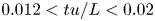 $0.012< tu/L<0.02$, vertical velocity components decrease while remaining positive. This means that elastic plates are still moving upwards (recall that the peak pressure of elastic cases emerges when the plate reaches its maximum deflection; see figures 3a,b,i,d). Over the same period, vertical velocity components under the elastic plates become greater than those of the rigid plate (see insets of figures 5a–c). This demonstrates that, as compared to a rigid case, the fluid moving towards the elastic plates had lost momentum over
  $tu/L < 0.012$. Thus before the peak velocity (
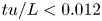 $tu/L<0.012$), fluid momentum was transferred to the solid body.

Figure 5. Time history curves of vertical velocity components at the different points locating on a line with  $z=-0.005L$. Plots (a–c) illustrate the results recorded at
  $x=0$ ,
  $x=L/4$ and
  $x=3L/8$. A close-up view of the time history of each vertical velocity component over
  $0.012 < tu/L <0.019$ is shown in the insets.
Patterns of the vertical (figures 6a–c) and horizontal (figures 6d–f) velocity components of the fluid along  $z=-0.005L$ are shown in figure 6. At the edge of all three plates (
 $x = 0.5L$), the vertical velocity component is maximised after the impact (
 $tu/L>0.02$). This can be explained by the water detachment occurring at the edge of the plate. At
  $tu/L = 0.017$, the vertical velocity component shows some oscillations along
  $z=-0.005L$ at
  $x \approx 0.492 L$. This is perhaps a local artificial effect. The vertical velocity gradient is seen to change from a positive value to a very large negative value from one finite cell to another. This does not seem to be realistic, and is mostly a singularity that is likely to occur due to aspect ratios of the cells under the plate that are greater than 1.0. Note that this behaviour is observed over only a limited length (as compared to the length of the body) and emerges over a very short period of time. Thus it may not have significant effect on the peak pressure, peak deflection and stresses arising in the solid body.

Figure 6. Curves showing distribution of (a–c) vertical and (d–f) horizontal velocity components along a horizontal line located at  $z=-0.005L$. (a,d) Results corresponding to the rigid plate; (b,e) results corresponding to the elastic plate with fixed ends; (c, f) results corresponding to the elastic plate with free ends.
For the rigid plate case (figure 6a), vertical velocity converges to zero over  $0 \leq x \leq 0.45$ (see dash-dotted curves in figure 6a). When elasticity effects are considered, a local minimum is seen to emerge at
  $x \approx 0.04L$ after the water impinges upon the elastic plate (dashed and dash-dotted curves in figure 6c). This is due mainly to the elastic motions of the plate affecting the fluid motion near the plate edges.
Along the  $z=-0.005L$ line, the horizontal velocity component is nearly zero under the mid-point and increases along the plate length. This pattern matches with our physical understanding, i.e. the fluid particles tend to move towards the plate edges where water detachment happens. At the very early stage of the impact (
 $tu/L = 0.017$), the maximum value of
  $v_{x}$ corresponding to a rigid plate and an elastic plate with fixed ends (which emerges at
  $x \approx 0.5L$) is observed to be much greater than values at other instants.
The  $v_{x}$ values under the rigid and elastic plates with fixed ends decrease over time. For the plate with free ends,
  $v_{x}$ along
  $0 < x < 0.35L$ is seen to decrease over time. However, over
  $0.35L < x < 0.5L$, this velocity component may either increase or decrease over time. This is because the ends of the plate are free and may exhibit large motions depending on the temporal displacement rate near the plate edges.
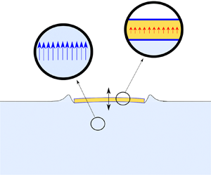
Snapshots of fluid motion around an elastic plate entering water are illustrated in figure 7. At  $tu/L = 0.0175$ (i.e. the time instant that corresponds to an instant before pressure peaks), the pressure under the edges of the elastic plate is larger as compared to
 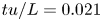 $tu/L = 0.021$ (i.e. the time instant that corresponds to an instant after pressure peaks). This signifies that the pressure under the plate edges significantly decreases after impact. At
  $tu/L = 0.0175$, the velocity magnitude under the plate edges is lower than that observed at
  $tu/L = 0.021$. This confirms that a larger amount of the energy is transferred towards the edge of the plate just after the pressure peaks.

Figure 7. Snapshots showing the fluid motion around an elastic plate entering water. The plate thickness is not to scale.
3.2. Momentum exchange
In this subsection, the exchange of momentum between fluid and solid is studied. Assuming that the solid momentum is caused by the vertical velocity, the sectional momentum (denoted by  $m(x,t)$) along the solid body is calculated as
 \begin{equation} m(x, t)=\int_{0}^{h} \rho_{s}\,v_{y}(x,t) \,{{\rm d}y} . \end{equation}
The momentum of the whole solid body is
 \begin{equation} \mathcal{M}_{s}(t)=\int_{{-}L/2}^{L/2} m(x, t) \,{{\rm d}\kern0.06em x}. \end{equation}
Solid momentum is normalised using the fluid (water) momentum of a control volume displacing an area equivalent to that of the solid body as
 \begin{equation} \mathcal{M}_{in}=\rho_w Lh u. \end{equation}
Figures 8(c,d) display the pattern of the sectional momentum distribution along the solid body at three different instants: right after the impact, when the plate flexes upwards, and when it flexes downwards. The sectional momentum varies locally, and the patterns of momentum distribution along the plate related to plates with different boundary conditions are different, though they are very similar to those of the deflection rates, which were presented in figures 4(n,o). Wherever the displacement is set to be zero, sectional momentum is zero (points with  $d(t)=0$ in figures 8a,b).

Figure 8. (c,d) Sectional momentum along the elastic plates, and (e,f) time history of the momentum of these plates (a,b).
The time history of the momentum of the solid body is plotted in figure 8(e) (plate with two fixed ends) and figure 8( f) (plate with two free ends). A maximum value of the momentum emerges right after the impact (i.e. when water reaches the solid body). The wet condition of the plate is marked with a red background. The first crest of momentum is generated by the fluid force (the impact force). This value of the crest is denoted with  $\mathcal {M}_{E}^{*}$. This crest emerges when the vertical speed at all points is maximised. Afterwards, the momentum varies harmonically. This again confirms that the deflection of the solid body impacted by the water is composed of an exponential and a harmonic response. Note that momentum is found using the deflection rate, i.e. time derivative of the deflection. The solid momentum decays over time. This is because the motions decay over time and thus the resulting momentum harmonically varying over time is gradually given back to the fluid. Note also that whenever the solid momentum is zero, the displacement at all points has reached a crest. If we assume that no fluid and solid damping is activated before solid momentum reaches the first crest, then solid momentum can be formulated as
 \begin{equation} \mathcal{M}_{s} \approx \mathcal{M}_{E}^{*} \sin \left(\frac{2{\rm \pi}}{T}\,(t-t_{w}) \right), \quad t_{w}< t< t_{w} + T/4, \end{equation}
where  $T$ is the natural period of the plate corresponding to the lowest natural frequency, and
  $t_{w}$ is the wetting time. The momentum in the solid body fluctuates before wetting begins. This happens because the plate tends to find its equilibrium before the impact occurs. The problem was run for different initial water levels, which lead to different wetting times. It has been observed that different initial water levels do not affect the momentum arising in the solid body and the resulting peak pressure. In addition, the first crest of the momentum in the solid body is lower as compared to the absolute value of first recorded trough. This happens as the plate has not reached its maximum deflection, and strain energy has not been fully developed in the solid body, though the kinetic energy has already reached its first crest. When the plate moves downwards, reaching its initial location, momentum reaches its first trough. In this condition, the strain energy is turned into kinetic energy. Thus the absolute value of first trough of momentum is larger than the first crest.
Figure 9 displays the time history of the power of the elastic body. Power (denoted  $\dot {W}$, where
  $W$ represents work) is found as
 \begin{equation} \dot{W} = \int_{{-}L/2}^{L/2} p v_y \,{\rm d} \boldsymbol{\varGamma} ,\quad \text{on }\{x, y\} \in \boldsymbol{\varGamma}_{FS}. \end{equation}
This can be normalised by using the energy flux passing through a surface with length  $L$, given by
 \begin{equation} P = 0.5 \rho_w L u^{3} . \end{equation}
Work is found by integrating power over time:
 \begin{equation} W(t) = \int_{0}^{t} \dot{W} \,{\rm d} \tau. \end{equation}
We normalise  $W$ using kinematic energy of fluid (
 $KE$) displacing for a volume equal to that of the solid body, given by
 \begin{equation} KE = 0.5 \rho_{w} hL u^{2}. \end{equation}
Figure 9. Time history curves of (a) the time rate of work and (b) work done by fluid and elastic plates.
Power reaches a positive peak, followed by a negative peak (figure 9a). The positive peak emerges when the momentum has reached its first crest, and the negative peak emerges when the first trough of the momentum emerges. The peak positive and peak negative of the first cycle are seen to be relatively close, though the first half-cycle lasts for a relatively longer time. This leads to a peak in the time history of work, which abruptly decreases, converging to a non-zero value. The power related to the plate with fixed ends is relatively greater than that of the plate with elastic ends. This reflects that a larger amount of work is required to bend a plate with fixed ends, as compared to a plate with free ends. Interestingly, the first crests of power and work are much larger than the following crests. This again demonstrates that the dynamic response of the solid body is composed of an exponential term corresponding to the impact load and harmonic response corresponding to natural frequency, as is shown in Appendix E.
3.3. Effects of momentum exchange on hydroelastic response
The problem has been solved for different values of Young's modulus and thickness, as summarised in table 2. Five different impact velocities,  $0.112\,\textrm {m}\,\textrm {s}^{-1}$,
  $0.235\,\textrm {m}\,\textrm {s}^{-1}$,
  $0.47\,\textrm {m}\,\textrm {s}^{-1}$,
  $0.70\,\textrm {m}\,\textrm {s}^{-1}$ and
  $0.95\,\textrm {m}\,\textrm {s}^{-1}$, are considered. The momentum exchange, denoted
  $\mathcal {M}_{E}^{*}/\mathcal {M}_{in}$, was evaluated, and data were plotted as a function of non-dimensional impact speed, normalised as
 \begin{equation} \mathcal{U}=u \sqrt{\rho_s/E}, \end{equation}
where  $\mathcal {U}$ incorporates Young's modulus of the elastic body and its density, which helps us to study the effects of elasticity and impact velocity on any acquired parameter. Since
  $\mathcal {U}$ is the square root of the Cauchy number, it quantifies the importance of consideration of elastic forces. Note that the density of the body is set to be
  $2.6 \rho _w$ in all simulations.
Table 2. Cases run in the present research, and markers used to plot the data.

In some previous studies (e.g. Stenius, Rosén & Kuttenkeuler Reference Stenius, Rosén and Kuttenkeuler2007; Datta & Siddiqui Reference Datta and Siddiqui2016; Feng et al. Reference Feng, Zhang, Wan, Jiang, Sun and Zong2021), different parameters are normalised using the values found for static tests (e.g. deflection), and impact speed is normalised using the loading period, which can be done only for a wedge section, not a flat plate. Such an approach for normalisation, while interesting, cannot be applied here. This is because we do not aim to study the dynamic effects (the ratio of results of a dynamic case to a static case) or a wedge water entry.
We plot  $\mathcal {M}_{E}^{*}/\mathcal {M}_{in}$ as a function of
  $\mathcal {U}$ with an aim to identifying the link between the momentum exchange and the impact speed (see figure 10). Here,
  $\mathcal {M}_{E}^{*}/\mathcal {M}_{in}$ is seen to increase linearly as a function of
  $\mathcal {U}$. This matches with our expectations. Imagine that a hydrodynamic force (
 $F(t) \propto u^2$) causes the rise of momentum in a solid medium. This can be formulated as
 \begin{equation} \mathcal{M}_{E}^{*} \approx \int_{t_w}^{t_w+T/4} F(t) \,{\rm d}t. \end{equation}
Thus  $\mathcal {M}_{E}^{*}$ would be proportional to
  $u^2$. It was also observed that pressure acting on a plate shows harmonic behaviour (see figures 3a–c). This means that before the fluid momentum reaches its peak value (i.e.
  $t< T/4$), the force will be proportional to
  $T$. Hence
  $\mathcal {M}_{E}^{*}$ is expected to be proportional to
  $T$, which in turn is proportional to
  $E^{-0.5}$ (Stenius et al. Reference Stenius, Rosén and Kuttenkeuler2007). Thus
  $\mathcal {M}_{E}^{*}/\mathcal {M}_{in}$ is expected to be proportional to
  $\mathcal {U}$ (i.e.
  $uE^{-0.5}$), and
  $\mathcal {M}_{E}^{*}/\mathcal {M}_{in}$ is formulated as
 \begin{equation} \mathcal{M}_{E}^{*}/\mathcal{M}_{in} \approx \mathcal{A} \mathcal{U}, \end{equation}
where  $\mathcal {A}$ is a constant value that depends on the thickness of the plate and its boundary conditions (see table 3). For a thinner plate,
  $\mathcal {M}_{E}^{*}/\mathcal {M}_{in}$ increases at a greater rate, and
  $\mathcal {A}$ is slightly larger. A thinner plate is less rigid, thus it flexes more easily. Its solid momentum is larger as compared to a body with a greater rigidity. The results corresponding to the plate with two free ends are seen to be relatively smaller as compared to those of plates with two fixed ends (compare figures 10a,b). From a physical point of view, the free–free boundary conditions may explain such behaviour. The value of
  $\mathcal {M}_{E}^{*}/\mathcal {M}_{in}$ depends on the first bending of the plate. For a plate with two fixed ends, the plate bends in the middle, and at both ends, the plate points downwards (figure 4k). As such, the fluid motion tends towards the vertical direction and downwards (figure 4n). This increases the exchange of the momentum between the fluid and solid. On the other hand, for a plate with two free ends, the ends bend upwards (figures 4j,m). Consequently, the exchange of momentum between fluid and solid is reduced.

Figure 10. The first crest of momentum, arising in plates with (a) fixed and (b) free ends, just after impact, as a function of the dimensionless impact speed.
Table 3. Constant coefficients found using curve fitting.

Assuming that  $\mathcal {M}_{E}^{*}/\mathcal {M}_{in}$ decreases exponentially (which can be seen in figures 8(e,f), see the dashed grey curves), the temporal decay of crests
  $\mathcal {M}_{E}^{*}/\mathcal {M}_{in}$ can be represented as
 \begin{equation} \psi(t+nT) \approx \psi_2\,{\rm e}^ {- \alpha (t+nT)}, \quad n \in \mathbb{N} -\{1\}. \end{equation}
Here,  $\alpha$ is the temporal decay rate, and
  $\psi$ is every recorded crest. The value of
  $\alpha$ is normalised using
 \begin{equation} \alpha^{*} = \alpha h / u. \end{equation}
This  $\alpha ^{*}$, the decay rate of the momentum in the solid body, is plotted versus
  $\mathcal {M}_{E}^{*}/\mathcal {M}_{in}$ in figure 11;
  $\alpha ^{*}$ decreases as
  $\mathcal {M}_{E}^{*}/\mathcal {M}_{in}$ increases. Note that
  $\alpha$ corresponding to different thicknesses is seen to be relatively constant over the range of different
  $\mathcal {M}_{E}^{*}/\mathcal {M}_{in}>0.15$. This means that damping is likely to be caused by the free surface deformation near the plate (which depends on the geometry) and depends mostly on the dimensions of the plate and its boundary conditions, not viscosity. For lower values of
  $\mathcal {M}_{E}^{*}/\mathcal {M}_{in}$, the impact process may not be fully developed, thus the damping mechanism may also be caused by some other mechanisms (break of free surface). To match it with our expectation,
  $\alpha ^{*}$, is formulated as
 \begin{equation} \alpha^{*} \approx \mathcal{B} (\mathcal{M}_{E}^{*}/\mathcal{M}_{in})^{{-}1}. \end{equation}
Here,  $\mathcal {B}$ values are sensitive to
  $h/L$ and boundary conditions, which are presented in table 3. The fitted curves are plotted in figures 11(a,b). Parametrisation is carried out by excluding the data related to low values of
  $\mathcal {M}_{E}^{*}/\mathcal {M}_{in}$.

Figure 11. Decay rates of the momentum of the plates with (a) fixed and (b) free ends.
The peak pressures acting on elastic plates are normalised on the basis of the rigid case. This ratio is called the relative pressure, and is plotted versus  $\mathcal {M}_{E}^{*}/\mathcal {M}_{in}$ in figure 12. Relative pressure reduces linearly as a function of
  $\mathcal {M}_{E}^{*}/\mathcal {M}_{in}$. This suggests that exchange of momentum is linked to pressure reduction. The values of
  $p_f/p_r$ related to different thicknesses and Young's modulus are seen to follow a linear line when they are plotted as a function of
  $\mathcal {M}_{E}^{*}/\mathcal {M}_{in}$ (figures 12a,b). For both boundary conditions, the relative values of maximum pressure decrease linearly with the increase of
  $\mathcal {M}_{E}^{*}/\mathcal {M}_{in}$.

Figure 12. Values of relative pressure of plates with (a) fixed and (b) free ends.
To relate the impact pressure acting on the elastic body to that of the rigid body, we assume that the proportion of momentum that is transferred to the solid body reduces the peak pressure. We start with the rigid body. We assume that a mass of water with initial momentum  ${M}_{0} = C_{0}\mathcal {M}_{in}$ flows towards the plate, and its vertical momentum becomes zero in a very short time
  $\Delta t$. Using the von Kármán water entry theory (von Kármán Reference von Kármán1929), the average pressure can be estimated using the momentum variation as
 \begin{equation} \bar{p}_r \approx \frac{C_{0}\mathcal{M}_{in}}{L\,\Delta t}. \end{equation}
The average pressure acting on an elastic plate is caused by a reduced momentum ( $C_{0}\mathcal {M}_{in}-\mathcal {M}_{E}^{*}$), which can be written as
 \begin{equation} \bar{p}_f \approx \frac{C_{0}\mathcal{M}_{in}-\mathcal{M}_{E}^{*}}{L\,\Delta t}. \end{equation}
Using (3.16) and (3.17), the relative average pressure acting on an elastic plate can be formulated as
 \begin{equation} \bar{p}_f/\overline{p}_r \approx 1 - (\mathcal{M}_{E}^{*}/C_{0}\mathcal{M}_{in}). \end{equation}
Equation (3.18) can be viewed as an extension of von Kármán water entry theory for an elastic plate, and is derived by assuming that  $\Delta t$ values related to both rigid and flexible cases are equal, and some physical aspect may have been overlooked. Note that von Kármán (Reference von Kármán1929) formulated the initial momentum using the added mass of the object entering the water. Equation (3.18) is derived to predict the average pressure. It is rewritten to predict peak pressure by introducing a new non-dimensional coefficient (
 $\mathcal {C}$) as
 \begin{equation} p_f/p_r \approx 1 - \mathcal{C} (\mathcal{M}_{E}^{*}/\mathcal{M}_{in}). \end{equation}
The best fitted values of  $\mathcal {C}$ are shown in table 3. However, the data related to the most flexible case are not considered as they may lead to nonlinear effects, which cannot be estimated using a linear function.
Interestingly,  $\mathcal {C}$ values found for both plates – either the one with two fixed ends or the one with two free ends – are very close. To sum up, the relative impact pressure can be a function of momentum exchange, regardless of the boundary conditions set for a plate or the thickness of the structure. This matches well with the general hypothesis of the present research namely ‘the transfer of momentum from the fluid to solid, caused by the flexible motions, is the main mechanism that reduces the impact pressure’. From a practical perspective, this means that the hydroelastic response of a structure impacted by water can be predicted using the data found through the rigid simulations (see figure 12). The peak pressure is a local effect, and the momentum exchange is a global term. The paper attempts to simply suggest the concept of a method and not propose a conclusive unified solution. Therefore the relationship between a global term and a local term is formalised on the basis of peak pressure.
Through tracking the time history of the deflection of the plate, the maximum deformation during each water entry process is found. Dimensionless maximum deformation values versus the values of  $\mathcal {M}_{E}^{*}/\mathcal {M}_{in}$ are plotted in figures 13(a,b). Maximum deformation grows with the increase in (
 $\mathcal {M}_{E}^{*}/\mathcal {M}_{in}$). The data corresponding to the plates with different Young's modulus values and thicknesses (figures 13a,b) fit well. This supports the hypotheses that the hydroelastic responses of a body entering water can be formulated using simple equations as a function of momentum exchange.

Figure 13. Maximum values of non-dimensional deformation of plates with (a) fixed and (b) free ends.
Maximum deflection of an Euler–Bernoulli beam is proportional to force, and inversely proportional to Young's modulus. Thus
 \begin{equation} d_{max} \propto \frac{F}{E}. \end{equation}
 Since  $F$ is proportional to
  $u^2$, maximum deformation is expected to be proportional to
  $u^2/E$ (i.e.
  $\mathcal {U}^2$). Accordingly, the dimensionless maximum deformations can be fitted on the basis of the equation
 \begin{equation} d_{max}/ L \approx \mathcal{D} (\mathcal{M}_{E}^{*}/\mathcal{M}_{in})^2, \end{equation}
where  $\mathcal {D}$ is a constant value that depends on the boundary conditions and plate thickness (see table 3). For the plate with two free ends,
  $\mathcal {D}$ values corresponding to
  $h/L=0.05$ and
  $h/L=0.1$ are nearly equal.
The relationship between the maximum value of dimensionless equivalent stress and  $\mathcal {M}_{E}^{*}/\mathcal {M}_{in}$ is analysed. Peaks of the recorded equivalent stress at every point are found, and the maximum peak is set to be the maximum dimensionless equivalent stress. Data are plotted in figure 14. The maximum dimensionless equivalent stress is constant up to a specific value of
  $\mathcal {M}_{E}^{*}/\mathcal {M}_{in}$, then it decreases under the increase of
  $\mathcal {M}_{E}^{*}/\mathcal {M}_{in}$. This constant value is called the maximum potential stress emerging in an elastic body impacted by the water. The
  $\mathcal {M}_{E}^{*}/\mathcal {M}_{in}$ value that marks the limit at which the divergence of the stress from the maximum potential stress occurs is termed the critical momentum exchange. In general, the data plotted in figure 14 signify that the maximum potential stress on a plate impacted by the water may not be acquired when the momentum exchange gets larger than the critical limit. This happens when the impact speed gets higher and the water entry problem occurs in a shorter time, i.e. when stresses may not be fully developed.

Figure 14. Maximum dimensionless equivalent stress of plates with (a) fixed and (b) free ends.
The relationship between the maximum dimensionless stress and the fluid–solid momentum exchange is
 \begin{equation} \sigma_{max} / (0.5 \rho_s u^2) \approx \begin{cases} \mathcal{E}, & \mathcal{M}_{E}^{*}/\mathcal{M}_{in} \leq \mathcal{F}, \\ \mathcal{E} - \mathcal{G} ( \mathcal{M}_{E}^{*}/\mathcal{M}_{in} -\mathcal{F} ), & \mathcal{M}_{E}^{*}/\mathcal{M}_{in} > \mathcal{F}. \end{cases} \end{equation}
Here,  $\mathcal {E}$ is a constant value referring to the maximum potential stress that can be developed in the solid body,
  $\mathcal {F}$ is the critical value of fluid–solid momentum exchange, and
  $\mathcal {G}$ is a constant value that reflects the slope of the deviation of maximum stress from the maximum potential stress. Values of these coefficients are given in table 3. At present, no theoretical background for (3.22) can be established. Yet the linear decrease of the stress as a function of
  $\mathcal {M}_{E}^{*}/\mathcal {M}_{in}$ explains the linear decrease of the peak pressure versus
  $\mathcal {M}_{E}^{*}/\mathcal {M}_{in}$ plots (see figure 12).
The maximum stresses ( $\mathcal {E}$) arising in a thin plate are greater as this solid body has a lower second moment of area. Boundary conditions may also influence the results; i.e. for plates with two free ends, the maximum stresses are slightly smaller as compared to those of plates with fixed ends. Only the displacement is set to be zero at the middle point, thus the maximum equivalent stresses are lower.
It should be noted that OpenFOAM code used for simulation of the present problem does not use model analysis. Instead, the solid dynamic response is found through solving the conservation of momentum in a solid medium. For an elastic flat plate entering water, the pressure reaches its peak value in a very short period of time. The maximum deflection occurs during the free vibration phase, and the lowest eigenvector dominates the response (Faltinsen Reference Faltinsen2000). In addition, the first crest of momentum in the solid happens before the peak pressure and deflection emerge. This means that the response of the plate incorporates an exponential term and a harmonic one. The latter corresponds to the lowest natural frequency. Hence the role of higher-order structural deformations is not considered that important (Pochyly, Malenovsky & Pohanka Reference Pochyly, Malenovsky and Pohanka2013; Yan et al. Reference Yan, Mikkola, Kujala and Hirdaris2022a). Contrary to this, for wedge sections entering water, the loading period is longer as compared to the case of a flat plate (Wang & Guedes Soares Reference Wang and Guedes Soares2018; Yan et al. Reference Yan, Mikkola, Kujala and Hirdaris2022a). Therefore, future research could focus more on such investigations.
4. Conclusions
The pressures and forces arising during the water entry of an object can be reduced when the body is flexible as stresses and deformations emerge. From an engineering point view, it is very important to provide closed-form equations that calculate the pressure and hydroelastic responses of a flexible body impinging. With the latter in mind, this paper aimed to present a new methodology for the analysis of hydroelastic responses of a flat plate entering water using the momentum that is transferred to the solid body just after impact. The research study assumes that the pressure arising at the water entry can be extracted from rigid body simulations using the potential momentum exchange facilitated by fluid and solid interactions. Another hypothesis is that the potential momentum exchange can be used to calculate the deformations and stresses during water entry.
The problem was solved for a plate with fixed and free ends. This assisted with validating the main hypothesis of the present study for the simplest case. The plate with free ends was found to show a fluttering motion, leading to larger displacement. However, the maximum equivalent stress acquired during the water entry was observed to be lower. The time history of the momentum of the solid body undergoes a harmonic idealisation, though it was found to decay exponentially over time. Although no solid-based dissipative mechanism was set to constrain the simulation, the decay rate of the momentum was seen to be a function of the peak value of the momentum arising in the solid body.
The relative pressure – namely, the ratio of maximum pressure of elastic plate to that of the rigid plate – was calculated, and was demonstrated to be a function of the amount of the momentum transferred to the solid body, regardless of the thickness and elastic modulus of the body. The latter supports the main hypothesis that maximum pressure acting on an elastic structure can be formulated as a function of momentum exchange using the maximum value of a rigid plate.
It was shown that the maximum dimensionless deformation of flat plates entering water can be formulated as a function of the momentum exchange. The same approach was used to investigate the relationship between the maximum dimensionless equivalent stress acquired during the impact process. This stress was seen to be constant over a range of momentum. The momentum at which the change in the dimensionless equivalent stress emerges was called the critical momentum. It was shown that as the momentum exchange becomes greater than the critical value of the dimensionless equivalent, stress decreases linearly. This helped us to formulate maximum equivalent stress as a function of momentum exchange. The formulation presented for dimensionless deformation and stress provided evidence that the hypothesis of the present research is valid for our simulations, and these two dependencies can be formulated as a function of momentum exchange.
Overall, the momentum that is transferred from water to an elastic solid body entering water can be estimated using a simple linear equation, the value of which can then be used for the evaluation of relative pressure, the maximum deformation and equivalent stress. Thus a rigid body simulation of the problem would be enough to reach the data of an elastic water entry. This may be significant as economic yet accurate engineering solutions may lead to much needed practical solution of FSI problems for use in the design of ships and offshore structures. The results presented are limited to the case of an elastic flat plate. Further investigations regarding the influence of momentum exchange mechanisms and their relationships with responses of wedge and ship bow sections will be a significant part of future research efforts. Such an approach may help us to improve understanding of physics and explore the usefulness of the method in relation to traditional hydroelasticity approaches (Hirdaris & Temarel Reference Hirdaris and Temarel2009; Yan et al. Reference Yan, Mikkola, Kujala and Hirdaris2022a), and validate the solution.
The study presented in this paper can be extended further to other marine structures and or bodies found naturally in the ocean (e.g. marine vegetation). The fluid motion can be assumed to have steady or cyclic motions, the latter of which represents a wave-induced motions scenario. Justification of the latter requires running further numerical simulations. Also, modified versions of formulations should be presented for other bodies as their loading period during the water entry process is much longer compared to that of horizontal flat plates. In future, equations presented for momentum can be changed to consider local momentum, which may help us to formulate equations with less restriction. Finally, it should be noted that the present model neglects compressible fluid motion, which can be incorporated in the future.
Acknowledgements
The authors are very thankful to anonymous reviewers of this paper who provided constructive comments that helped them to enhance the quality of the paper.
Funding
The authors acknowledge financial support by Aalto University and the Finnish Maritime Foundation (Merenkulun säätiö).
Declaration of interests
The authors declare that they have no known competing financial interests or personal relationships that could have appeared to influence the work reported in this paper.
Appendix A. Mesh convergence study
A mesh sensitivity study is performed as explained in the main text of the paper. The aim is to find the optimised mesh that can be used to simulate the problem.
Four different meshes with different resolutions are generated, and runs using OpenFOAM are performed to reproduce the air–water flow around a plate impacted by the water. Meshes are named coarse, medium, fine and finest. In the fluid domain, the cell size of the coarse mesh under the wall of the plate is  $0.016 L \times 0.005 L$, though that of finest mesh is
  $0.008 L \times 0.0016 L$. The cell sizes of the medium and fine fluid meshes under the plate are respectively
  $0.01 L \times 0.003 L$ and
  $0.005 L \times 0.0018 L$. In the solid domain, the cell size of the coarse mesh is
  $0.02 L \times 0.005 L$, while that of the finest mesh is
  $0.01 L \times 0.0018 L$. The cell sizes of the medium and fine solid meshes are respectively
  $0.015 L \times 0.003 L$ and
  $0.008 L \times 0.0024 L$. The plate is set to have thickness
  $0.1L$, and the impact speed is prescribed to be
  $0.7\,\textrm {m}\,\textrm {s}^{-1}$. Both ends of the plate are set to be fixed.
The hydroelastic response of the structure is sampled over time, and the related results are presented in figure 15. Figures 15(a,b) display the equivalent stress emerging in the solid body. Figures 15(c,d) show the time history of the vertical motions at two different points. Figures 15(e, f) illustrate the time history of the pressure at two different points. The general behaviour of the time history curves has been explained in the main text of the paper. Time history curves of stresses, deformations and pressure converge with the increase in mesh resolution. The results computed by using fine and finest resolutions practically match.

Figure 15. Mesh study: convergence of the time history curves of (a,b) equivalent stress, (c,d) vertical deformation and (e, f) dimensionless pressure by increasing the mesh resolution. Data are found through performing runs for an impact process with speed  $0.7\,\textrm {m}\,\textrm {s}^{-1}$. The plate was set to have thickness to length ratio
  $0.1$.
Appendix B. Courant number convergence
Simulations are run for different Courant numbers ( $\mathcal {CO}$) to find the suitable one that can be used to run the simulation. A hydroelastic water entry with speed
  $0.49\,\textrm {m}\,\textrm {s}^{-1}$ is run. The plate is clamped at both ends and is
  $0.1L$ thick. Peak values of the pressure and deflection at two different locations,
  $x = 0$ and
  $x = L/4$, are found. Peak values were plotted against
  $\mathcal {CO}$, as shown in figure 16. Maximum pressure rising at
  $x = L/4$ is more sensitive to
  $\mathcal {CO}$, as compared to middle point of the plate. In addition, a larger peak deflection may be captured at
  $x = 0$ and
  $x = L/4$ when
  $\mathcal {CO}$ increases. Peak values of pressure and deflections are seen to converge by decreasing
  $\mathcal {CO}$ from 1 to 0.25. Hence the simulations of the present research are run by setting
  $\mathcal {CO}$ to be 0.25, though they could also be run using greater values (such as 0.4) as the effect of Courant numbers on peak values is not very significant.

Figure 16. Sensitivity of the results to the Courant number. (a,b) Maximum values of pressure recorded at the middle and quarter points, respectively. (c,d) Maximum deflections recorded at the middle and quarter points, respectively.
Appendix C. Domain size study
The size of the domain is set by running the problem for different widths, varying from  $3L$ to
  $7L$. The plate thickness was set to be
  $0.1L$, and the impact speed was enforced to be
  $0.47\,\textrm {m}\,\textrm {s}^{-1}$.
Time traces of pressure and displacement of the middle point found for each domain size are presented in figure 17. As seen, a domain size with width of  ${\geq }5L$ ensures convergence of simulations and cancels out blockage effects. For a domain with a smaller size, dimensionless pressure and displacement of the middle point may be over-predicted. This can be seen in the close-up views of the time histories shown in the insets. It could be attributed to the blockage effect, which can potentially increase the hydrodynamic pressure and resulting solid dynamic response. A fluid domain with a narrower width can slightly increase the natural period of the plate. This is demonstrated in the close-up views, illustrating the hydroelastic response of the plate over
  $0.054 \leq tu/L \leq 0.06$.

Figure 17. Sensitivity of the results to the domain width. Time traces of (a) dimensionless pressure, and (b) displacement of the middle point.
Appendix D. Validation
D.1. Pressure acting on a rigid plate entering water
Results of the present model are compared against those of available experimental data documented in Ma et al. (Reference Ma, Causon, Qian, Mingham, Mai, Greaves and Raby2016). Experiments were performed at two different impact speeds,  $5.5\,\textrm {m}\,\textrm {s}^{-1}$ (block 1) and
  $7\,\textrm {m}\,\textrm {s}^{-1}$ (block 2), for three dimensional plates with total weights
  $32\,\textrm {kg}$ and
  $52\,\textrm {kg}$. Pressures were measured at the middle point of the plate and at four symmetric points with similar distance
  ${\approx } 0.44L$ from the mid-point of the plate.
Peak pressures measured in experiments and those found through simulations are illustrated in figure 18. The rigid body simulations were insensitive to the weight of block, though those of experiments may depend on the weight of block.

Figure 18. Comparisons between experimental peak pressures of a rigid plate entering water and those of the present model. (a,b) Peak pressures recorded at the middle point of the plate. (c,d) Peak pressures recorded at a point distance  ${\approx } 0.44L$ from the middle point. Experimental data are taken from Ma et al. (Reference Ma, Causon, Qian, Mingham, Mai, Greaves and Raby2016).
Numerical values (dashed line) of peak pressure at the middle point are seen to agree with experimental ones (circle markers) recorded through the water entry tests of block 1 (figures 18a,b). For block 2, numerical values of the peak pressures were found to be relatively larger or lower than the experimental values corresponding to pure water entry tests (figures 18a,b). This can be due to the larger inertia forces, and resulting compressible fluid motions, that are not incorporated in the present model. It is recommended that compressible motion of fluid should be considered in future studies.
Ma et al. (Reference Ma, Causon, Qian, Mingham, Mai, Greaves and Raby2016) observed that peak pressure values at four symmetric points are not equal. They hypothesised that strains arising at the water entry would explain such a difference. To visualise their experimental data, boxplots are presented in figures 18(c,d). Central marks denote the median values of peak pressures at those four symmetric points, and whiskers represent the recorded extreme peak pressures observed at four symmetric points. As seen, for the lower impact speed, numerical peak pressures at  $x \approx 0.44L$ (see the dashed lines in figures 18c,d) are either in the range of experimentally recorded pressures or slightly larger than extreme values (figures 18c,d). Greater values may appear because of the difference between the nature of the present model and the real physics. The present model is built to reconstruct the water entry process of a two-dimensional body, though experiments feature a three-dimensional water entry process. The reason for comparing the results of two-dimensional against three-dimensional cases was the lack of experimental data. Overall, the present model is seen to fairly compute the peak pressure of a rigid body entering water.
D.2. Stain arising in steel plate entering water
The present computational model has been employed to reproduce numerically the water entry of a steel plate with density  ${\approx }7800\,\textrm {kg}\,\textrm {m}^{-3}$ and Young's modulus
  ${\approx }210 \times 10^9\,\textrm {Pa}$. Experiments involving free-fall tests are presented by Kvålsvold, Faltinsen & Aarsnes (Reference Kvålsvold, Faltinsen and Aarsnes1995). The elastic solid body was set to fall from different heights to reach various desired impact speeds. The total weight of the rig was
  ${\approx } 500\,\textrm {kg}$. This potentially cancels out the water exit, leading to a water entry process with a constant rigid impact speed.
The strain emerging in the body is calculated as
 \begin{equation} \epsilon (t) = \frac{\partial}{\partial x}d(t) . \end{equation}
 The temporal strain at the middle point has been monitored, and its peak value was found. This was then compared against experimental measurements found in Kvålsvold et al. (Reference Kvålsvold, Faltinsen and Aarsnes1995) (figure 19). The model slightly over-predicts the maximum strain at  $\mathcal {U} \approx 0.11 \times 10^ {-6}$. The model reconstructs the water entry process with a constant heave speed. However, in experiments, the heave speed is seen to decrease slightly just after the impact. The final impact speed of experiments may be slightly different from the desired one. This is a potential source of uncertainty.

Figure 19. Maximum stain at the middle point of a steel plate entering water at different impact speeds. Circle and triangle markers respectively display experimental and numerical data. Experimental data are taken from Kvalsvold & Faltinsen (Reference Kvalsvold and Faltinsen1995).
Appendix E. Dynamic response of a beam exposed to an impact load
Let  $w$ represent the vertical displacement. Assuming linearity, the dynamic motion of a two-dimensional body over a unit length can be formulated based on the Euler–Bernoulli theory as
 \begin{equation} {\mathfrak{m}\,\frac{\partial^{2} w}{\partial{t}^2} + \mathcal{L}\,\frac{\partial^{4} w}{\partial{x}^4} = F(t),} \end{equation}
where  $\mathfrak {m}$ is mass per unit length of the beam, i.e.
  $\mathfrak {m} = \rho _s h$. In addition,
  $\mathcal {L} = Eh^3/12$ is the sectional rigidity of the beam, and
  $F(t)$ is the impact load acting on the structure, which can be formulated as
 \begin{equation} { F(t) = F_{0}\,{\rm e}^{-\gamma t},} \end{equation}
where  $\gamma$ is the decay rate of the impact force, and
  $F_{0}$ is the peak force. The dynamic response can be reformulated as
 \begin{equation} {\frac{\partial^{2} w}{\partial{t}^2} + k^2\,\frac{\partial^{4} w}{\partial{x}^4} = f_{0}\, {\rm e}^{-\gamma t},} \end{equation}
where  $k = \sqrt {L/\mathfrak {m}}$ is the natural frequency, and
  $f_{0} = F_{0} / \mathfrak {m}$. Performing a Laplace transform, the equation governing the beam dynamic can be written as
 \begin{equation} {s^2 \tilde{w} + k^2\,\frac{\partial^{4} \tilde{w}}{\partial{x}^4} = \tilde{f}(s) }, \end{equation}
where  $\tilde {w}$ and
  $\tilde {f}$ are Laplace transforms of
  $w$ and the right-hand side of (E3), which are respectively given by
 \begin{equation} {\tilde{w} (s) = \int_{0}^{\infty} w\,{\rm e}^{{-}st} \,{\rm d}t} \end{equation}
and
 \begin{equation} {\tilde{f}(s) = \frac{f_{0}}{\gamma + s} }. \end{equation}
Thus the solution of the problem can be established as
 \begin{equation} {\tilde{w} = \frac{f_{0}}{2{\rm i}k}\left(\frac{1}{s+\gamma}\,\frac{2\gamma}{\gamma^2+k^2} + \frac{1}{\gamma+{\rm i}k}\,\frac{1}{s-{\rm i}k} + \frac{1}{\gamma-{\rm i}k}\,\frac{1}{s+{\rm i}k} \right) }. \end{equation}
Using an inverse Laplace transform,  $w(t)$ can be written as
 \begin{equation} {w (t) = \frac{f_0}{k} \left( \frac{2\gamma}{\gamma^2+k^2}\,{\rm e}^{-\gamma t} + \frac{2\gamma \cos{kt} - 2k \sin{kt}}{\gamma^2 + k^2 } \right) } . \end{equation}
As seen in (E8), the dynamic response of the beam impacted by water is composed of an exponential response and a harmonic one, which are also observed in time history curves of the momentum and the work found through the numerical simulations.


 Open access